
The New Volcanic Ash Satellite Retrieval VACOS Using MSG/SEVIRI and Artificial Neural Networks: 2. Validation

 , and
, and
Abstract
:
1. Introduction
2. Performance on Simulated Test Data
2.1. Classification
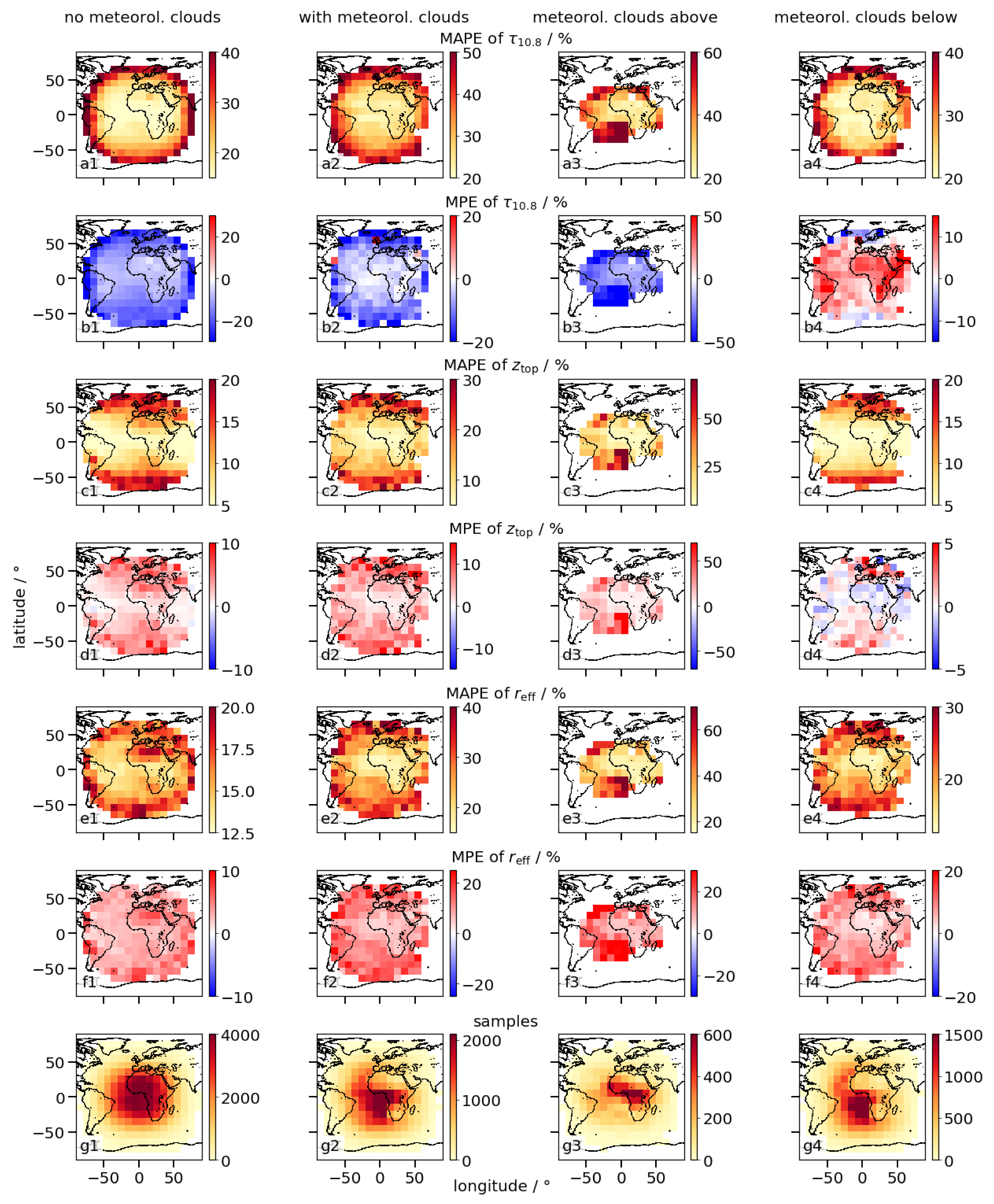
2.2. Dependence on Volcanic Ash Cloud Properties, Meteorological Clouds and Geographic Coordinates
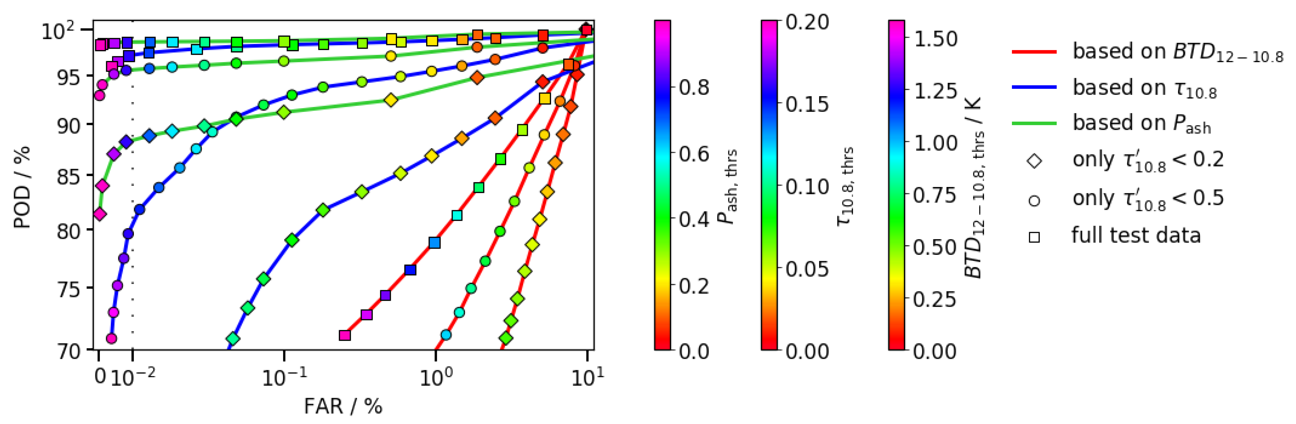
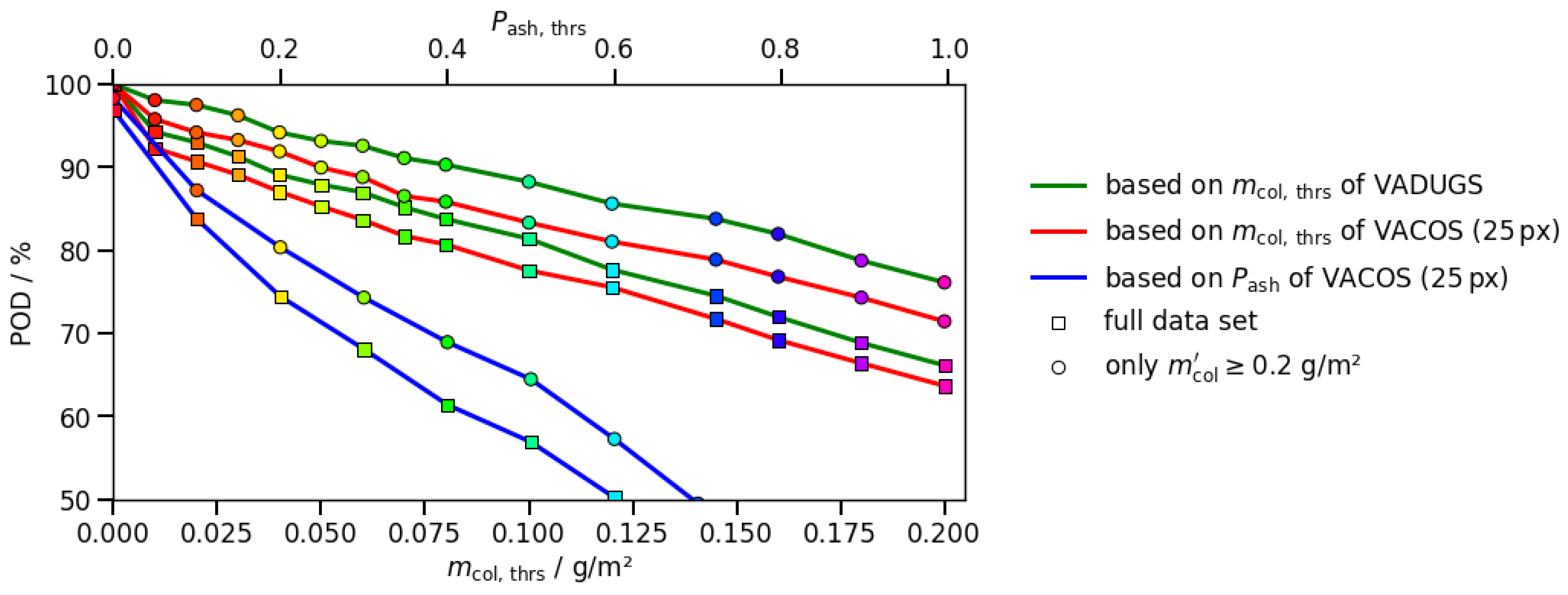
2.3. Detection of Volcanic Ash
3. Sensitivity to Volcanic Ash Cloud Profiles
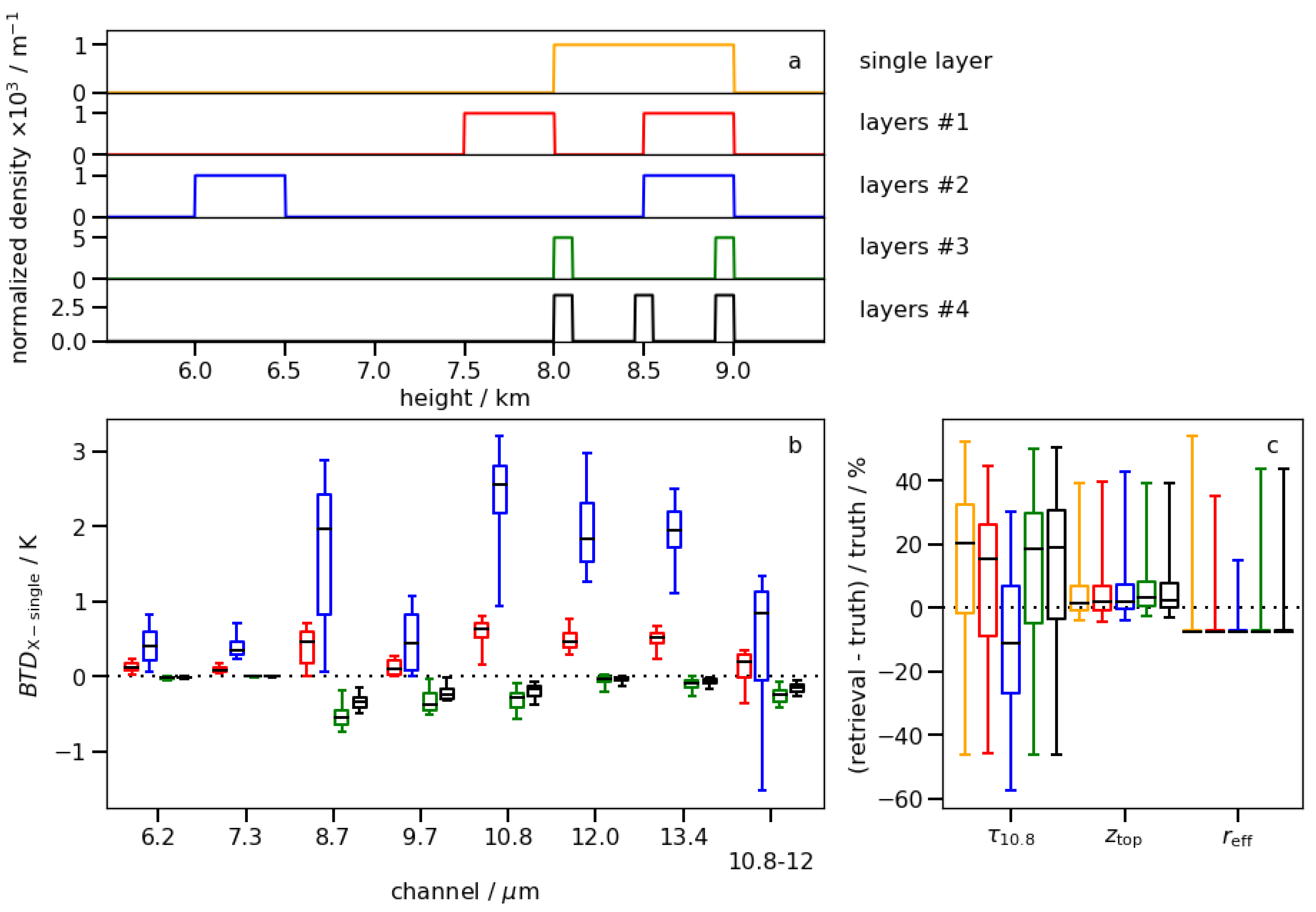
3.1. Multiple Ash Layers
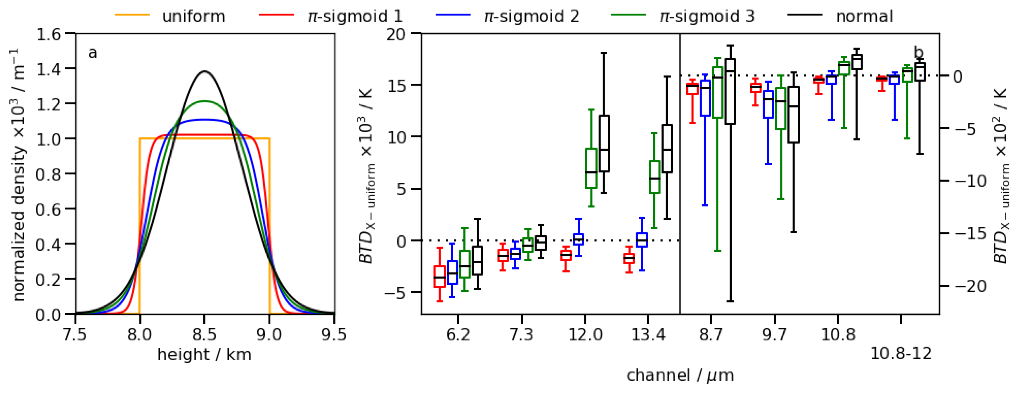
3.2. Non-Homogeneous Ash Profiles
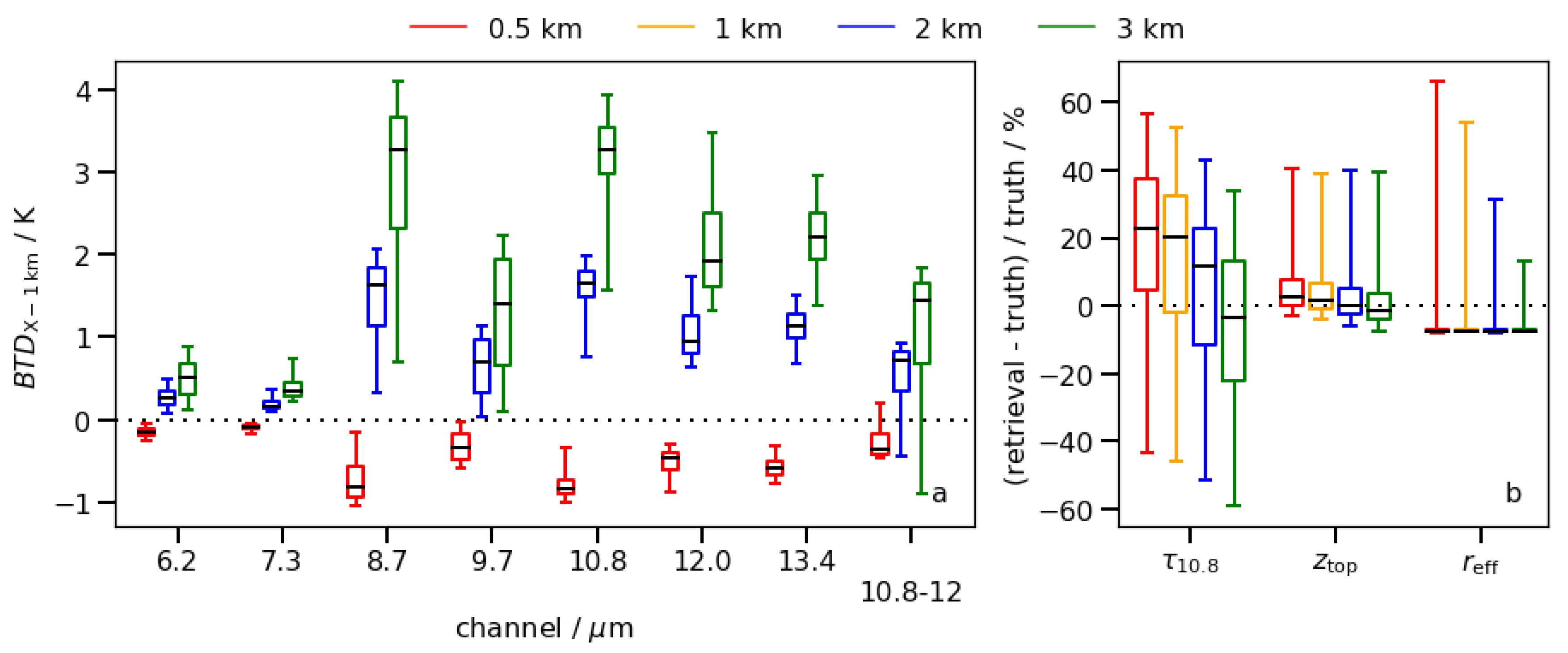
3.3. Geometrical Ash Cloud Thickness
4. Comparisons with Independent Measurements
4.1. Puyehue-Cordón Caulle Eruption (2011)
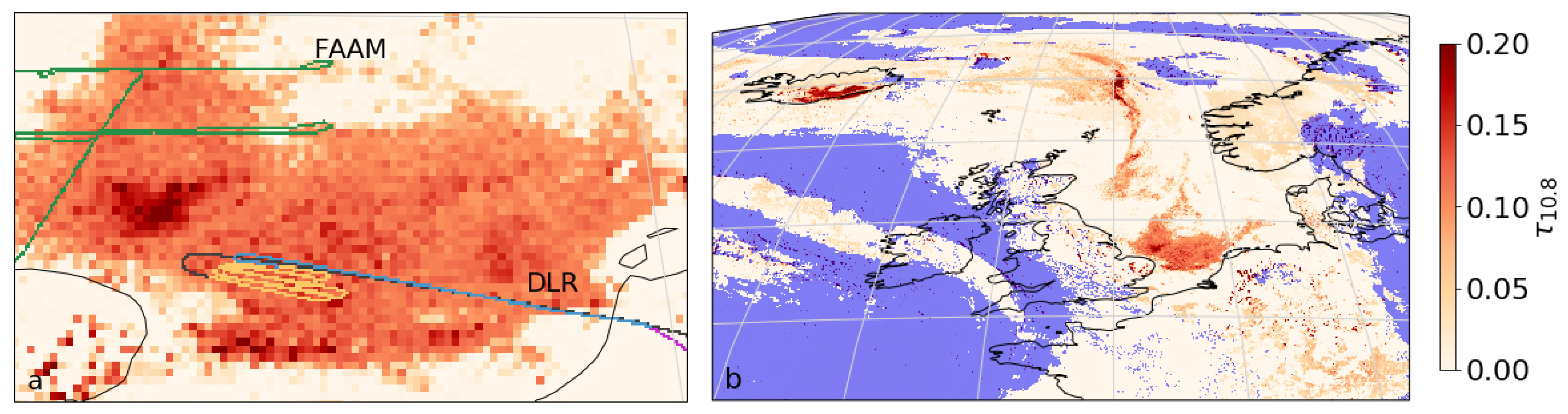
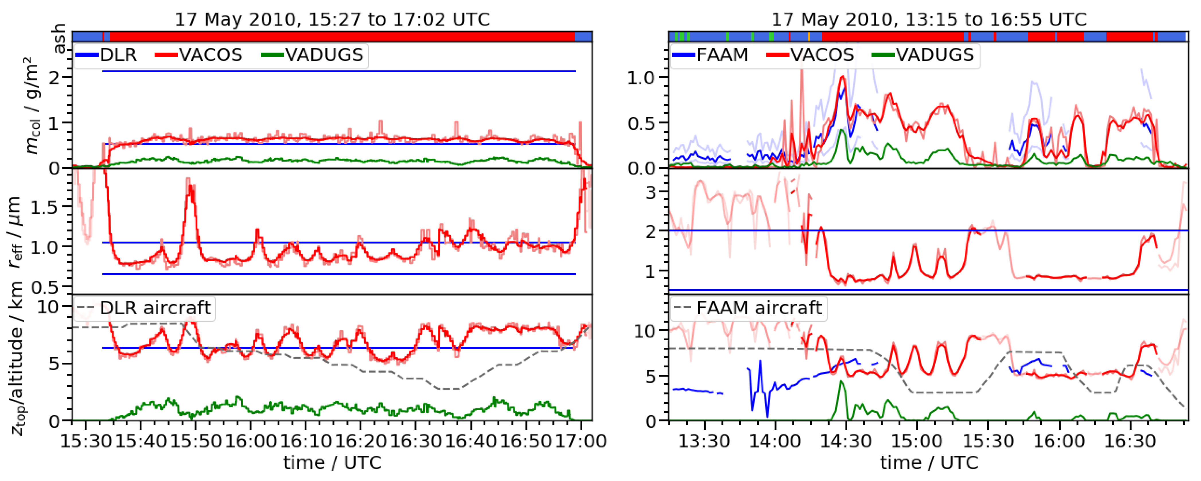
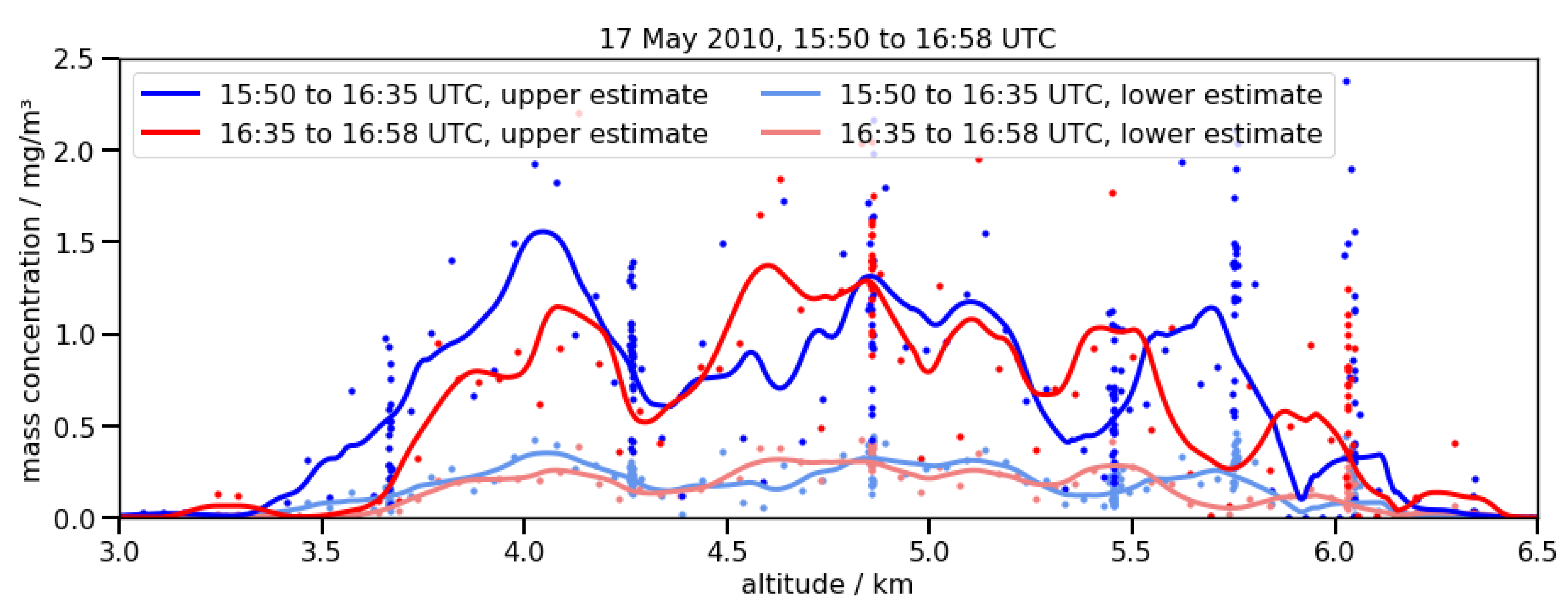
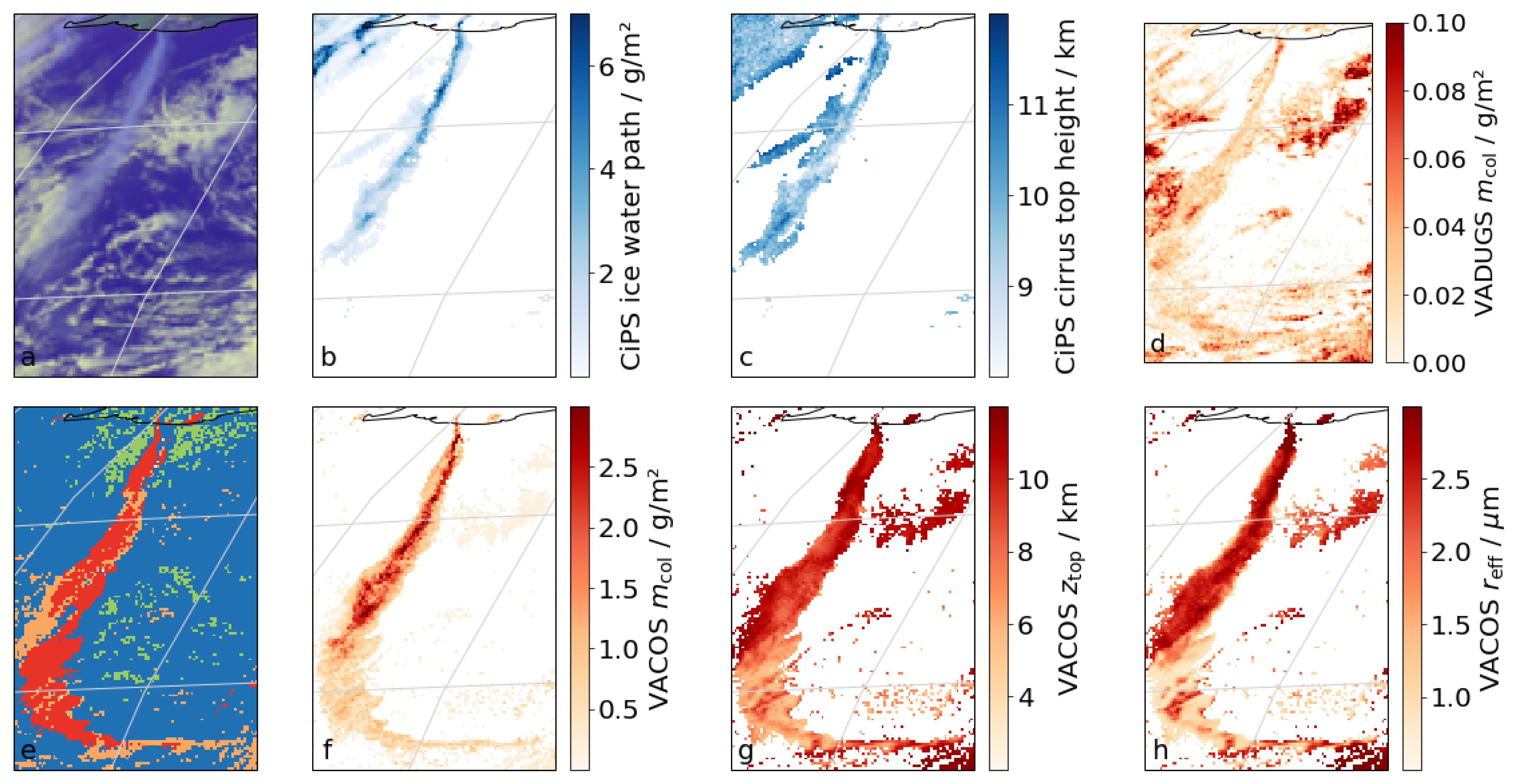
4.2. Eyjafjallajökull Ash Cloud (17 May 2010)
4.3. Eyjafjallajökull Ash Plume at Vent (11 May 2010)
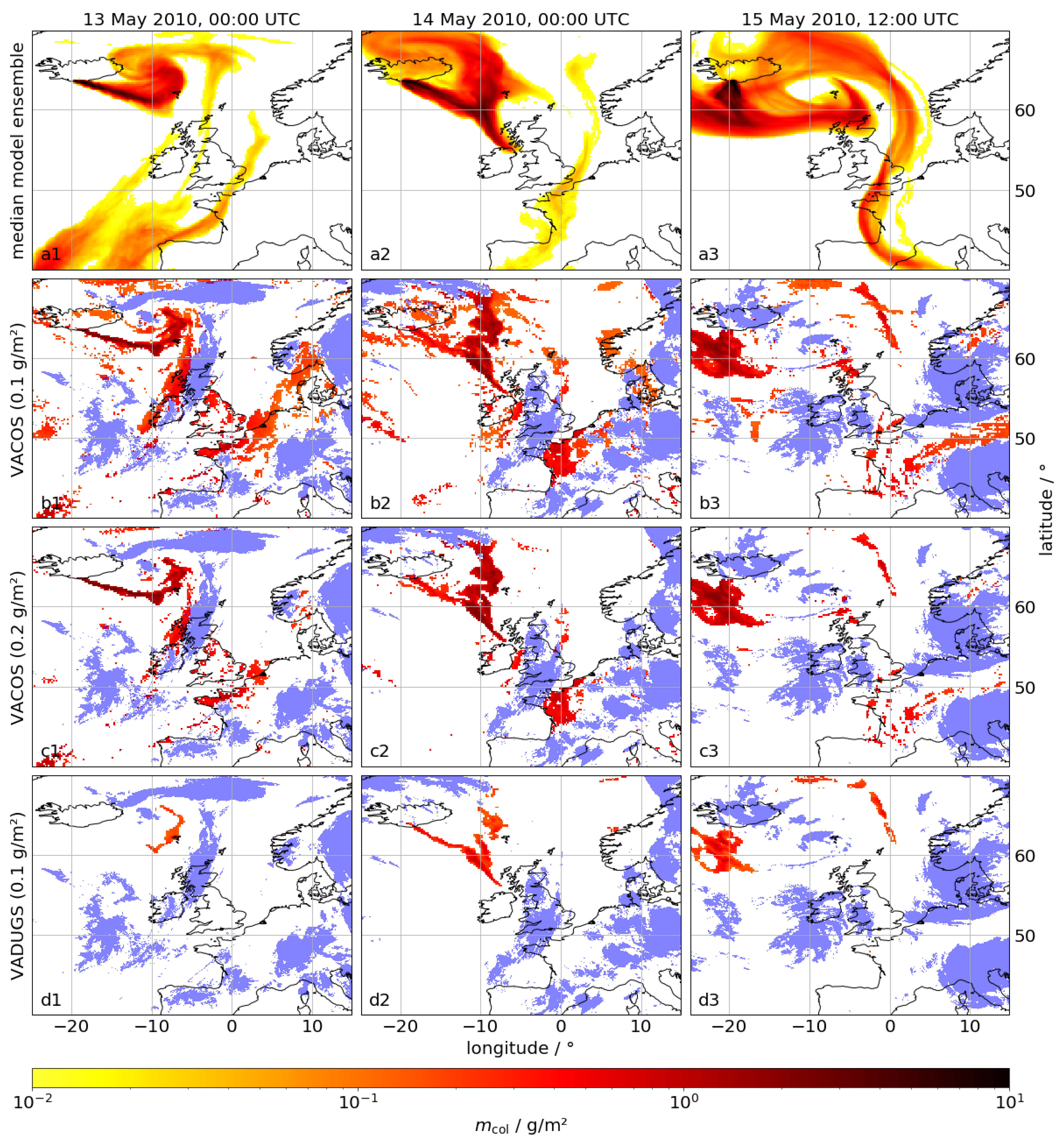
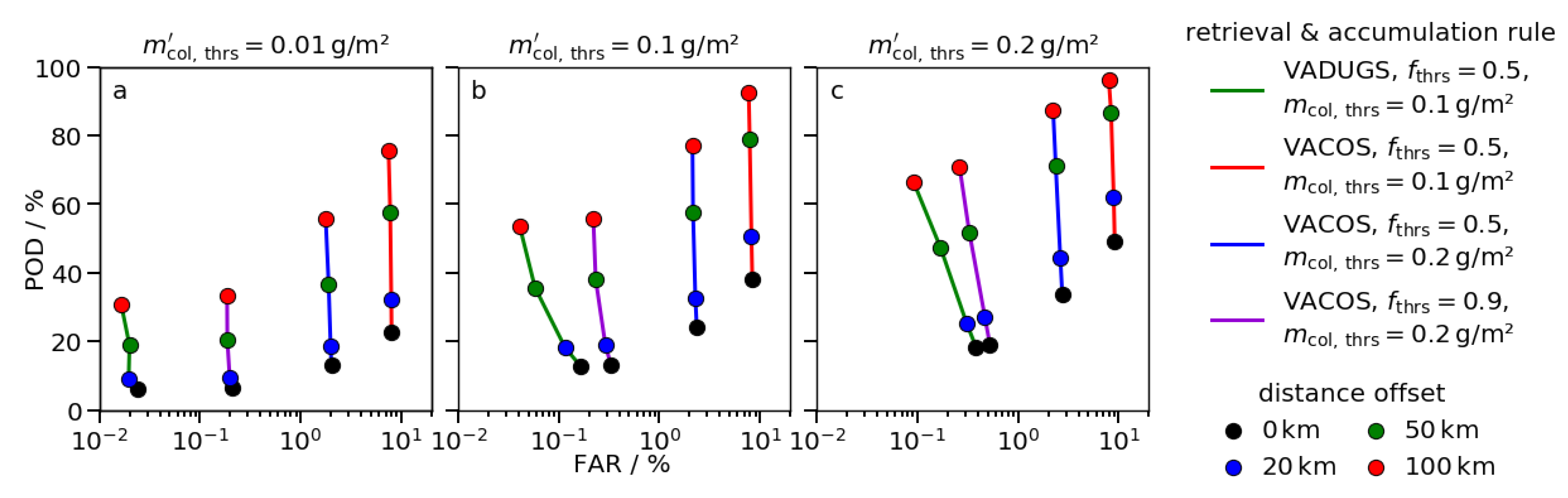
5. Comparison with a Model Ensemble
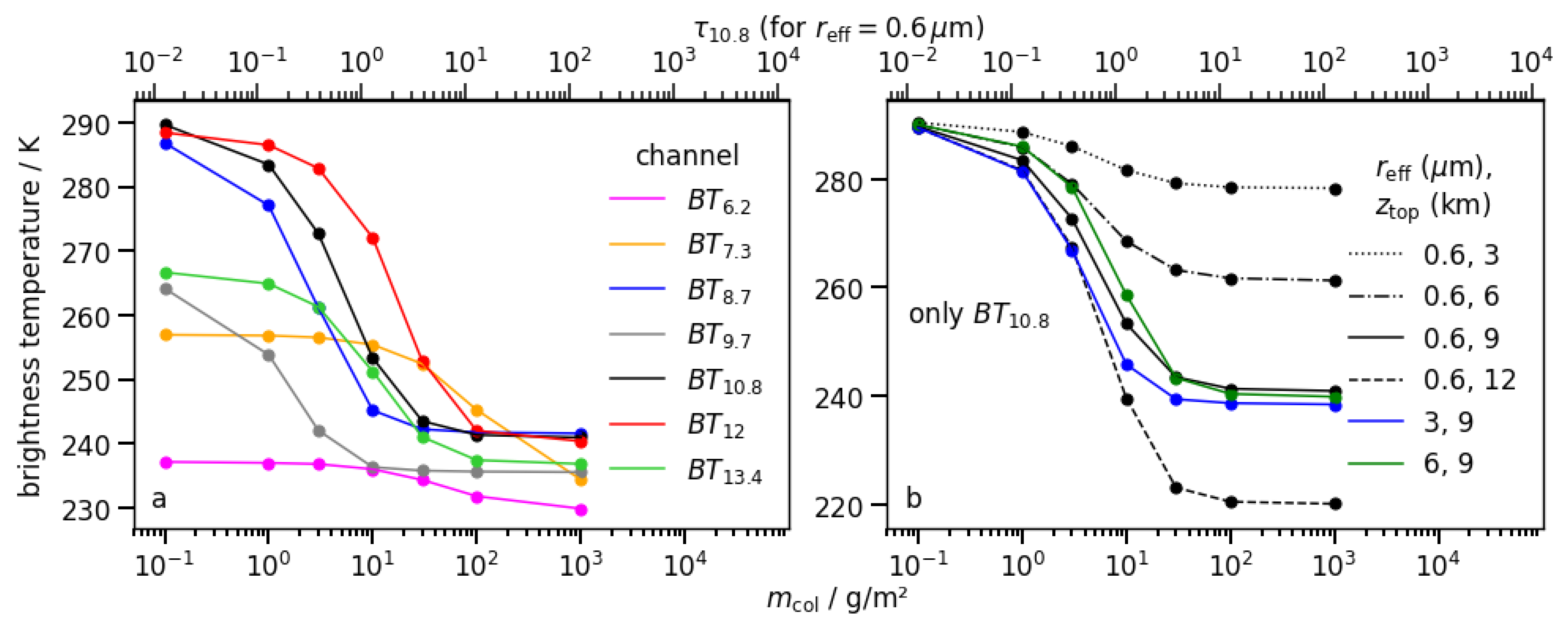
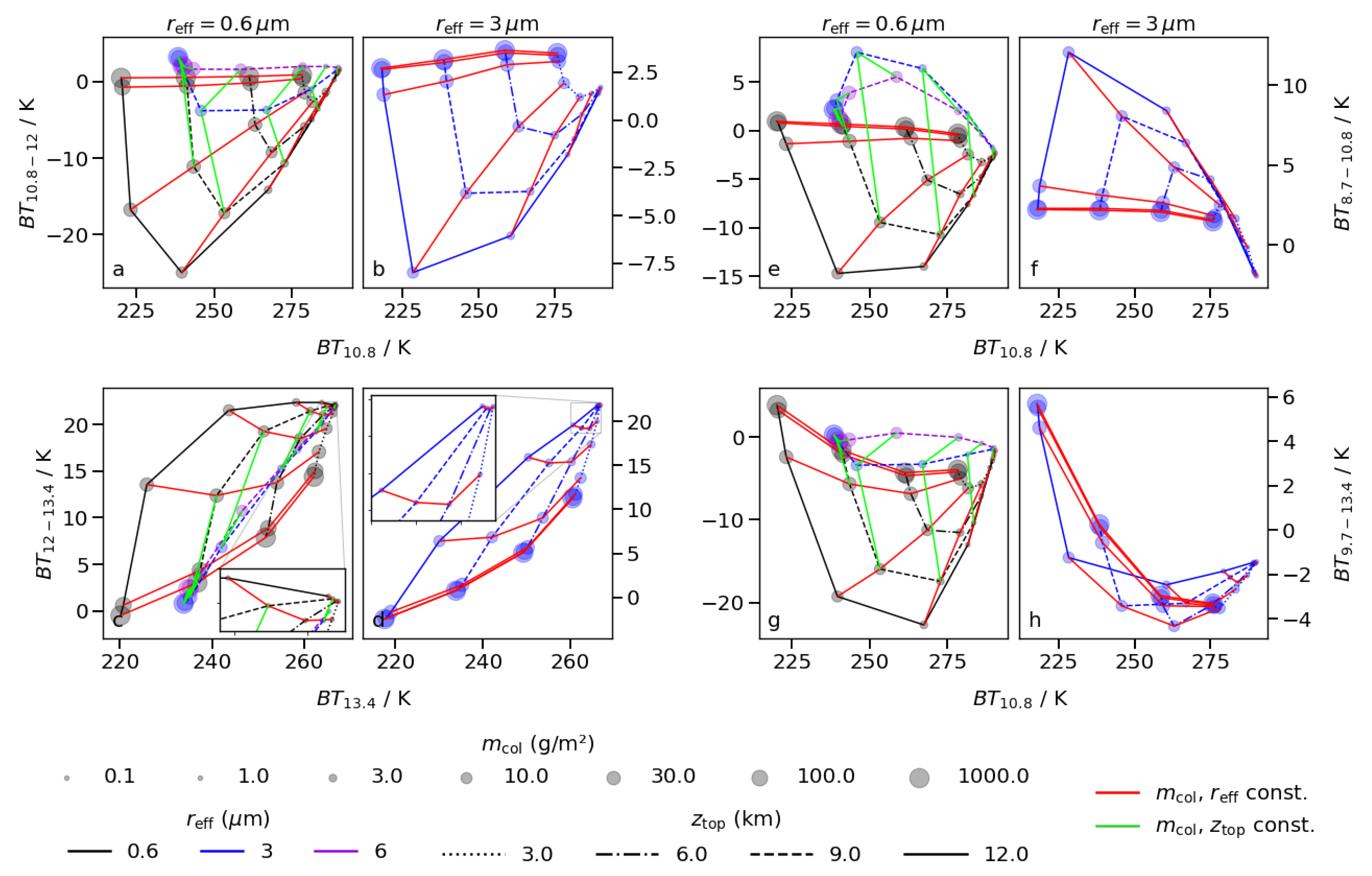
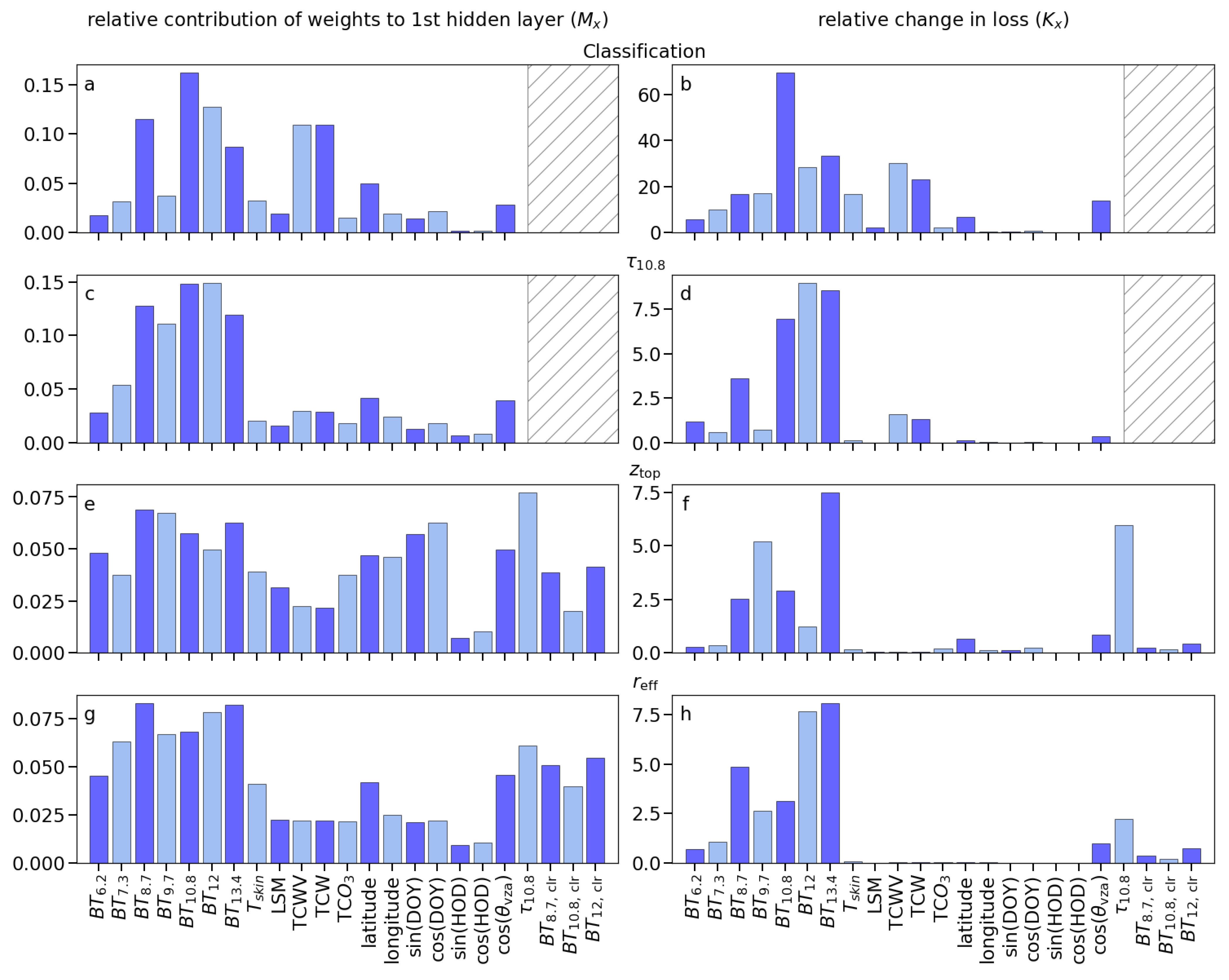
6. Unraveling the Black Box: How Do the ANNs Work?
7. Conclusions
Author Contributions
Funding
Institutional Review Board Statement
Informed Consent Statement
Data Availability Statement
Acknowledgments
Conflicts of Interest
Appendix A. Metrics
Appendix B. Π-Sigmoid Distribution
References
- Bugliaro, L.; Piontek, D.; Kox, S.; Schmidl, M.; Mayer, B.; Müller, R.; Vázquez-Navarro, M.; Gasteiger, J.; Kar, J. Combining radiative transfer calculations and a neural network for the remote sensing of volcanic ash using MSG/SEVIRI. 2021; in preparation. [Google Scholar]
- Piontek, D.; Bugliaro, L.; Schmidl, M.; Zhou, D.K.; Voigt, C. The New Volcanic Ash Retrieval VACOS Using MSG/SEVIRI and Artificial Neural Networks: 1. Development. Remote Sens. 2021, 13, 3112. [Google Scholar] [CrossRef]
- Piontek, D.; Hornby, A.; Voigt, C.; Bugliaro, L.; Gasteiger, J. Determination of complex refractive indices and optical properties of volcanic ashes in the thermal infrared based on generic petrological compositions. J. Volcanol. Geotherm. Res. 2021, 411, 107174. [Google Scholar] [CrossRef]
- Zhou, D.K.; Larar, A.M.; Liu, X.; Smith, W.L.; Strow, L.L.; Yang, P.; Schlüssel, P.; Calbet, X. Global Land Surface Emissivity Retrieved From Satellite Ultraspectral IR Measurements. IEEE Trans. Geosci. Remote Sens. 2011, 49, 1277–1290. [Google Scholar] [CrossRef]
- Zhou, D.K.; Larar, A.M.; Liu, X. MetOp-A/IASI Observed Continental Thermal IR Emissivity Variations. IEEE J. Sel. Top. Appl. Earth Obs. Remote Sens. 2013, 6, 1156–1162. [Google Scholar] [CrossRef]
- Zhou, D.K.; Larar, A.M.; Liu, X. On the relationship between land surface infrared emissivity and soil moisture. J. Appl. Remote Sens. 2018, 12, 1–14. [Google Scholar] [CrossRef] [Green Version]
- Watkin, S.C. The application of AVHRR data for the detection of volcanic ash in a Volcanic Ash Advisory Centre. Meteorol. Appl. 2003, 10, 301–311. [Google Scholar] [CrossRef]
- Kaufman, Y.J.; Koren, I.; Remer, L.A.; Rosenfeld, D.; Rudich, Y. The effect of smoke, dust, and pollution aerosol on shallow cloud development over the Atlantic Ocean. Proc. Natl. Acad. Sci. USA 2005, 102, 11207–11212. [Google Scholar] [CrossRef] [PubMed] [Green Version]
- Strandgren, J.; Bugliaro, L.; Sehnke, F.; Schröder, L. Cirrus cloud retrieval with MSG/SEVIRI using artificial neural networks. Atmos. Meas. Tech. 2017, 10, 3547–3573. [Google Scholar] [CrossRef] [Green Version]
- Strandgren, J.; Fricker, J.; Bugliaro, L. Characterisation of the artificial neural network CiPS for cirrus cloud remote sensing with MSG/SEVIRI. Atmos. Meas. Tech. 2017, 10, 4317–4339. [Google Scholar] [CrossRef] [Green Version]
- Thomas, G.E.; Stamnes, K. Radiative Transfer in the Atmosphere and Ocean, 1st ed.; Cambridge University Press: New York, NY, USA, 2002. [Google Scholar]
- de Laat, A.; Vazquez-Navarro, M.; Theys, N.; Stammes, P. Analysis of properties of the 19 February 2018 volcanic eruption of Mount Sinabung in S5P/TROPOMI and Himawari-8 satellite data. Nat. Hazards Earth Syst. Sci. 2020, 20, 1203–1217. [Google Scholar] [CrossRef]
- Schneider, D.J.; Van Eaton, A.R.; Wallace, K.L. Satellite observations of the 2016–2017 eruption of Bogoslof volcano: Aviation and ash fallout hazard implications from a water-rich eruption. Bull. Volcanol. 2020, 82, 29. [Google Scholar] [CrossRef]
- Deguine, A.; Petitprez, D.; Clarisse, L.; Guđmundsson, S.; Outes, V.; Villarosa, G.; Herbin, H. Complex refractive index of volcanic ash aerosol in the infrared, visible, and ultraviolet. Appl. Opt. 2020, 59, 884–895. [Google Scholar] [CrossRef]
- Schumann, U.; Weinzierl, B.; Reitebuch, O.; Schlager, H.; Minikin, A.; Forster, C.; Baumann, R.; Sailer, T.; Graf, K.; Mannstein, H.; et al. Airborne observations of the Eyjafjalla volcano ash cloud over Europe during air space closure in April and May 2010. Atmos. Chem. Phys. 2011, 11, 2245–2279. [Google Scholar] [CrossRef] [Green Version]
- Marenco, F.; Johnson, B.; Turnbull, K.; Newman, S.; Haywood, J.; Webster, H.; Ricketts, H. Airborne lidar observations of the 2010 Eyjafjallajökull volcanic ash plume. J. Geophys. Res. Atmos. 2011, 116. [Google Scholar] [CrossRef]
- Turnbull, K.; Johnson, B.; Marenco, F.; Haywood, J.; Minikin, A.; Weinzierl, B.; Schlager, H.; Schumann, U.; Leadbetter, S.; Woolley, A. A case study of observations of volcanic ash from the Eyjafjallajökull eruption: 1. In situ airborne observations. J. Geophys. Res. Atmos. 2012, 117. [Google Scholar] [CrossRef] [Green Version]
- Alivanoglou, A.; Likas, A. Probabilistic Models Based on the Π-Sigmoid Distribution. In Artificial Neural Networks in Pattern Recognition; Prevost, L., Marinai, S., Schwenker, F., Eds.; Springer: Berlin/Heidelberg, Germany, 2008; pp. 36–43. [Google Scholar]
- Typical Radiometric Noise, Calibration Bias and Stability for Meteosat-8, -9, -10 and -11 SEVIRI. European Organisation for the Exploitation of Meteorological Satellites. 2019. Available online: https://www-cdn.eumetsat.int/files/2020-04/pdf_typ_radiomet_acc_msg-1-2.pdf (accessed on 5 August 2021).
- Winker, D.M.; Vaughan, M.A.; Omar, A.; Hu, Y.; Powell, K.A.; Liu, Z.; Hunt, W.H.; Young, S.A. Overview of the CALIPSO Mission and CALIOP Data Processing Algorithms. J. Atmos. Ocean. Technol. 2009, 26, 2310–2323. [Google Scholar] [CrossRef]
- Kim, M.H.; Omar, A.H.; Tackett, J.L.; Vaughan, M.A.; Winker, D.M.; Trepte, C.R.; Hu, Y.; Liu, Z.; Poole, L.R.; Pitts, M.C.; et al. The CALIPSO version 4 automated aerosol classification and lidar ratio selection algorithm. Atmos. Meas. Tech. 2018, 11, 6107–6135. [Google Scholar] [CrossRef] [PubMed] [Green Version]
- Gasteiger, J.; Groß, S.; Freudenthaler, V.; Wiegner, M. Volcanic ash from Iceland over Munich: Mass concentration retrieved from ground-based remote sensing measurements. Atmos. Chem. Phys. 2011, 11, 2209–2223. [Google Scholar] [CrossRef] [Green Version]
- Winker, D.M.; Liu, Z.; Omar, A.; Tackett, J.; Fairlie, D. CALIOP observations of the transport of ash from the Eyjafjallajökull volcano in April 2010. J. Geophys. Res. Atmos. 2012, 117. [Google Scholar] [CrossRef]
- Bignami, C.; Corradini, S.; Merucci, L.; de Michele, M.; Raucoules, D.; De Astis, G.; Stramondo, S.; Piedra, J. Multisensor Satellite Monitoring of the 2011 Puyehue-Cordon Caulle Eruption. IEEE J. Sel. Top. Appl. Earth Obs. Remote Sens. 2014, 7, 2786–2796. [Google Scholar] [CrossRef]
- Ishimoto, H.; Hayashi, M.; Mano, Y. Optimal ash particle refractive index model for simulating the brightness temperature spectrum of volcanic ash clouds from satellite infrared sounder measurements. Atmos. Meas. Tech. Discuss. 2021, 2021, 1–28. [Google Scholar] [CrossRef]
- Debling, F.; Schneider, J.F.; Rosi, M.; Leoz-Garziandia, E.; Rorije, E. Technical Cooperation Mission, Effects of the Puyehue-Cordón Caulle Eruption Argentina, 4–19 July 2011. Joint UNEP/OCHA Environment Unit, 2011. Available online: https://www.eecentre.org/wp-content/uploads/2019/06/Argentina-volcan-eruption-2011-report.pdf (accessed on 5 August 2021).
- Botto, I.L.; Canafoglia, M.E.; Gazzoli, D.; González, M.J. Spectroscopic and Microscopic Characterization of Volcanic Ash from Puyehue-(Chile) Eruption: Preliminary Approach for the Application in the Arsenic Removal. J. Spectrosc. 2013, 2013, 254517. [Google Scholar] [CrossRef] [Green Version]
- Johnson, B.; Turnbull, K.; Brown, P.; Burgess, R.; Dorsey, J.; Baran, A.J.; Webster, H.; Haywood, J.; Cotton, R.; Ulanowski, Z.; et al. In situ observations of volcanic ash clouds from the FAAM aircraft during the eruption of Eyjafjallajökull in 2010. J. Geophys. Res. Atmos. 2012, 117. [Google Scholar] [CrossRef] [Green Version]
- Ball, J.G.C.; Reed, B.E.; Grainger, R.G.; Peters, D.M.; Mather, T.A.; Pyle, D.M. Measurements of the complex refractive index of volcanic ash at 450, 546.7, and 650 nm. J. Geophys. Res. Atmos. 2015, 120, 7747–7757. [Google Scholar] [CrossRef]
- Weber, K.; Eliasson, J.; Vogel, A.; Fischer, C.; Pohl, T.; van Haren, G.; Meier, M.; Grobéty, B.; Dahmann, D. Airborne in situ investigations of the Eyjafjallajökull volcanic ash plume on Iceland and over north-western Germany with light aircrafts and optical particle counters. Atmos. Environ. 2012, 48, 9–21. [Google Scholar] [CrossRef]
- Gudmundsson, M.T.; Thordarson, T.; Höskuldsson, A.; Larsen, G.; Björnsson, H.; Prata, F.J.; Oddsson, B.; Magnússon, E.; Högnadóttir, T.; Petersen, G.N.; et al. Ash generation and distribution from the April-May 2010 eruption of Eyjafjallajökull, Iceland. Sci. Rep. 2012, 2, 572. [Google Scholar] [CrossRef] [Green Version]
- Rose, W.; Gu, Y.; Watson, I.; Yu, T.; Blut, G.; Prata, A.; Krueger, A.; Krotkov, N.; Carn, S.; Fromm, M.; et al. The February–March 2000 Eruption of Hekla, Iceland from a Satellite Perspective. In Volcanism and the Earth’s Atmosphere; American Geophysical Union: Washington, DC, USA, 2004; pp. 107–132. [Google Scholar] [CrossRef] [Green Version]
- Rose, W.I.; Bluth, G.J.S.; Watson, I.M. Ice in Volcanic Clouds: When and Where? In Proceedings of the 2nd International Conference on Volcanic Ash and Aviation Safety, Alexandria, VA, USA, 21–24 June 2004; Office of the Federal Coordinator for Meteorological Services and Supporting Research: Silver Spring, MD, USA, 2004; pp. 3.27–3.33. [Google Scholar]
- Durant, A.J.; Shaw, R.A.; Rose, W.I.; Mi, Y.; Ernst, G.G.J. Ice nucleation and overseeding of ice in volcanic clouds. J. Geophys. Res. Atmos. 2008, 113. [Google Scholar] [CrossRef] [Green Version]
- Plu, M.; Scherllin-Pirscher, B.; Arnold Arias, D.; Baro, R.; Bigeard, G.; Bugliaro, L.; Carvalho, A.; El Amraoui, L.; Eschbacher, K.; Hirtl, M.; et al. A tailored multi-model ensemble for air traffic management: Demonstration and evaluation for the Eyjafjallajökull eruption in May 2010. Nat. Hazards Earth Syst. Sci. Discuss. 2021, 2021, 1–32. [Google Scholar] [CrossRef]
- Kox, S.; Bugliaro, L.; Ostler, A. Retrieval of cirrus cloud optical thickness and top altitude from geostationary remote sensing. Atmos. Meas. Tech. 2014, 7, 3233–3246. [Google Scholar] [CrossRef] [Green Version]
- Prata, A.J. Infrared radiative transfer calculations for volcanic ash clouds. Geophys. Res. Lett. 1989, 16, 1293–1296. [Google Scholar] [CrossRef]
- Wen, S.; Rose, W.I. Retrieval of sizes and total masses of particles in volcanic clouds using AVHRR bands 4 and 5. J. Geophys. Res. Atmos. 1994, 99, 5421–5431. [Google Scholar] [CrossRef]
- LeCun, Y.; Denker, J.S.; Solla, S.A. Optimal Brain Damage. In Advances in Neural Information Processing Systems 2; Touretzky, D.S., Ed.; Morgan-Kaufmann: San Francisco, CA, USA, 1990; pp. 598–605. [Google Scholar]
- Piscini, A.; Carboni, E.; Del Frate, F.; Grainger, R.G. Simultaneous retrieval of volcanic sulphur dioxide and plume height from hyperspectral data using artificial neural networks. Geophys. J. Int. 2014, 198, 697–709. [Google Scholar] [CrossRef] [Green Version]
- Ackerman, S.A. Remote sensing aerosols using satellite infrared observations. J. Geophys. Res. Atmos. 1997, 102, 17069–17079. [Google Scholar] [CrossRef]
- Gray, T.M.; Bennartz, R. Automatic volcanic ash detection from MODIS observations using a back-propagation neural network. Atmos. Meas. Tech. 2015, 8, 5089–5097. [Google Scholar] [CrossRef] [Green Version]
- Schmit, T.J.; Gunshor, M.M.; Menzel, W.P.; Gurka, J.J.; Li, J.; Bachmeier, A.S. Introducing the Next-Generation Advanced Baseline Imager on GOES-R. Bull. Am. Meteorol. Soc. 2005, 86, 1079–1096. [Google Scholar] [CrossRef]
- Bessho, K.; Date, K.; Hayashi, M.; Ikeda, A.; Imai, T.; Inoue, H.; Kumagai, Y.; Miyakawa, T.; Murata, H.; Ohno, T.; et al. An Introduction to Himawari-8/9 - Japan’s New-Generation Geostationary Meteorological Satellites. J. Meteorol. Soc. Jpn. Ser. II 2016, 94, 151–183. [Google Scholar] [CrossRef] [Green Version]
- Yang, J.; Zhang, Z.; Wei, C.; Lu, F.; Guo, Q. Introducing the New Generation of Chinese Geostationary Weather Satellites, Fengyun-4. Bull. Am. Meteorol. Soc. 2017, 98, 1637–1658. [Google Scholar] [CrossRef]
- Meeting on the Intercomparison of Satellite-Based Volcanic Ash Retrieval Algorithms, Madison WI, USA, 29 June–2 July 2015, Final Report. World Meteorological Organization, 2015. Available online: https://web.archive.org/web/20171113102551/http://www.wmo.int/pages/prog/sat/documents/SCOPE-NWC-PP2_VAIntercompWSReport2015.pdf (accessed on 5 August 2021).
- Stohl, A.; Prata, A.J.; Eckhardt, S.; Clarisse, L.; Durant, A.; Henne, S.; Kristiansen, N.I.; Minikin, A.; Schumann, U.; Seibert, P.; et al. Determination of time- and height-resolved volcanic ash emissions and their use for quantitative ash dispersion modeling: The 2010 Eyjafjallajökull eruption. Atmos. Chem. Phys. 2011, 11, 4333–4351. [Google Scholar] [CrossRef] [Green Version]
- Dacre, H.F.; Harvey, N.J.; Webley, P.W.; Morton, D. How accurate are volcanic ash simulations of the 2010 Eyjafjallajökull eruption? J. Geophys. Res. Atmos. 2016, 121, 3534–3547. [Google Scholar] [CrossRef] [Green Version]
- Plu, M.; Bigeard, G.; Sič, B.; Emili, E.; Bugliaro, L.; El Amraoui, L.; Guth, J.; Josse, B.; Mona, L.; Piontek, D. Modelling the volcanic ash plume from Eyjafjallajökull eruption (May 2010) over Europe: Evaluation of the benefit of source term improvements and of the assimilation of aerosol measurements. Nat. Hazards Earth Syst. Sci. Discuss. 2021, 2021, 1–24. [Google Scholar] [CrossRef]
- Barnes, L.R.; Schultz, D.M.; Gruntfest, E.C.; Hayden, M.H.; Benight, C.C. CORRIGENDUM: False Alarm Rate or False Alarm Ratio? Weather Forecast. 2009, 24, 1452–1454. [Google Scholar] [CrossRef] [Green Version]


| Retrieval/% | |||||
|---|---|---|---|---|---|
| Truth | Samples | Clear | Clouds | Ash | Both |
| clear | 560,713 | 99.7 | 0.3 | <0.1 | <0.1 |
| clouds | 287,740 | 5.6 | 94.3 | <0.1 | <0.1 |
| ash | 279,395 | <0.1 | <0.1 | 94.6 | 5.2 |
| both | 124,622 | <0.1 | 4.1 | 46.8 | 49.2 |
| Retrieval/% | |||||
|---|---|---|---|---|---|
| Cloud Location | Samples | Clear | Clouds | Ash | Both |
| above | 21,833 | <0.1 | 15.1 | 48.8 | 36.1 |
| below | 81,630 | <0.1 | 0.3 | 48.0 | 51.6 |
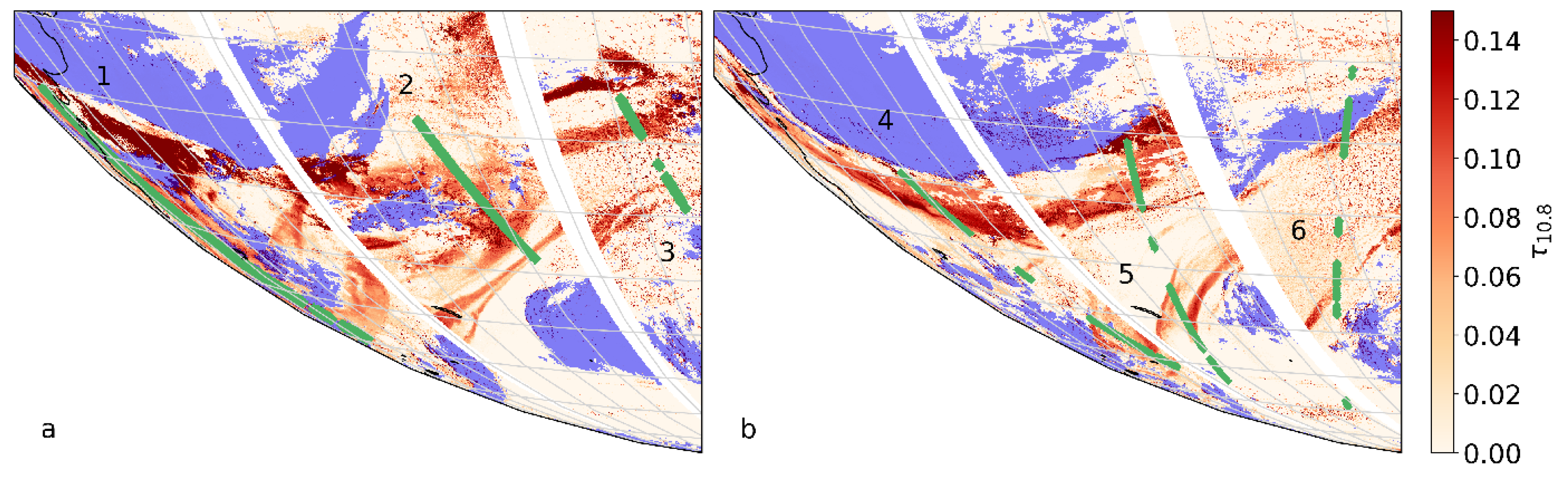
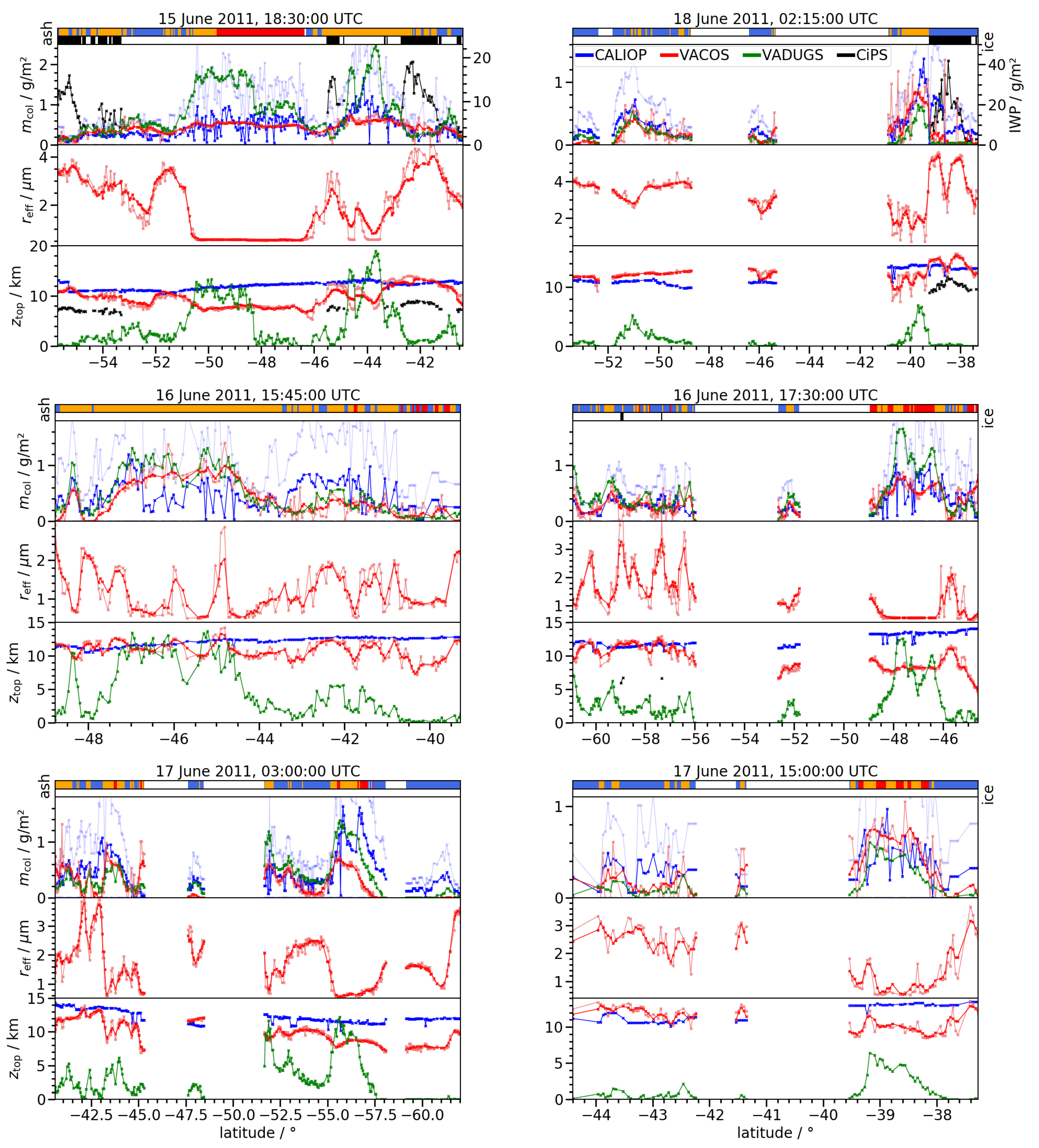
| Day | Start Time/UTC | End Time/UTC | Start Coordinates | End Coordinates | Samples | Track Number |
|---|---|---|---|---|---|---|
| 15 June 2011 | 18:30 | 18:40 | N, E | N, E | 300 | 1 |
| 16 June 2011 | 15:51 | 16:05 | N, E | N, E | 162 | 2 |
| 16 June 2011 | 17:29 | 17:43 | N, E | N, E | 187 | 4 |
| 17 June 2011 | 03:00 | 03:13 | N, E | N, E | 251 | 5 |
| 17 June 2011 | 14:55 | 15:10 | N, E | N, E | 82 | 3 |
| 18 June 2011 | 02:04 | 02:18 | N, E | N, E | 199 | 6 |
| Algorithm | MAPE | MPE | MAPE | MPE |
| full data set (1181 samples) | ||||
| VADUGS | 123% | 70% | 75% | % |
| VACOS (1 px) | 190% | 93% | 19% | % |
| VACOS (9 px) | 111% | 43% | 18% | % |
| VACOS (25 px) | 112% | 49% | 18% | % |
| only (875 samples) | ||||
| VADUGS | 62% | 12% | 71% | % |
| VACOS (1 px) | 56% | % | 18% | % |
| VACOS (9 px) | 47% | % | 18% | % |
| VACOS (25 px) | 45% | % | 18% | % |
| Algorithm | Accumulation Rule | ≥ 0.01 g m | ≥ 0.2 g m | and ≥ 0.2 g m | ||||||
|---|---|---|---|---|---|---|---|---|---|---|
| (; ) | Samples | MAPE | MPE | Samples | MAPE | MPE | samples | MAPE | MPE | |
| VADUGS | 0.1 g m−2; 0.5 | 222,932 | 99% | % | 63,595 | 94% | % | 6201 | 65% | % |
| VACOS | 0.1 g m−2; 0.5 | 221,663 | 138% | % | 63,363 | 79% | % | 26,200 | 57% | 0% |
| VACOS | 0.2 g m−2; 0.5 | 221,633 | 127% | % | 63,357 | 87% | % | 21,331 | 60% | 12% |
| VACOS | 0.2 g m−2; 0.9 | 221,663 | 106% | % | 63,363 | 94% | % | 12,006 | 68% | 25% |
Publisher’s Note: MDPI stays neutral with regard to jurisdictional claims in published maps and institutional affiliations. |
© 2021 by the authors. Licensee MDPI, Basel, Switzerland. This article is an open access article distributed under the terms and conditions of the Creative Commons Attribution (CC BY) license (https://creativecommons.org/licenses/by/4.0/).
Share and Cite
Piontek, D.; Bugliaro, L.; Kar, J.; Schumann, U.; Marenco, F.; Plu, M.; Voigt, C. The New Volcanic Ash Satellite Retrieval VACOS Using MSG/SEVIRI and Artificial Neural Networks: 2. Validation. Remote Sens. 2021, 13, 3128. https://doi.org/10.3390/rs13163128
Piontek D, Bugliaro L, Kar J, Schumann U, Marenco F, Plu M, Voigt C. The New Volcanic Ash Satellite Retrieval VACOS Using MSG/SEVIRI and Artificial Neural Networks: 2. Validation. Remote Sensing. 2021; 13(16):3128. https://doi.org/10.3390/rs13163128
Chicago/Turabian StylePiontek, Dennis, Luca Bugliaro, Jayanta Kar, Ulrich Schumann, Franco Marenco, Matthieu Plu, and Christiane Voigt. 2021. "The New Volcanic Ash Satellite Retrieval VACOS Using MSG/SEVIRI and Artificial Neural Networks: 2. Validation" Remote Sensing 13, no. 16: 3128. https://doi.org/10.3390/rs13163128