Abstract
Shrinking cities—cities suffering from population and economic decline—has become a pressing societal issue of worldwide concern. While night-time light (NTL) data have been applied as an important tool for the identification of shrinking cities, the current methods are constrained and biased by the lack of using long-term continuous NTL time series and the use of unidimensional indices. In this study, we proposed a novel method to identify and classify shrinking cities by long-term continuous NTL time series and population data, and applied the method in northeastern China (NEC) from 1996 to 2020. First, we established a long-term consistent NTL time series by applying a geographically weighted regression model to two distinct NTL datasets. Then, we generated NTL index (NI) and population index (PI) by random forest model and the slope of population data, respectively. Finally, we developed a shrinking city index (SCI), based on NI and PI to identify and classify city shrinkage. The results showed that the shrinkage pattern of NEC in 1996–2009 (stage 1) and 2010–2020 (stage 2) was quite different. From stage 1 to stage 2, the shrinkage situation worsened as the number of shrinking cities increased from 102 to 162, and the proportion of severe shrinkage increased from 9.2% to 30.3%. In stage 2, 85.4% of the cities exhibited population decline, and 15.7% of the cities displayed an NTL decrease, suggesting that the changes in NTL and population were not synchronized. Our proposed method provides a robust and long-term characterization of city shrinkage and is beneficial to provide valuable information for sustainable urban planning and decision-making.
1. Introduction
Shrinking city, a term proposed in the early 1990s [1], refers to cities suffering from population and economic decline. City shrinkage has been identified in more than a quarter of the world’s cities, and this percentage is still rising [2], particularly in developed countries [3,4,5,6]. Wolff et al. [7] confirmed that 54% of the urban areas in Europe were experiencing population loss. Pallagst et al. [8] noted that 13% of the urban regions in the US shrank, among which many historical industrial cities, such as Detroit, were in the most serious condition [9]. Recently, shrinking cities have also been found in developing countries [10,11,12]. Among them, cities in northeastern China where old industrial bases are located were typical cases [13,14]. City shrinkage has a profound impact on economic development, social differentiation, urban renewal, government decision-making, infrastructure construction and urban planning development; thus, this phenomenon has received increasing attention worldwide in recent decades [15,16,17,18,19].
Early studies mainly focused on the definition of city shrinkage. As population decrease is the most representative characteristic of shrinking cities, it is normally used as the main indicator for quantifying shrinking cities. Wiechmann et al. [19] defined cities with a continuous population decline for more than two years as shrinking cities. Oswalt et al. [20] identified shrinking cities by a more than 10% decrease in the total population or more than 1% average rate of decline in the population. Considering that there are many other features of city shrinkage, such as economic decline, declines in the urban living environment and increased housing vacancy rates, more comprehensive definitions have been gradually adopted. Schilling et al. [21] incorporated the increase in the housing vacancy rate into a definition of shrinkage based on population loss. Because economic decline is very important, Bartholomae et al. [22] redefined the phenomenon based on the population and economic activities. The classification of shrinking cities has also been researched, and scholars have taken different perspectives. Alves et al. [23] classified shrinking cities into five types, according to the different stages in the population loss process. Bartholomae et al. [22] incorporated population change and economic activity change to categorize four types of cities. Extensive efforts have been made to determine the driving factors of city shrinkage, including population ageing [5], resource depletion [24], climate change [25], and deindustrialization [26]. Although some progress has been made, city shrinkage is still a challenging issue for decision makers due to its complexity [27]. Researchers are still trying to reveal the underlying mechanism of urban development and thus better support government decision-making in the context of city shrinkage.
To study city shrinkage, it is of primary importance to design an appropriate framework for identifying these cities. Unfortunately, a well-acknowledged standard is still scarce [28]. Most previous studies used population loss based on census data as a single index for identification [2,7,8,20]; however, these frameworks have been criticized for their biased representations. Night-time light (NTL) data recorded by satellite have been confirmed to be highly related to demographic and socioeconomic variables, such as the gross domestic product (GDP), population density, energy consumption, and urban area detection from the global to pixel levels [29,30,31,32]. Compared with conventional statistical data, NTL data can reflect actual human activities directly at a finer resolution [33]. A few studies have applied NTL data to identify shrinking cities and provided valuable experience [34,35,36]. However, there were several noteworthy drawbacks to these studies, among which the lack of continuous long-term time series was a main problem. Given that city shrinkage is a gradual process, previous NTL-based studies only focused on a short period of time or even a single year [27,34,37]. With data from limited time nodes, the continuous changes in city shrinkage cannot be revealed. More importantly, the instability of a single temporal observation impairs the robustness of the results. Moreover, city shrinkage is not a constant process and has multiple stages. Different stages may have different driving forces and display different characteristics. Single sets of temporal data cannot be used in stage division, stage analysis or transformation analysis, which are meaningful in city shrinkage research. In comparison, continuous time series data are able to uncover long-term NTL patterns and thereby provide creditable characterizations of rapid socioeconomic changes. Previous studies did not apply long-term continuous NTL data, mainly due to the inconsistency between the two most commonly used NTL sensors: the Defense Meteorological Satellite Program’s Operational Linescan System (DMSP-OLS) and the National Polar-orbiting Partnership Visible Infrared Imaging Radiometer Suite (NPP/VIIRS) [38]. Although DMSP/OLS extension data were released recently, the lack of time extendibility, inappropriate overpass time and poor data quality constrained its application. Thus, it is still necessary to apply cross-sensor calibration on DMSP and NPP/VIIRS.
Another key drawback of the existing methods is that as sophisticated as shrinking cities are, they were mostly identified unidimensionally by a single NTL index [27,34]. Few studies have combined NTL data with other auxiliary variables. A single indicator can only reflect one aspect of shrinkage. Without multiple indices, it is difficult to comprehensively describe the characteristics of shrinking cities, and variations among different factors cannot be identified, thus limiting detailed analysis. In addition, the construction of an NTL index in most previous studies was merely based on the average digital number (DN) value [27,36]. There are many NTL features at the regional scale, but little attention has been given to selecting representative features to generate a comprehensive indicator. This limitation may cause some information related to classifying shrinking cities with NTL data to not be thoroughly extracted.
To fill these research gaps, this study proposed a novel method to identify and classify shrinking cities by combining long-term time series of NTL data from 1996 to 2020 with auxiliary data. To achieve these goals, we (1) cross-calibrated different NTL sensors and generated long-term consistent NTL time series; (2) developed robust standards to identify and classify shrinking cities based on multiple variables; and (3) analyzed the spatiotemporal patterns of shrinking cities. This study aims to reveal the long-term characteristics of city shrinkage by using continuous sets of NTL data and auxiliary data and provides valuable insight for government decision makers regarding shrinking city development.
2. Study Area and Datasets
2.1. Study Area
Heilongjiang, Jilin and Liaoning, three provinces in northeastern China (NEC), were selected as the study area (Figure 1). Benefitted by vast plains and rich resources, this region started its urbanization at an early age. NEC includes 34 prefecture-level cities today and covers an area of 806,100 km2. Considering the access to statistical data, we chose county (district) level as the research scale. We merged all the districts belonging to a specific prefecture level city and used the prefecture city’s name to name its corresponding merged districts. Thus, the basic unit of our study consists of three parts: county, county-level city and merged districts. We made some adjustments to assure that statistical data in the whole period matched the administrative boundary. To be specific, the population and GDP of withdrawn counties (districts) were allocated into the surrounding cities by using the county (district)-level administrative boundary of the NEC in 2018 as standard. We finally obtained 185 basic study unites. Among them, 9 cities are big cities (urban resident population is over 1 million), 17 cities are medium cities (urban resident population is between 0.5 million and 1 million), and others are small cities (urban resident population is less than 0.5 million).
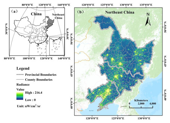
Figure 1.
(a) Location of the study area; (b) NTL radiance (nW/cm2/sr) in 2020.
NEC was known as the old industrial basement of China and used to be an important pillar of China’s economy. Many of the cities in NEC are important resource-based industrial cities such as Fushun, Anshan, Jixi and Hegang, and the economy of these cities are severely dependent on heavy industry. Exemplified by Fushun, the value added of the second industry accounts for 43% of its GDP in 2018. In recent decades, due to resource exhaustion and global economic downturns, many of the cities in these provinces have suffered from population decline and economic recession. According to the China National Statistical Yearbooks, the total population in NEC decreased from 109.7 million in 2012 to 105.8 million in 2018 [39,40], while the national population increased rapidly during the same period. In terms of the economy, the total GDP of NEC in 2018 was USD 8812.1 billion with a growth rate of 5.5%; both were lower than the national average level. Therefore, NEC are ideal sites to study city shrinkage and test our method.
2.2. Datasets
The datasets used in the study are summarized in Table 1, which include NTL data, social census data and human settlement data. NTL data include the global radiance-calibrated DMSP-OLS (DMSPgrc) and NPP/VIIRS products. DMSPgrc are yearly composites with a spatial resolution of 30 arc-seconds. Compared to the frequently used stable light product of DMSP-OLS, DMSPgrc products have better data quality. By combining sparse data obtained at low-gain settings with the operational data obtained at high-gain settings, the dynamic range of DMSPgrc was improved, and the saturation effects were eliminated [38]. DMSPgrc were only available for eight years, 1996, 1999, 2000, 2003, 2004, 2006, 2010 and 2011, and all the data in these years were included in this study. Version 2 (V2) yearly composite VIIRS data were collected from 2012 to 2020. VIIRS provide NTL measurements in radiance and have a higher spatial resolution of 15 arc-seconds than DMSP. The effects of lunar illumination, stray light, lightning and cloud cover were eliminated [33]. Compared to Version 1 VIIRS monthly data, the V2 annually VIIRS data applied outlier removal to exclude background noise [41]. Social census data, including population data and GDP data at the county scale, were collected from the China Statistical Yearbook. To further analyze the land expansion condition in shrinking cities, we used human settlement data produced by Gong et al. [42]. The data have a resolution of 30 m and an overall accuracy of 90%.

Table 1.
Datasets and description.
3. Methodology
In this paper, “city shrinkage” was defined as a phenomenon in which a city experiences either an NTL decline or a population decrease in a certain stable period. The rationale of using population data from censuses instead of population grids based on remote sensing (e.g., Landscan) was that population grids based on remote sensing are more unstable at the regional scale than population data based on censuses. The method comprised three parts: (1) building consistent long-term time series (from 1996 to 2020) of NTL data based on DMSPgrc data and VIIRS data, (2) identifying shrinking cities and (3) classifying shrinking cities. Figure 2 shows the flowchart of this study.
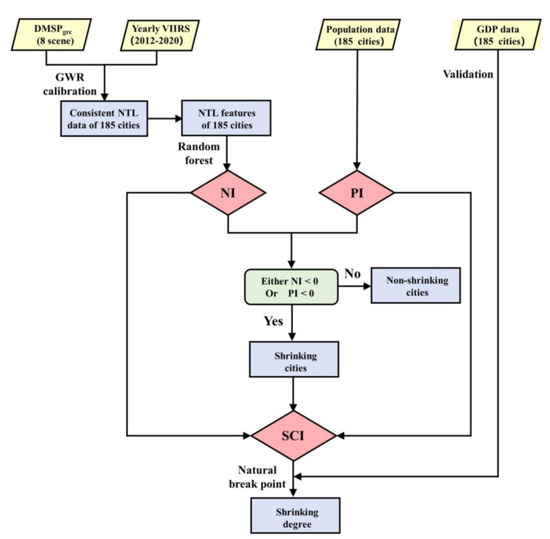
Figure 2.
Flowchart of this study (NI refers to the NTL index, PI refers to the population index and SCI refers to the shrinking city index).
3.1. Data Pre-Processing
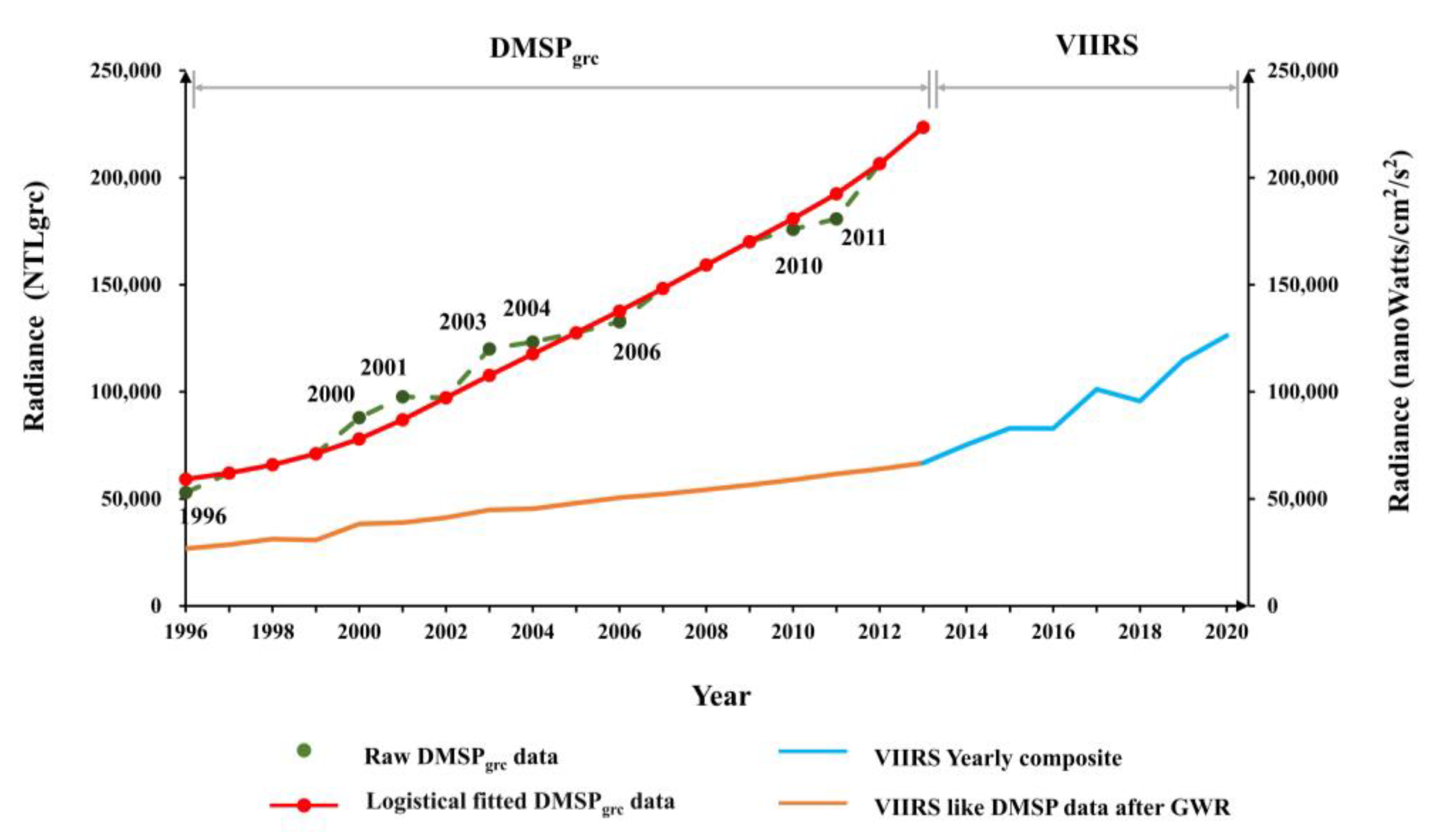
There were two tasks in the pre-processing stage: (1) DMSPgrc and VIIRS data cross-sensor calibration and (2) trend assessment for both datasets followed by stage division, if necessary. Geographically weighted regression (GWR) was chosen as the cross-sensor calibration method; GWR is a commonly used regression model that considers spatial non-stationarity [43] and has been proven to be effective in the calibration of NTL data [38]. A schematic diagram of the whole process is shown in Figure 3.

Figure 3.
Schematic diagram of NTL data pre-processing.
In the pre-processing of DMSPgrc data, first, saturation effects and geometric errors were excluded, and the invariant region method was then applied for inter-calibration. DMSPgrc only include data for eight years, and thus, a logistical model was used to estimate data for the remaining years from 1996 to 2013. The expression is as follows:
where DMSPgrc is the DN value of a specific pixel, e is the base of the natural logarithm, t is the year, and a, b, c, d are logistical regression coefficients, and they were determined by iterating the parameters continuously until the optimal group was reached; the fitted data were labeled as DMSPgrc’. Considering that the fitting effect of some pixels may have estimation errors, pixels within fitting curves that have a coefficient of determination (R2) lower than 0.85 were replaced by the average of the surrounding eight pixels according to Zheng et al. [38]. Although most of the background noises of the V2 VIIRS data have been removed [41], we made some pre-processing to further improve the data. Since Shenyang, Changchun and Harbin are the three biggest and most developed cities in NEC, the pixel values of the other areas in NEC should not exceed these cities. The highest DN value of those three cities in every year was used as a threshold to correct the outliers. In addition, values less than zero or other extreme values were removed. Then, the GWR model was applied to DMSPgrc’ (resampled to 500 m) and VIIRS in the overlapping years 2012 and 2013; the GWR expression is as follows:
where and denote the spatial location of the ith pixel, and stand for the intercept and slope, respectively, and indicate the DN value of VIIRS and DMSPgrc’ and is the residual of the model. By applying the regression coefficients for all other years, NTL data for a complete time series from 1996 to 2020 with a resolution of 500 m were finally obtained.
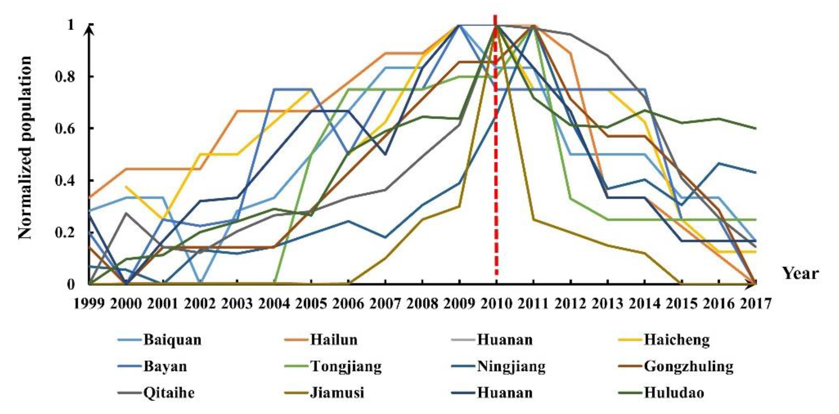
The trends of both datasets were checked, and we found that although the light curves did not display an obvious trend, most of the city population trajectories exhibited a noticeable two-stage pattern in which the population increased initially and declined afterwards (Figure 4). It is worth noting that the population peaks in 125 cities, accounting for 67.8% of all the cities studied, appeared between 2009 and 2011. Considering that a serious world financial crisis occurred in 2008, it is reasonable to assume that the city shrinkage in NEC was affected by this crisis [13]. Previous studies also noted that cities in NEC entered a transition period in 2010 [13]. Therefore, we divided the time series into two stages: S1 (1996–2009) and S2 (2010–2020).
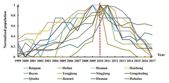
Figure 4.
Population curves of some of the cities in NEC.
3.2. Construction of the NTL Index (NI) and Population Index (PI)
Reasonable quantitative indices must be established to identify shrinking cities via long-term time series of population data and NTL data. We generated the following indices in this study.
- (1)
- NTL index (NI)
NTL data have many feature values, but most previous studies only chose the average DN as the indicator for identifying shrinking cities. In this study, a random forest (RF) method was applied to search the NTL features with the highest discrimination abilities for shrinking cities. The RF approach is a classic machine learning method that uses multiple trees for training and sample prediction and has been widely used in classification [44]. We calculated eight candidate NTL features, including the slope of the total DN, the intercept of the total DN, the slope of the average DN, the intercept of the average DN, the slope of the top 10% of DN values, the intercept of the top 10% of DN values, the slope of light pixel areas and the intercept of light pixel areas. Since there is no recognized shrinking city dataset, ten typical shrinking cities and thirty non-shrinking cities identified by Long et al. [12] were chosen as training samples. Notably, Long et al. [12] used census data to identify shrinking cities in China, and the results of their study have been supported by many related studies. The population census data and the GDP data for the ten typical shrinking cities were further checked to ensure their representativeness as shrinking cities. The R2 was used to judge the accuracy of the model, and the out-of-bag (OOB) error was used to assess the relative importance of all features. According to experience, NTL features with a normalized OOB higher than 0.5 were chosen as important features. Then, the NI was constructed by using the selected features to calculate modular distance:
where denotes the number of selected features, , …, and are the top-n features of highest importance (all normalized) and , , and are the weights. Here, we used the reciprocals of the OOB errors as the weights for different features. For a specific city, if either of the value of the selected features is negative, we define the NI of this city is negative, otherwise it is positive.
- (2)
- Population index (PI)
We defined the slope changes for the registered residence population in each city during a period by the PI (population index):
where denotes the ith year, denotes the average over all years, denotes the population in the ith year and denotes the average population in the whole period.
3.3. Shrinking City Classification
Based on the characteristics of the NI and PI in a given period, all the cities were divided into four categories marked as non-shrinkage (the value of NI is positive, and the value of PI is positive), P-shrinkage (the value of NI is positive, and the value of PI is negative), N-shrinkage (the value of NI is negative, and the value of PI is positive) and NP-shrinkage (the value of NI is negative, and the value of PI is negative). To further evaluate the severity of city shrinkage, the shrinking city index (SCI) was established to combine the PI and NI and reflect the degree of shrinkage according to the modular distance between the two indices:
where NI is the NTL index and expresses NTL shrinkage and PI is the population index and reflects population shrinkage (all normalized). After the SCI values of all the cities were calculated, the natural breaks method was used to categorize the cities into three levels: slight shrinkage, medium shrinkage and severe shrinkage. Whether an indicator can appropriately reflect the characteristics of shrinking cities is mainly determined by its sensitivity to population decreases and declines in economic activities. Considering that the SCI was generated from the PI, the SCI itself can reflect population declines. Thus, we need to verify the consistency of this index with changes of economic activities to further test its robustness. GDP data were applied to express the economic activities of the cities, and the slope of changes in each city’s GDP during a period were calculated as the GI (GDP index):
where denotes the ith year, denotes the average over all years, denotes the GDP in the ith year and denotes the average GDP in the whole period. Then, linear regression was used to verify the consistency of the two indices.
4. Results
4.1. Performance Assessment of the Proposed Method
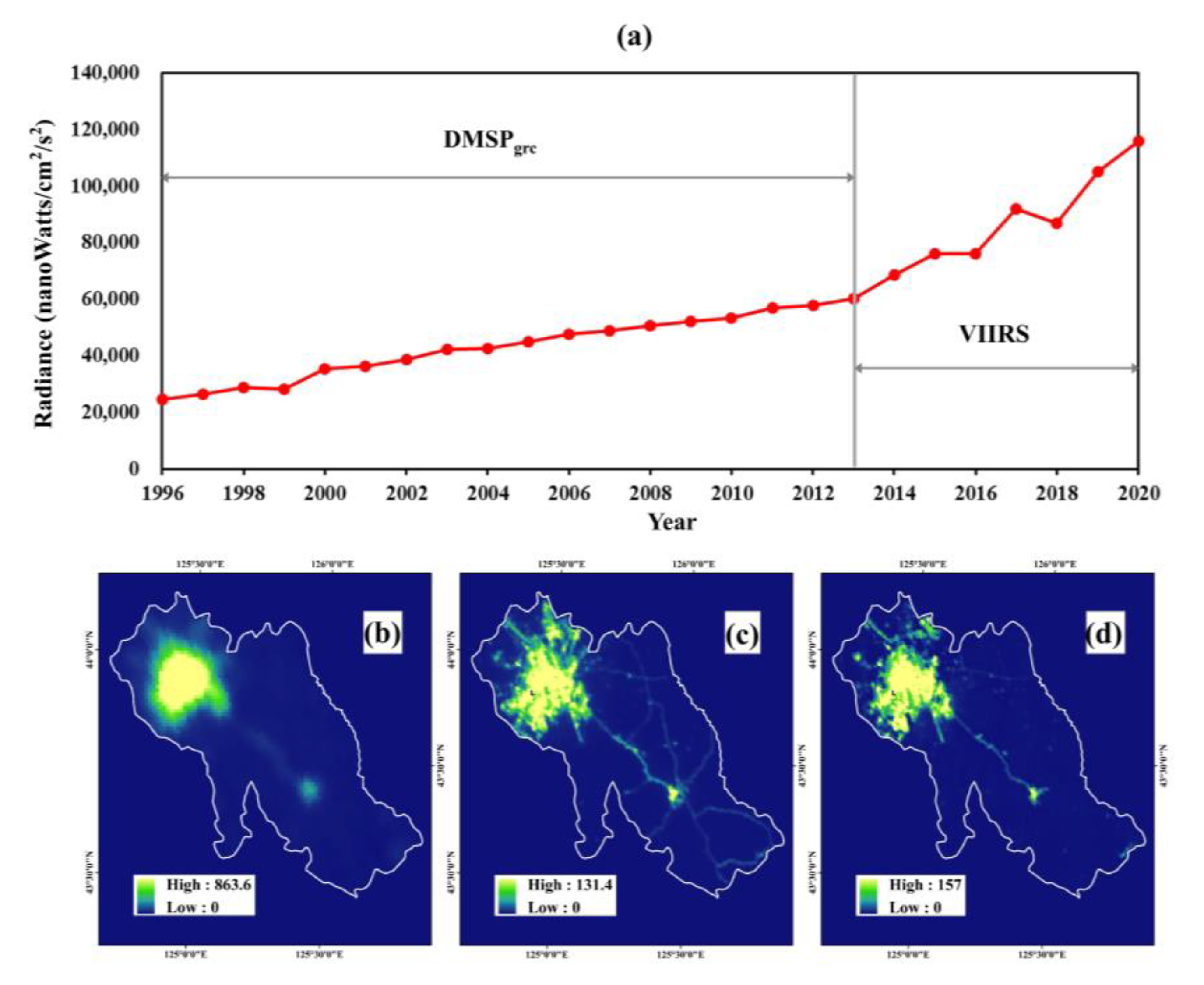
The effect of the cross-sensor calibration was checked by two aspects: the curve of the time series and the quality of the calibrated image. Figure 5, exemplified by Changchun city (the capital city of Jilin Province), illustrates the NTL time series after calibration. The NTL between the different satellite sensors is well calibrated (Figure 5a). Additionally, the calibrated DMSPgrc in Figure 5d has a better data quality than its uncalibrated counterpart (Figure 5b) in terms of a higher spatial resolution and more detailed spatial information.

Figure 5.
(a) The cross-sensor calibration results, with Changchun city, capital of Jilin Province, as an example: the total DN of calibrated time series of NTL data from 1996–2020; (b) the original DMSPgrc image in 2009; (c) the VIIRS image in 2017; and (d) the calibrated image in 2009.
For the RS results, the R2 of the model was 0.97, which met the accuracy requirement. The OOB errors of all the candidate NTL features are shown in Figure 6. Three NTL features have a normalized OOB error higher than 0.5, including the slope of the total DN, the intercept of the total DN and the slope of light pixels. Thus, they were chosen to build the NI.
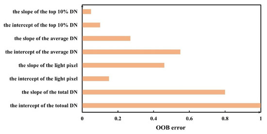
Figure 6.
The normalized OOB errors of different NTL features.
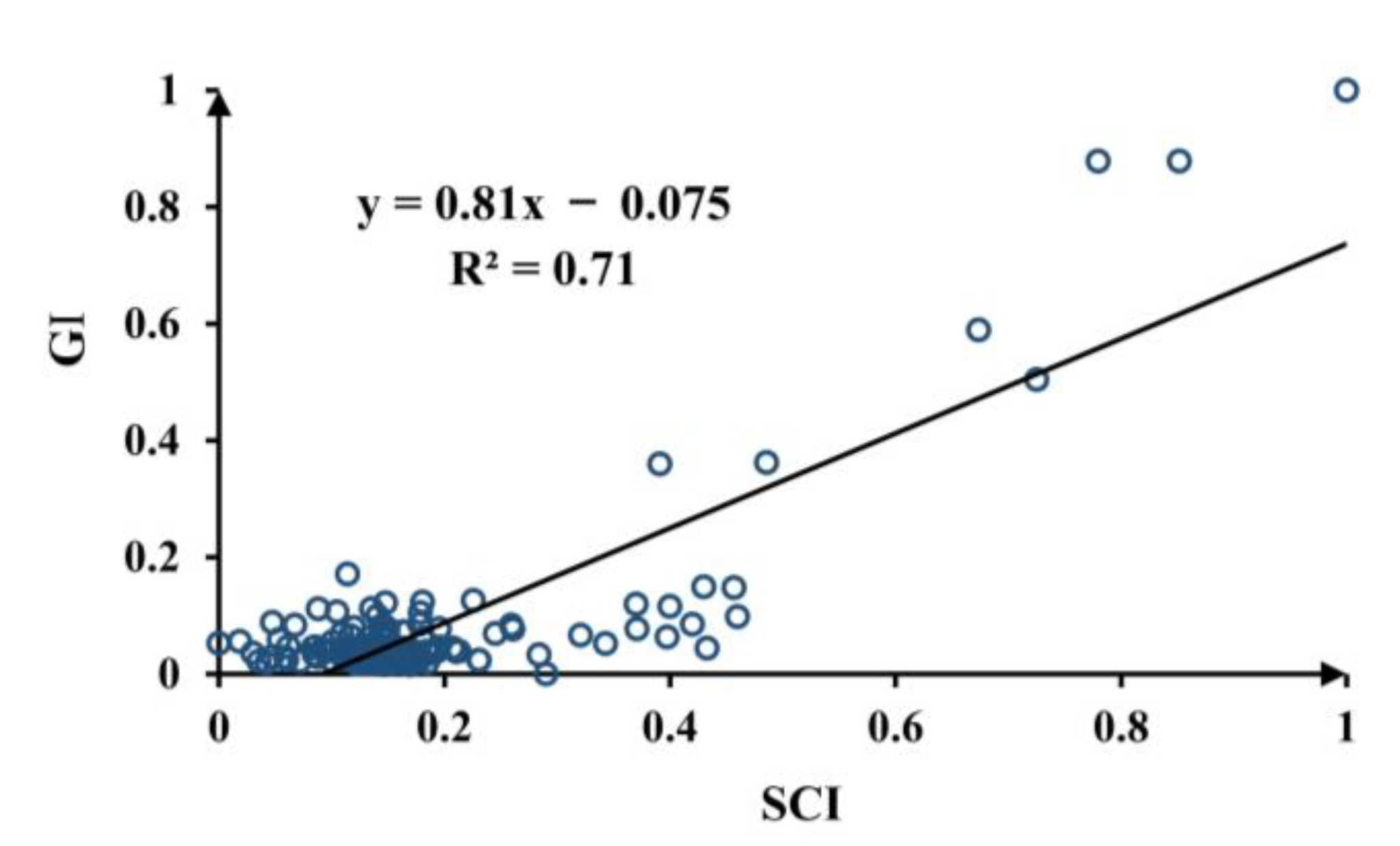
The R2 value of the linear regression model is 0.71 (Figure 7), which demonstrates that there was a certain consistency between the GI and SCI. The main deviation points are associated with cities with high GI values; this can be explained by the fact that areas where NTL was not detected may still generate economic activity during the day.
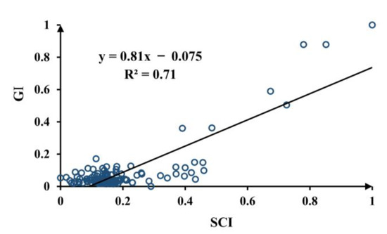
Figure 7.
Scatter plot of the GI and SCI, where the black line indicates the best fitting line.
4.2. Spatial Patterns of Shrinking Cities
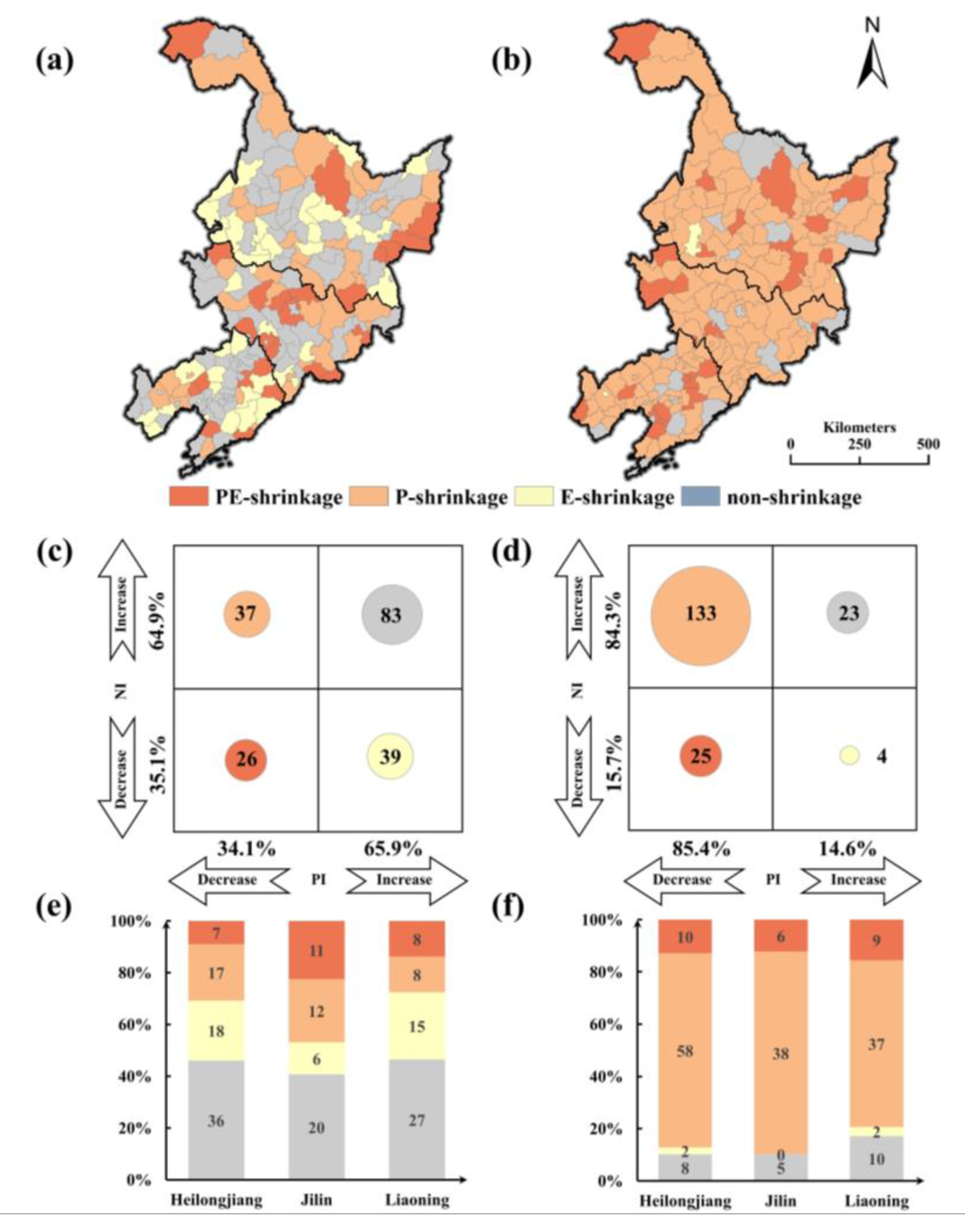
The numbers and distributions of the four types of cities were successfully identified by the proposed framework (Figure 8a,d). Overall, most of the cities have been shrinking continuously over the past 25 years. In S1, 102 shrinking cities were identified, accounting for 55.1% of the total number of cities studied. This finding indicates that city shrinkage in NEC has occurred for a long time and not just in recent years. Most of the shrinking cities were located in the northeastern and central part of NEC. The three types of shrinkage, namely, NP-shrinkage, P-shrinkage and N-shrinkage, were evenly distributed, and the numbers of the three types were 26, 37 and 39, respectively. A total of 34.1% of the cities in NEC displayed a population decline, and 35.1% of them were found to shrink according to NTL. In S2, there was a sharp increase in the number of shrinking cities, and the shrinkage pattern displayed considerable heterogeneity. Among the 185 cities, 162 cities were found to be shrinking, and only 12.4% were non-shrinking cities. A total of 133 cities were P-shrinking cities, accounting for 72% of all cities in this scenario, and only 4 cities were N-shrinking cities. The proportions of cities with decreases in population and NTL were 85.4% and 15.7%, respectively. The study results highlight a significant difference in the shrinking patterns between the two stages, suggesting that the stage division was rational to some extent.

Figure 8.
(a) The spatial distribution of different shrinkage types in S1 (1996–2009); (b) the spatial distribution of different shrinkage types in S2 (2010–2020); (c) the number of different shrinkage types in S1 (1996–2009); (d) the number of different shrinkage types in S2 (2010–2020); (e) the proportion of different shrinkage types by province in S1 (1996–2009); and (f) the proportion of different shrinkage types by province in S2 (2010–2020).
As for the shrinkage situation at the provincial level (Figure 8e,f), in S1, all three provinces had shrinking city proportions higher than 50%. Liaoning had 31 shrinking cities out of 58 total, or 53.4% of all corresponding cities, which was the lowest percentage among the three provinces. There were 7, 11 and 8 NP-shrinking cities in the three provinces, respectively. The NP-shrinking cities in Jilin accounted for 37.9% of all the shrinking cities, and this value was the highest among those for the three provinces. Eighteen N-shrinking cities and seventeen P-shrinking cities were found in Heilongjiang, more than in other provinces. In S2, NP-shrinking cities were nearly equally distributed in the three provinces. The numbers of P-shrinkage were 58, 38 and 37 in Heilongjiang, Jilin, and Liaoning, respectively, all of which accounted for large proportions of cities in these provinces; among them, Heilongjiang displayed the highest percentage. There were few N-shrinking cities in the three provinces, and there was a sharp increase in the P-shrinkage type. These results indicate that the leading cause of shrinkage in most cities in S2 was a population decrease.
Considering that the patterns of shrinkage in the two stages were quite different, we further studied the transformation situation of the four types of shrinkage from stage 1 to stage 2 (Figure 9). The largest number of type changes was found among non-shrinking cities shifting to P-shrinkage, and the number was 58, accounting for 70% of all the non-shrinkage cities in S1. The N-shrinkage category had the largest number of cities that shifted to other shrinkage types, with all the 39 cities changing to other types. Non-shrinking cities also displayed a significant transformation; 71 cities changed to other types, accounting for 85.5% of the original number. The main shift was toward P-shrinkage, with 102 cities displaying this pattern, much more than any other change type observed.
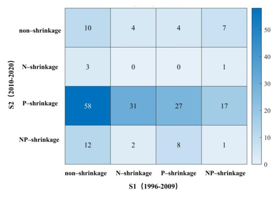
Figure 9.
Heat map of the changes for different types of shrinking cities between S1 (1996–2009) and S2 (2010–2020).
4.3. Degree of Shrinking Cities
The degree of city shrinkage in the NEC in the two periods is presented in Figure 10a,b. It is obvious that the extent of shrinkage became more severe from S1 to S2. During S1, most (77.5%) of the shrinking cities in S2 displayed medium shrinkage, and slightly and severe shrinking cities accounted for 6% and 16.7% of all cities, respectively. The severe shrinking cities were mainly located in Jilin Province. Figure 10c displays the shrinkage degree at the provincial level: the proportion of medium shrinkage was the highest in all three provinces, and that of severe shrinkage was the lowest. The intensity of city shrinkage notably increased in S2: 56 cities exhibited severe shrinkage, 71 cities exhibited medium shrinkage and only 35 cities exhibited slight shrinkage. Severely shrinking cities were mainly located in the northern part of NEC. Among the different provinces (Figure 10c,d), the shrinking degree were similar in three provinces in S1. In S2, the Liaoning Province displayed the highest proportion of non-shrinking cities, and the least proportion of severe shrinking cities among the three provinces, accounting for 13.2% and 22.4% of all the cities. The shrinking conditions in Heilongjiang Province were opposite those in Liaoning Province. Over 90% of cities were shrinking, and 38.5% were severely shrinking, the most in the three province
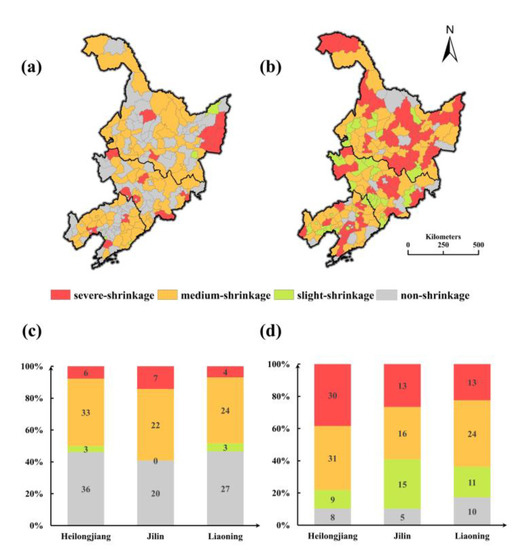
Figure 10.
(a) The degree of shrinkage in S1 (1996–2009); (b) the degree of shrinkage in S2 (2010–2020); (c) the proportions of cities with different degrees of shrinkage by province in S1 (1996–2009); and (d) the proportions of cities with different degrees of shrinkage by province in S2 (2010–2020).
5. Discussion
5.1. The Strengths and Limitations of the Proposed Method
Compared with existing methods, the merits of our proposed framework are threefold. First, consistent long-term time series of NTL data from 1996 to 2018 were constructed. The lack of long-term NTL time series is a pivotal bottleneck restricting studies of shrinking cities based on NTL data. Some recent studies have made some attempts to apply long-term time series NTL data to shrinking cities [45]. Continuous time series of data can avoid the instabilities associated with single temporal observations caused by multiple factors, and thus promote the robustness of the results. In addition, studies have shown that city shrinkage is a continuous process [23], and long-term time series provide a basis for studies of such complex and progressive issues. Most existing studies were not able to reveal the long-term trends and continuity changes related to city shrinkage due to the use of short time series [34,35]. By applying our method, the overall trend was successfully tracked, and the characteristics of city shrinkage in the early stage were detected. Moreover, the stages of city shrinkage can be divided based on consistent long-term time series. Thus, the dynamic transformations between different stages were analyzed, and the driving forces behind these shifts could be revealed. Second, to reveal the complex phenomenon of city shrinkage, NTL data and population data were integrated to establish a comprehensive indicator different from the single or basic indicators used in previous studies [34,35]. Third, our NTL index is more robust, as they were built based on representative NTL features that were extracted by the RF model.
Although this method has many advantages, there are still some aspects that can be improved. For instance, some studies pointed out that NTL data may not be a good proxy for time series measures [46,47]. We acknowledge that there are some defects in using NTL for change detection. However, we did not assert that NTL only represents economic activities, since it was regarded more as a comprehensive indicator of city shrinkage. In addition, the strength and the scope of the NTL are both important dimensions in identifying shrinking cities, and NTL is sensitive to spatial changes [48,49,50,51]. In this study, we considered both the average DN value and the light pixel area when calculating NI so that the change of spatial range and the strength variation have all been taken into consideration. We hope we can further study this topic in the future. It is reported that census data from the China City Statistical Yearbook have many problems [52]. We admit that these data have multiple defects, but they have been widely used in shrinking city studies including studies in NEC [12,13,14,53,54,55,56], and have obtained many valuable research results. Moreover, since this study is more from a long time series, large scale and macro point of view to evaluate the city shrinkage, obtaining large numbers of fine-scale confidential population data is not necessary and not feasible. Thus, we think these data are capable to be used as the auxiliary population data in this study. If more accurate or detail population grid appear in the future, we will further improve this method.
S1 and S2 were divided based on the intuitive judgement of data and the support of auxiliary information; thus, the accuracy of stage division could potentially be improved. Moreover, the division of stages was not detailed enough. We may apply more scientific methods or complex models such as time series breaking point detection method in the future study to solve these problems. When choosing the training set before applying the RF model, because a uniform standard for shrinking cities does not currently exist, we selected ten typical shrinking cities from Long’s study [12]. This caused the credibility of our results to be influenced by Long’s study. Similarly, there is currently no recognized validation dataset, which makes it difficult to verify the identification results. Previous results are not suitable for verification in this study because of the different study areas and study periods. Therefore, we merely assessed the consistency of the SCI with economic changes to verify the results to some extent. In the future, if a recognized shrinking city dataset is established, we will further verify our method by the validation dataset. In addition, we will try to find a more scientific method to verify the results by other perspectives, such as applying social media big data as validation data.
5.2. The Asynchrony of NTL and Population Changes
The most significant finding in this study is the asynchrony of NTL and population changes. This phenomenon was first observed in S1. A total of 41% of the cities in S1 were P-shrinkage or N-shrinkage cities, indicating that the changes in NI and PI were not consistent. In S2, the asynchrony of the two factors greatly increased and exhibited a significant pattern. A total of 133 cities in S2 were identified as P-shrinkage cities, accounting for 72% of all cities. These cities all experienced a decrease in population and an increase in NTL at the same time. The findings above, especially the shrinkage pattern detected in S2, are interesting. More than half of the cities in the region experienced population loss, but their NTL were still increasing. This finding contradicts intuition.
To explain these findings, the exact representation of the NTL data used in this study needs to be clarified. NTL data are normally used to reflect the intensity of human activities. Except for showing correspondence with demographic data, NTL data are highly correlated with economic activities. Several studies have used NTL data to indicate the economic activities of cities [27,37]. Since the changes in NTL data were not consistent with the changes in population data in our study, we inferred that the NI in our study possibly reflects more about the changes in city economic activities. To verify this hypothesis, we adopted linear regression for the NI with the GI and PI. The results are presented in Figure 11. The R2 value for the GI and NI is 0.67, and the R2 value for the PI and NI is 0.57. Thus, compared to population, the NI in our study has a higher correlation with economic activities. This finding suggests that focus should be placed on the scope of application when using NTL data. Some previous studies believed that population data can be directly replaced by NTL data. However, as the results of this study show, using a city shrinkage study as an example, the results based on NTL data do not always exhibit consistency with results based on population data. According to different research contents, huge differences may exist between the results derived from NTL data and population data.
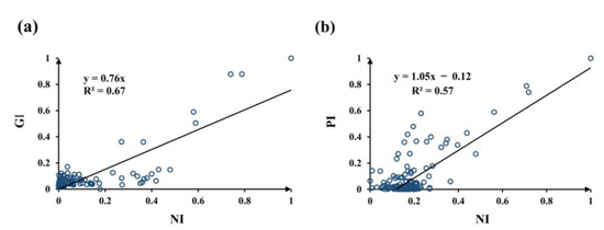
Figure 11.
(a) Scatter plot of the GI and NI, where the black line indicates the best fitting line; and (b) scatter plot of the normalized slopes of the PI and NI, where the black line indicates the best fitting line.
The uncoupling of economic activities and population growth in shrinking cities has also been noted in past studies. Bartholomae et al. [22] found that some German cities were experiencing population declines and increases in economic activities at the same time. Du et al. [10] showed that one-third of Chinese cities displayed the paradox of economic vitality growth and population decline. Shan also observed this phenomenon in the middle reaches of the Yangtze River. Our study results confirmed the existence of this phenomenon based on long-term continuous time series for the first time. Many hypotheses have been proposed by researchers to explain the cause of this phenomenon. Long et al. [12] theorized that economic decline in a shrinking city always lags behind population loss and suggested that population decline and economic growth uncoupling is a temporary phenomenon that happens in the early stage of city shrinkage. Jin et al. [57] proposed that economic development in many cities does not depend on an intensive labor force, and thus, the impact of population loss on the city economy is not very significant. Bartholomae et al. [22] proposed the concept of smart increasing; by improving the industrial structure and increasing the production capacity, city economic activities can be maintained during periods of population loss. All these theories have distinct rationality and are applicable in different situations. Additionally, these theories can be combined to explain the phenomenon observed in NEC.
According to the different causes, the P-shrinkage cities in S2 were divided into three categories, namely, economic revival cities, early-stage shrinking cities and population-insensitive cities. The detailed explanation is as follows: (1) Economic revival cities were N-shrinkage cities or NP-shrinkage cities in S1, accounting for 33.1% of all cities. The economies of these cities underwent a recovery process. Since 2005, the Chinese government began its plan to revitalize Northeast China [58], and local governments in NEC cities actively responded to the plan. The transition period from S1 to S2 coincided with the implementation period of the “Revitalization of Northeast China” policy. In this period, local governments implemented many practical measures to improve economic activities in cities. Through industrial structure transformation, these cities gradually became smartly growing cities, and their labor-intensive industries and low-efficiency industries were replaced by high-tech industries and high-efficiency industries; therefore, a reduced population could generate a sufficient production capacity and economic activities. (2) Early-stage shrinking cities were non-shrinkage cities in S1, accounting for 43.6% of all cities. Population loss began in these cities in S2; thus, these cities were in the early stages of city shrinkage. Population loss had not yet led to a further economic recession. (3) Population-insensitive cities were P-shrinkage cities in S1, accounting for 23.3% of all cities. These cities steadily experienced population loss and economic growth throughout the study period and functioned differently from other cities in the urban system. The economies in these cities do not depend on labor; thus, the effect of population loss was insignificant.
5.3. Current Situation and Policy Implications
As the results in S2 show, approximately 85% of the cities in NEC are suffering from population decline, and the annual slop change shows that this decline is accelerating. There is a high probability that the population will continue to decline in the coming years. Unlike the pessimistic population forecast, in S2, 84% of the cities in NEC showed increasing trends associated with economic activities. Thus, we can assume that the period of simultaneous declines in the economy and population in NEC is over. The population is expected to continuously decrease, and the economy is projected to continuously develop; these conditions will be the new norm for most cities in NEC.
Although the economy in some cities has recovered, the city shrinkage situation in NEC is still grim. On the one hand, the continuous loss of population is still accelerating, which may cause potential problems. On the other hand, some unreasonable policies still exist, which may worsen the shrinkage situation in NEC. The main problems are currently as follows: (1) High-quality talent may play an important role in current urban development. However, some cities in NEC only formulated policies to increase the number of residents and have ignored the proportion of high-quality talent. (2) Due to the old age of the cities in NEC, urban infrastructures are commonly poor. This issue has seriously affected the convenience of living and further reduced people’s willingness to stay. (3) Although the population has been declining for many years, some local governments consistently focused on rapid land development [59]. This unreasonable urban development strategy has further exacerbated the problem of city shrinkage. Table 2 shows the human settlement expansion rates in shrinking cities in NEC. High-speed expansion means that the land expansion rate of cities is faster than the average rate in China, while low-speed expansion means the opposite. Many NP-shrinkage cities in the two stages were also high-speed expansion cities, and this phenomenon is worthy of further assessment.

Table 2.
The human settlements expansion rate of shrinking cities in NEC.
City shrinkage is not necessarily a bad thing for urban development and management; instead, it depends on whether reasonable strategies can be adopted. In view of the city shrinkage problem in NEC, we put forward the following suggestions: (1) Change the traditional concept of urban development that focus more on quantity rather than quality is a priority for local governments, and the concept of efficient shrinkage needs to be introduced. Efficient shrinkage provides a path for solving city shrinkage problems, as noted by Popper et al. [60], who emphasized the importance of improvements in inventory, efficiency and development quality for shrinking cities. (2) Improve the management of human resources, and introduce high-tech talent. For example, Hegang has achieved great results on attracting high-tech talent through high-welfare policies, and economic activities in the city have therefore continually increased. (3) Adjust the industrial structure of traditional industrial cities, and use new technology to replace labor-intensive industries. For instance, by prohibiting new expansion of traditional industries and providing reasonable assistance to withdraw from low-efficiency, low-tech and high-energy-consumption industries, Anshan successfully reversed its shrinking trend. (4) Redefine the function of cities, and develop new plans for cites. The experience of western countries is worthy of attention in this context. In the face of continuous city shrinkage, Buffalo, NY, redefined its functional position and provided a large number of jobs. Youngstown, OH, reformulated urban planning based on small-scale urban areas and demolished built-up areas to improve the quality of urban life [60]. Because different shrinking cities have different features, practical policies should be chosen to suit their local conditions.
6. Conclusions
In this study, a novel method that combines long-term time series of NTL data and population data was applied to identify and classify shrinking cities in NEC from 1996 to 2020. In detail, we applied the GWR regression model to achieve cross-sensor calibration, and obtained long-term continuous NTL time series. Moreover, we generated NI by RF model and PI by the slope of population to indicate NTL and population change, respectively. We also combined the two indices into SCI, and identified and classified shrinking cities in NEC. The results show that most of the cities in NEC have been shrinking for the past 25 years. Moreover, the shrinkage patterns in the two stages were quite different, and economic and population changes were not synchronous. From S1 to S2, the shrinkage situation worsened, and the heterogeneity of shrinkage types increased. In S2, most of the cities experienced accelerated population decline and increases in economic activities, suggesting that governments need to maintain implementing effective measures and take the route of efficient shrinkage.
In future works, multiple sources datasets, such as industrial data, traffic data, ecological data and other types of data that are possibility related to city shrinkage, can be used to further improve the robustness of the identification of city shrinkage in this method. With multiple fine-scale auxiliary data, this method can also be improved from region scale into grid scale. In addition, this method should be further examined with other regions and cities, and establish a credible shrinking city dataset. Moreover, it is meaningful to further study the stage division of shrinking cities, more robust method should be applied to have a more detailed and accurate stage division result, and thus the driving forces of different stages can be revealed.
Author Contributions
Conceptualization, B.D.; methodology, B.D. and Y.Y.; software, B.D.; validation, B.D.; formal analysis, B.D.; investigation, B.D.; resources, B.D.; data curation, B.D.; writing—original draft preparation, B.D.; writing—review and editing, Y.Y., S.Y., Q.Z., L.H., C.Z., S.L., C.T., Y.L.; visualization, Y.Y.; supervision, B.D. and K.W. All authors have read and agreed to the published version of the manuscript.
Funding
This research was supported by the National Key Research and Development Project (2020YFC1807500), the National Natural Science Foundation of China (41971236), and the Basic Public Welfare Research Program of Zhejiang Province, China (Grant No. LGJ19D010001).
Institutional Review Board Statement
Not applicable.
Informed Consent Statement
Not applicable.
Data Availability Statement
The DMSPgrc data is collected from (https://www.ngdc.noaa.gov/eog/dmsp/download_radcal.html) (accessed on 15 August 2020). The NPP-VIIRS is downloaded from (Index of/nighttime_light/annual/v20 (mines.edu)) (accessed on 12 June 2021). The population and GDP census data can be found in (http://www.stats.gov.cn/ztjc/ztsj/hstjnj/) (accessed on 17 August 2020). The human settlement data can be found in (http://data.ess.tsinghua.edu.cn) (accessed on 28 September 2020). All the data above are open access.
Acknowledgments
We would like to thank reviewers and the editor for their constructive comments and suggestions. This research was supported by the National Key Research and Development Project (2020YFC1807500), the National Natural Science Foundation of China (41971236), and the Basic Public Welfare Research Program of Zhejiang Province, China (Grant No. LGJ19D010001).
Conflicts of Interest
The authors declare no conflict of interest.
References
- Häußermann, H.; Siebel, W. Die Schrumpfende Stadt und Die Stadtsoziologie; Westdeutscher V Erlag: Opladen, Germany, 1988; pp. 78–94. [Google Scholar]
- Wiechmann, T.; Pallagst, K.M. Urban shrinkage in Germany and the USA: A Comparison of Transformation Patterns and Local Strategies. Int. J. Urban Reg. Res. 2012, 36, 261–280. [Google Scholar] [CrossRef]
- Haase, A.; Nelle, A.; Mallach, A. Representing urban shrinkage—The importance of discourse as a frame for understanding conditions and policy. Cities 2017, 69, 95–101. [Google Scholar] [CrossRef]
- Danko, J.J.; Hanink, D.M. Beyond the obvious: A comparison of some demographic changes across selected shrinking and growing cities in the United States from 1990 to 2010. Popul. Space Place 2018, 24, e2136. [Google Scholar] [CrossRef]
- Hattori, K.; Kaido, K.; Matsuyuki, M. The development of urban shrinkage discourse and policy response in Japan. Cities 2017, 69, 124–132. [Google Scholar] [CrossRef]
- Mallach, A. What we talk about when we talk about shrinking cities: The ambiguity of discourse and policy response in the United States. Cities 2017, 69, 109–115. [Google Scholar] [CrossRef]
- Wolff, M.; Wiechmann, T. Urban growth and 3ecline: Europe’s shrinking cities in a comparative perspective 1990–2010. Eur. Urban Reg. Stud. 2018, 25, 122–139. [Google Scholar] [CrossRef]
- Pallagst, K. From urban shrinkage to urban qualities? J. Urban Des. 2019, 24, 68–70. [Google Scholar] [CrossRef]
- Martinez-Fernandez, C.; Weyman, T.; Fol, S.; Audirac, I.; Cunningham-Sabot, E.; Wiechmann, T.; Yahagi, H. Shrinking cities in Australia, Japan, Europe and the USA: From a global process to local policy responses. Prog. Plan. 2016, 105, 1–48. [Google Scholar] [CrossRef]
- Du, Z.; Li, X. Characteristic and mechanism of urban growth and shrinkage from demographic change perspective: A case study of Dongguan. Sci. Geogr. Sin. 2018, 6, 1837–1846. [Google Scholar]
- Du, Z.; Li, X. Growth or shrinkage: New phenomena of regional development in the rapidly-urbanising Pearl River Delta. Acta Geogr. Sin. 2017, 10, 1800–1811. [Google Scholar]
- Long, Y.; Wu, K. Shrinking cities in a rapidly urbanizing China. Environ. Plann. A 2016, 2, 220–222. [Google Scholar] [CrossRef] [Green Version]
- Liu, F.; Zhu, X.; Chen, J.; Sun, J.; Lin, X. The research on the quantitative identification and cause analysis of urban shrinkage from different dimensions and scales: A case study of northeast China during transformation period. Mod. City Res. 2018, 7, 37–46. [Google Scholar]
- Ma, Z.; Li, C.; Zhang, J. Understanding Urban Shrinkage from a Regional Perspective: Case Study of Northeast China. J. Urban Plan. Dev. 2020, 146, 04020027. [Google Scholar] [CrossRef]
- Richardson, H.W.; Nam, C.W. Shrinking Cities: A Global Perspective; Routledge: London, UK, 2014. [Google Scholar]
- Bernt, M. The Limits of Shrinkage: Conceptual Pitfalls and Alternatives in the Discussion of Urban Population Loss. Int. J. Urban Reg. Res. 2016, 40, 441–450. [Google Scholar] [CrossRef]
- Dubeaux, S.; Cunningham Sabot, E. Maximizing the potential of vacant spaces within shrinking cities, a German approach. Cities 2018, 75, 6–11. [Google Scholar] [CrossRef]
- Audirac, I. Introduction: Shrinking Cities from marginal to mainstream: Views from North America and Europe. Cities 2018, 75, 1–5. [Google Scholar] [CrossRef]
- Reis, J.P.; Silva, E.A.; Pinho, P. Spatial metrics to study urban patterns in growing and shrinking cities. Urban Geogr. 2016, 37, 246–271. [Google Scholar] [CrossRef]
- Oswalt, P.; Rieniets, T. Atlas of Shrinking Cities; Hatje Cantz: Ostfildern, Germany, 2006. [Google Scholar]
- Schilling, J.; Logan, J. Greening the rust belt: A green infrastructure model for right sizing America’s shrinking cities. J. Am. Plan. 2008, 4, 451–466. [Google Scholar] [CrossRef]
- Bartholomae, F.; Woon Nam, C.; Schoenberg, A. Urban shrinkage and resurgence in Germany. Urban Stud. 2017, 54, 2701–2718. [Google Scholar] [CrossRef]
- Alves, D.; Barreira, A.P.; Guimarães, M.H.; Panagopoulos, T. Historical trajectories of currently shrinking Portuguese cities: A typology of urban shrinkage. Cities 2016, 52, 20–29. [Google Scholar] [CrossRef] [Green Version]
- He, S.Y.; Lee, J.; Zhou, T.; Wu, D. Shrinking cities and resource-based economy: The economic restructuring in China’s mining cities. Cities 2017, 60, 75–83. [Google Scholar] [CrossRef]
- Khavarian-Garmsir, A.R.; Pourahmad, A.; Hataminejad, H.; Farhoodi, R. Climate change and environmental degradation and the drivers of migration in the context of shrinking cities: A case study of Khuzestan province, Iran. Sustain. Cities Soc. 2019, 47, 101480. [Google Scholar] [CrossRef]
- Döringer, S.; Uchiyama, Y.; Penker, M.; Kohsaka, R. A meta-analysis of shrinking cities in Europe and Japan. Towards an integrative research agenda. Eur. Plan. Stud. 2020, 28, 1693–1712. [Google Scholar] [CrossRef] [Green Version]
- Shan, J.; Liu, Y.; Kong, X.; Liu, Y.; Wang, Y. Identifying City Shrinkage in Population and City Activity in the Middle Reaches of the Yangtze River, China. J. Urban Plan. Dev. 2020, 146, 05020025. [Google Scholar] [CrossRef]
- Olsen, A.K. Shrinking Cities: Fuzzy Concept or Useful Framework? Berkeley Plann. J. 2013, 26, 107–132. [Google Scholar] [CrossRef] [Green Version]
- Shi, K.; Yu, B.; Huang, Y.; Hu, Y.; Yin, B.; Chen, Z.; Chen, L.; Wu, J. Evaluating the Ability of NPP-VIIRS Nighttime Light Data to Estimate the Gross Domestic Product and the Electric Power Consumption of China at Multiple Scales: A Comparison with DMSP-OLS Data. Remote Sens. 2014, 6, 1705–1724. [Google Scholar] [CrossRef] [Green Version]
- Shi, K.; Chen, Y.; Yu, B.; Xu, T.; Yang, C.; Li, L.; Huang, C.; Chen, Z.; Liu, R.; Wu, J. Detecting spatiotemporal dynamics of global electric power consumption using DMSP-OLS nighttime stable light data. Appl. Energy 2016, 184, 450–463. [Google Scholar] [CrossRef]
- Bagan, H.; Borjigin, H.; Yamagata, Y. Assessing nighttime lights for mapping the urban areas of 50 cities across the globe. Environ. Plan. B Urban Anal. City Sci. 2018, 46, 1097–1114. [Google Scholar] [CrossRef]
- Wang, Y.; Huang, C.; Zhao, M.; Hou, J.; Zhang, Y.; Gu, J. Mapping the Population Density in Mainland China Using NPP/VIIRS and Points-Of-Interest Data Based on a Random Forests Model. Remote Sens. 2020, 12, 3645. [Google Scholar] [CrossRef]
- Elvidge, C.; Baugh, K.; Zhizhin, M.; Hsu, F.C.; Ghosh, T. VIIRS night-time lights. Int. J. Remote Sens. 2017, 21, 5860–5879. [Google Scholar] [CrossRef]
- Niu, W.; Xia, H.; Wang, R.; Pan, L.; Meng, Q.; Qin, Y.; Li, R.; Zhao, X.; Bian, X.; Zhao, W. Research on Large-Scale Urban Shrinkage and Expansion in the Yellow River Affected Area Using Night Light Data. ISPRS Int. J. Geo-Inf. 2021, 10, 5. [Google Scholar] [CrossRef]
- Jiang, Z.; Zhai, W.; Meng, X.; Long, Y. Identifying Shrinking Cities with NPP-VIIRS Nightlight Data in China. J. Urban Plan. Dev. 2020, 146, 04020034-1. [Google Scholar] [CrossRef]
- Zhou, Y.; Li, C.; Ma, Z.; Hu, S.; Zhang, J.; Liu, W. Identification of Shrinkage and Growth Patterns of a Shrinking City in China Based on Nighttime Light Data: A Case Study of Yichun. Sustainability 2019, 11, 6906. [Google Scholar] [CrossRef] [Green Version]
- Lang, W.; Deng, J.; Li, X. Identification of “Growth” and “Shrinkage” Pattern and Planning Strategies for Shrinking Cities Based on a Spatial Perspective of the Pearl River Delta Region. J. Urban Plan. Dev. 2020, 146, 05020020. [Google Scholar] [CrossRef]
- Zheng, Q.; Weng, Q.; Wang, K. Developing a new cross-sensor calibration model for DMSP-OLS and Suomi-NPP VIIRS night-light imageries. ISPRS J. Photogramm. 2019, 153, 36–47. [Google Scholar] [CrossRef]
- China Statistical Yearbook; China State Statistics Bureau: Beijing, China, 2012.
- China Statistical Yearbook; China State Statistics Bureau: Beijing, China, 2017.
- Elvidge, C.; Zhizhin, M.; Ghosh, T.; Hsu, F.C. Annual Time Series of Global VIIRS Nighttime Lights Derived from Monthly Averages: 2012 to 2019. Remote Sens. 2021, 13, 922. [Google Scholar] [CrossRef]
- Gong, P.; Li, X.; Zhang, W. 40-Year (1978–2017) human settlement changes in China reflected by impervious surfaces from satellite remote sensing. Sci. Bull. 2019, 64, 756–763. [Google Scholar] [CrossRef] [Green Version]
- Brunsdon, C.; Fotheringham, A.S.; Charlton, M.E. Geographically weighted regression: A method for exploring spatial nonstationarity. Geogr. Anal. 1996, 28, 281–298. [Google Scholar] [CrossRef]
- Breiman, L. Random Forests. Mach. Learn. 2001, 45, 5–32. [Google Scholar] [CrossRef] [Green Version]
- Yang, Y.; Jianguo, W.; Ying, W.; Qingxu, H.; Chunyang, H. Quantifying spatiotemporal patterns of shrinking cities in urbanizing China: A novel approach based on time-series nighttime light data. Cities 2021, 118, 103346. [Google Scholar] [CrossRef]
- Xi, C.; William, N. VIIRS Nighttime Lights in the Estimation of Cross-Sectional and Time-Series GDP. Remote Sens. 2019, 11, 1057. [Google Scholar]
- William, N.; Xi, C. A sharper image? Estimates of the precision of nighttime lights as a proxy for economic statistics. J. Econ. Geogr. 2015, 15, 217–246. [Google Scholar]
- Sun, J.; Di, L.; Sun, Z.; Wang, J.; Wu, Y. Estimation of GDP Using Deep Learning With NPP-VIIRS Imagery and Land Cover Data at the County Level in CONUS. IEEE J. Sel. Top. Appl. Earth Obs. Remote. Sens. 2020, 13, 1400–1415. [Google Scholar] [CrossRef]
- Xie, Y.; Weng, Q. Detecting urban-scale dynamics of electricity consumption at Chinese cities using time-series DMSP-OLS (Defense Meteorological Satellite Program-Operational Linescan System) nighttime light imageries. Energy 2016, 100, 177–189. [Google Scholar] [CrossRef]
- Zhao, M.; Zhou, Y.; Li, X.; Cheng, W.; Zhou, C.; Ma, T.; Li, M.; Huang, K. Mapping urban dynamics (1992–2018) in Southeast Asia using consistent nighttime light data from DMSP and VIIRS. Remote Sens. Environ. 2020, 248, 111980. [Google Scholar] [CrossRef]
- Zhao, N.; Liu, Y.; Hsu, F.; Samson, E.L.; Letu, H.; Liang, D.; Cao, G. Time series analysis of VIIRS-DNB nighttime lights imagery for change detection in urban areas: A case study of devastation in Puerto Rico from hurricanes Irma and Maria. Appl. Geogr. 2020, 120, 102222. [Google Scholar] [CrossRef]
- Gibson, J.; Li, C. The Erroneous use of China’s Population and per Capita Data: A Structured Review and Critical Test. J. Econ. Surv. 2017, 31, 905–922. [Google Scholar] [CrossRef]
- Guan, D.; He, X.; Hu, X. Quantitative identification and evolution trend simulation of shrinking cities at the county scale, China. Sustain. Cities Soc. 2021, 65, 102611. [Google Scholar] [CrossRef]
- Yan, G.; Chen, X.; Zhang, Y. Shrinking cities distribution pattern and influencing factors in Northeast China based on random forest model. Sci. Geogr. Sin. 2021, 41, 880–889. [Google Scholar]
- Ma, Z.; Li, C.; Zhang, J. Characteristics, mechanism and response of urban contraction in Northeast China. Acta Geogr. Sin. 2021, 76, 767–780. [Google Scholar]
- Tong, Y.; Liu, W.; Li, C. Understanding patterns and multilevel influencing factors of small town shrinkage in Northeast China. Sustain. Cities Soc. 2021, 68, 102811. [Google Scholar] [CrossRef]
- Jin, L. Research on the inter-influences between hidden shrinkage of urban population and economic growth—A case study of Maoming in Guangdong Province. J. Harbin Inst. 2018, 1, 133–140. [Google Scholar]
- Sun, J.; Su, X. The strategy of urban smart growth in vied of the revitalization of Northeast China. Soc. Sci. J. 2020, 5, 50–62. [Google Scholar]
- Zheng, Q.; Deng, J.; Jiang, R.; Wang, K.; Xue, X.; Lin, Y.; Huang, Z.; Shen, Z.; Li, J.; Shahtahmassebi, A.R. Monitoring and assessing “ghost cities” in Northeast China from the view of nighttime light remote sensing data. Habitat Int. 2017, 70, 34–42. [Google Scholar] [CrossRef]
- Popper, D.E.; Popper, F.J. Small Can be Beautiful:Coming to Terms with Decline. Planning 2002, 7, 20–23. [Google Scholar]
Publisher’s Note: MDPI stays neutral with regard to jurisdictional claims in published maps and institutional affiliations. |
© 2021 by the authors. Licensee MDPI, Basel, Switzerland. This article is an open access article distributed under the terms and conditions of the Creative Commons Attribution (CC BY) license (https://creativecommons.org/licenses/by/4.0/).


