Abstract
Small mammals, and particularly rodents, are common inhabitants of farmlands, where they play key roles in the ecosystem, but when overabundant, they can be major pests, able to reduce crop production and farmers’ incomes, with tangible effects on the achievement of Sustainable Development Goals no 2 (SDG2, Zero Hunger) of the United Nations. Farmers do not currently have a standardized, accurate method of detecting the presence, abundance, and locations of rodents in their fields, and hence do not have environmentally efficient methods of rodent control able to promote sustainable agriculture oriented to reduce the environmental impacts of cultivation. New developments in unmanned aerial system (UAS) platforms and sensor technology facilitate cost-effective data collection through simultaneous multimodal data collection approaches at very high spatial resolutions in environmental and agricultural contexts. Object detection from remote-sensing images has been an active research topic over the last decade. With recent increases in computational resources and data availability, deep learning-based object detection methods are beginning to play an important role in advancing remote-sensing commercial and scientific applications. However, the performance of current detectors on various UAS-based datasets, including multimodal spatial and physical datasets, remains limited in terms of small object detection. In particular, the ability to quickly detect small objects from a large observed scene (at field scale) is still an open question. In this paper, we compare the efficiencies of applying one- and two-stage detector models to a single UAS-based image and a processed (via Pix4D mapper photogrammetric program) UAS-based orthophoto product to detect rodent burrows, for agriculture/environmental applications as to support farmer activities in the achievements of SDG2. Our results indicate that the use of multimodal data from low-cost UASs within a self-training YOLOv3 model can provide relatively accurate and robust detection for small objects (mAP of 0.86 and an F1-score of 93.39%), and can deliver valuable insights for field management with high spatial precision able to reduce the environmental costs of crop production in the direction of precision agriculture management.
1. Introduction
Sustainable agriculture and farm resilience are the main objectives of this century. United Nations and FAO, through Sustainable Development Goal 2 (SDG2—Zero Hunger) and the Sustainable Crop Production Intensification (SCPI) Strategic Objective A of FAO Strategic Framework 2010–2019 [1], underline the need to achieve food security under climate change through the improvement of farm resource use efficiency and at the same time reducing the environmental impacts (e.g., plant biotic stress control).
In many productive agricultural contexts, small mammals, and particularly rodents are common inhabitants of farmlands playing key roles in the ecosystem. However, when overabundant they behave as pests, able to reduce crop production and farmers’ incomes and requiring the phytosanitary treatments of the field which are environmental and farmer costs [2,3]. Then an environmentally efficient method of rodent control able to promote sustainable agriculture, reducing the number and entity of treatments, oriented to reduce the environmental impacts of cultivation is not present.
Currently, no studies have been found to indicate a reference methodology to detect the presence, abundance, and location of small rodent holes in the field. To address this, the ability to detect small objects via optical remote sensing and deep learning approaches, using very high-resolution imagery from unmanned aircraft systems (UASs) can be helpful [4], but the problem of backgrounds complexity of field images to estimate the exact position, localization, and classification of an object must be faced and overcome.
Before the development of deep learning approaches, conventional object detection schemes for remote-sensing applications (based on handcrafted features and shallow machine learning models) were based on three main steps: (i) selecting the regions of interest (ROIs) in which objects may appear; (ii) extracting the local characteristics; and (iii) applying a supervised classifier to these features [5]. The main drawback was the limited robustness due to restrictions on the representation of various backgrounds in a given set of data, which created overfitting and required many calculations [6]. The emerging development of deep neural networks, and specifically convolutional neural networks (CNNs), brought a substantial paradigm change and significant improvements in the generalization and robustness of automatic learning and extraction using features from annotated training data [5,7]. In many recent applications, traditional object detection models have been replaced by deep learning-based models, which are considered to be more accurate [8].
The region-based CNN (R-CNN), proposed in 2014, was a major milestone in object detection [9] together with other bounding box regression-based approaches such as Fast R-CNN [10], Faster R-CNN [11], and R-FCN (region-based fully convolutional network) [12]. These image segmentation methods produce a relatively low detection rate in natural settings [13,14]. To ensure good results, deep learning approaches need to include both detection and classification stages. For example, Faster R-CNN uses a region proposal network (RPN) method to classify bounding boxes, and fine-tuning is then applied to process these bounding boxes [15,16]. An alternative approach is a one-pass regression based on class probabilities and bounding box locations, as used in the single-shot multibox detector (SSD) [17], deeply supervised object detector (DSOD) [18], RetinaNet [19], EfficientDet [20], You Only Look Once (YOLO) [21,22], etc. These methods unite target classification and localization into a regression analysis, do not require RPN, and directly perform regression to detect targets in the image.
The success rate of CNN-based object detection methods is dependent on the network architecture and the quality and annotation of the data. In terms of feature maps, most deep high-level maps have low resolution, thus making the detection of small objects a challenging task. Both one-stage and two-stage detector models have certain disadvantages: one-stage models are less detailed, and therefore have difficulty detecting small objects, whereas two-stage models have long process times. In comparison, the use of low-resolution feature maps (coarse, deep features) can reduce the performance of high-quality localization models due to the loss of detailed information and the long processing times for two-stage models. Shallow, low-level feature maps can reduce the representative capacity for recognition and classification. One possible alternative is an attention-based model, which can effectively extract the features of objects and enhance the detection performance through a complementary combination of both low- and high-level features [23].
Over the past decade, one- and two-stage models have been used for object detection using aerial, UAS, and satellite remote-sensing images [24]. However, computer vision models cannot be directly transferred to remote-sensing applications, in particular, due to the geospatial properties of the objects that appear in the scenes. As previously reported [25], the objects of interest in remote-sensing data are heterogeneous in terms of their size and shape and cover a wide range of spectral signatures depending on the sensor, scanning geometry, lighting, weather conditions, etc. Furthermore, compared with natural images (in which the focus is on the central foreground object of interest, the background is blurred, and images are collected at close range), remote-sensing images in general and UAS-based images, in particular, involve small objects (scanned from above from a given flight altitude) and complex backgrounds (where the surface of the ground around the object of interest does not have a specific focus or blurriness, and there is no prior identified or preferable foreground). Since the feature maps obtained by CNNs have gradually been reduced over time due to the use of convolution and down-sampling operations, the present study aims to investigate the accurate, detailed detection of small objects in UAS-based remote-sensing images. The main objective of the study is to compare the performance of selected one- and two-stage detector models on a single UAS-based image and a processed (via Pix4D mapper photogrammetric program) UAS-based orthophoto product for agriculture/environmental applications. We then assess and report on the use of a multimodal dataset for small object detection.
2. Motivation
The 2030 SDG deadline is just a decade away, and the Commitments of SDG2 include taking action to fight hunger and malnutrition and supporting sustainable agriculture, including forestry, fisheries, and pastoralism. The agenda pledges to strengthen efforts to enhance food security and nutrition. Therefore, it is impossible to skip the issue of the modern agricultural landscapes that transformed natural habitats into large mosaics of monoculture, containing scattered uncultivated regions of semi-natural habitats with varying dimensions and shapes. This variety of agricultural environments has resulted in a loss of habitat heterogeneity that affects biodiversity and ecosystem function [26]. Rodents such as Microtus voles play a keystone functional role within ecological communities, as they are the main food source for a variety of predators, and are also a major agricultural pest in terms of damage to field crops, stored grain, and farm equipment each year [27,28]. For example, in Israel, populations of Levant voles (Microtus guentheri) can create thousands of burrow openings per hectare [29] as a result of the voles’ very high reproductive output. Levant voles reach reproductive age within the first month of being born, pregnancy lasts only 21 days, and they raise five or six young per litter [30,31]. Vole populations can therefore fluctuate rapidly, causing extensive agricultural loss [32].
To combat the problem of voles, farmers have used rodenticides. For example, in the United States, approximately 30 million pounds of rodenticides and other conventional pesticides are used in agricultural, suburban, and urban settings each year [33]. Although rodent baits placed in agricultural settings can kill rodents very effectively [27], they pose a potential threat to non-target wildlife through secondary poisoning [34] and there are also fears of resistance [35,36]. The cost of controlling voles is high, not only due to the damage caused but because rodenticides are expensive (in terms of the cost of purchasing and distribution in the field).
Although integrated pest control methods for controlling voles have been suggested that combine irrigation to flood fields and the introduction of natural predators [37,38], these methods have not solved the problem completely, and rodenticide is still used. One of the major problems with controlling voles is that farmers do not have methods for determining the abundance and locations of voles in their fields. In general, farmers only start to notice voles when the population is large since damage from voles creates “bald” sections in the field that are visible. Farmers traditionally apply large amounts of rodenticide as a form of prevention, before they even see the voles, and add even larger quantities when they see the damage. There is, therefore, a need to develop a method of determining the locations of the voles in a field when the population numbers are small; this would allow farmers to control only certain specific areas, therefore increasing the efficiency of control and reducing the amounts of rodenticide required.
Precision agriculture (PA) is a method of managing crop fields that takes into consideration spatial variation and local field requirements. PA involves data collection to characterize the spatial variability of fields, mapping, decision making, and the implementation of management practices [39]. The development of UAS-borne remote-sensing imagery has increased the number of precision agriculture applications, due to the ability of UASs to carry out cost-effective, low-altitude flights in small fields and to produce images with high spatial (i.e., centimeter) and temporal (i.e., daily) resolutions [40]. The main motivation for the present study is to provide a framework for the precise detection of vole holes that applies sensor, platform, and advanced data processing approaches based on machine learning algorithms to monitor and analyze the vole population in an agricultural setting. The study is carried out at the landscape scale, and focuses on detector accuracy as a function of habitat composition (abundance of burrow systems), structural landscape heterogeneity (e.g., crop or soil background), and the influence of UAS imagery by comparing the performance of deep object detection models on an orthophoto product versus individual/single UAS images. The following deep learning-based algorithms are evaluated in this paper: Faster R-CNN, YOLOv3, YOLOv5, EfficientNet, and RetinaNet. For each method, a detailed description of the model architecture, the parameter settings used for training, and any additional stages such as pre-processing, multimodal data, and post-processing, are provided.
3. Materials and Methods
3.1. Object Detection Models
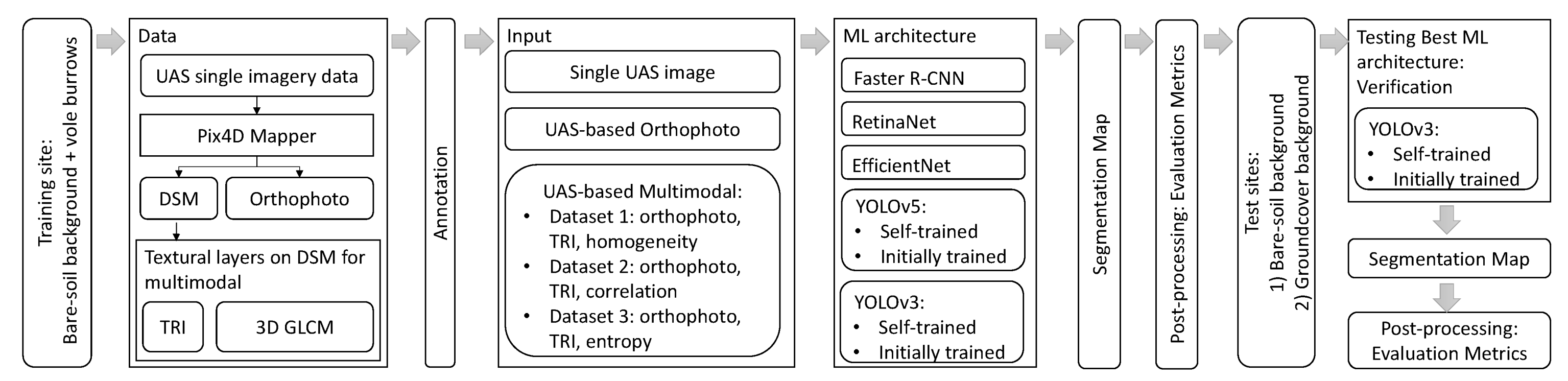
This section presents a comprehensive description of the object detection methods used: Faster R-CNN, YOLOv3, YOLOv5, and EfficientNet and RetinaNet, in the general flowchart of the study (Figure 1).
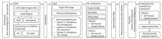
Figure 1.
Overall flowchart.
Faster R-CNN [41] is a two-stage object detection model that generates a sparse set of entrant objects using a region pooling network (RPN) based on feature maps and classifies each object as foreground or background. After extracting the feature maps with a CNN, a set of bounding boxes at the object locations is generated in the first stage via an RPN. The size of each anchor is configured using hyperparameters. The region of interest pooling layer (RoI pooling) generates sub-feature maps that are converted into dimensional vectors and fed forward to fully connected layers. These layers are then used as a regression network to predict the bounding box offsets, and a classification network is applied to predict the class label for each bounding box. The attention network is used to avoid misalignments between the RoI and the extracted features of the RoIAlign layer (introduced in Mask R-CNN [41]). In this study, Faster R-CNN with a RoIAlign layer is applied within ResNeXt101 [42], with a feature pyramid network (FPN) [43] feature extraction backbone. FPN provides lateral connections that can enhance the semantic characteristics of shallow layers via a top-down pathway that promotes generic feature extraction.
The YOLO family of models [21] are end-to-end deep learning-based detection models that determine the bounding boxes of the objects present in the image and classify them in a single pass. This approach does not involve region proposal steps, unlike two-stage detectors. The YOLO network first splits the input image into a grid of non-overlapping cells and predicts three elements for each cell: (i) the probability of an object being present; (ii) the coordinates of the box surrounding it (only if there is an object in this cell); and (iii) the class to which the object belongs and the associated probability. YOLO is an anchor-free algorithm and performs regression of the target position and category for each pixel of the feature map. The development of YOLOv3 [22] improved the detection accuracy, and in particular allowed the model to find objects of different sizes, as it offered three detection levels rather than only one in the previous versions, thus supporting the detection of smaller objects. YOLOv3 predicts three-box anchors for each cell, detects at three different levels with the searching grids, and exploits a deeper backbone network (Darknet-53) for feature map extraction. However, since YOLOv3 offers a deeper feature extraction network with three-level prediction, it is also slower, as one-stage detectors are generally characterized by rather lower accuracy in terms of detecting small objects from remote-sensing images [44]. As the detection algorithm is required to detect only one type of object, the complexity of the problem is reduced when only a single object is under investigation. YOLOv5 is a high-precision, real-time detection network with a cross-stage partial network (CSPNet) Darknet [45] feature extraction backbone, which reduces the number of model parameters, thus not only ensuring the speed and accuracy of inference but also reducing the size of the model.
YOLOv5 includes four models: the smallest is YOLOv5s, with 7.5 million parameters (plain 7 MB, COCO pre-trained 14 MB) and 140 layers, and the largest is YOLOv5x, with 89 million parameters and 284 layers (plain 85 MB, COCO pre-trained 170 MB). In the approach proposed in this study, a pre-trained YOLOv5x model is used. This model includes a two-stage detector consisting of a CSPNet [45] backbone trained on MS-COCO [20], and a model head using a path aggregation network (PANet) [46] for instance segmentation. Each bottleneck unit consists of two convolutional layers with 1 × 1 and 3 × 3 filters. The backbone incorporates a spatial pyramid pooling network (SSP) [47], which allows for dynamically sized input images and is robust against object deformations.
EfficientNet is an anchor-based [20], efficient target detection algorithm. It consists of three parts: (i) a pre-trained backbone network based on ImageNet; (ii) BiFPN, which creates top-down and bottom-up feature fusion by adopting a weighted feature fusion scheme to obtain semantic information of different sizes in the model; and (iii) a classification and detection box prediction network. Feature extraction in EfficientNet-B3 is based on the idea that a small number of feature map parameters should provide rich information, thus ensuring fast, accurate detection.
The RetinaNet model consists of three parts: (i) a residual network (ResNet) [42], which is used to extract image features; (ii) an FPN for feature processing; and (iii) a classification and return sub-network, which is used to output the final detection. The number of layers is directly proportional to the abstraction degree of feature extraction and adjustable parameters, where the higher the number, the better the fitting effect. Since ResNet’s residual unit structure adds a connection to the convolution feedforward network, a deeper neural network can be trained. After the image has been passed through the deep ResNet, the features are first extracted and then fused by the FPN, and finally sent to the classification and return sub-network.
3.2. Field Study
In this section, we present the details of the dataset used in this field study and then describe the setup and the standard evaluation metrics.
3.2.1. Dataset
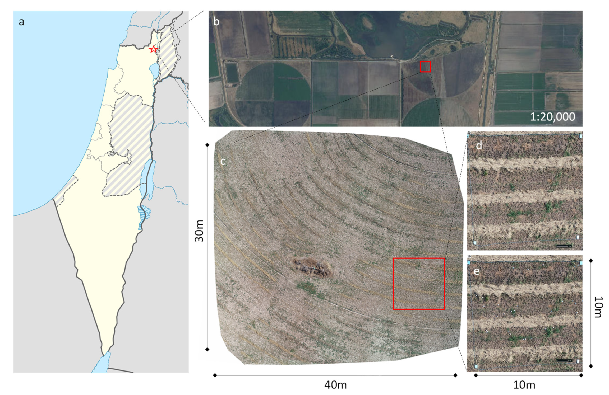
Research area: This study took place in an alfalfa (Medicago sativa) field (~25 acres) located in the Hula Valley in Israel (33.14868 N, 35.60398 E) in (Figure 2). Alfalfa is a perennial plant variety that is mainly used for animal feed (e.g., for dairy cows, horses, and sheep), and is grown for 2–6 years. During this time, the alfalfa is trimmed/harvested monthly between April and October, but because the fields are not plowed, the burrows of Levant voles are not destroyed, allowing the numbers of rodents and visible burrows to increase. Alfalfa was selected as a crop due to many voles and burrows. In this study, the burrows were counted regardless its status (active or inactive).
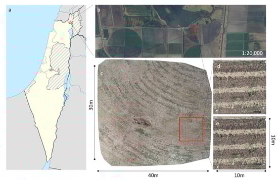
Figure 2.
Field study area, (a) the general location; (b) aerial orthophotograph (photographic scale 1:20,000) of the Alfalfa fields (national database delivered by Ofek Aerial Photography LTD published on www.govmap.gov.il, accessed on 17 July 2021); (c) UAS-based orthophoto map of a selected area (30 × 40 m); (d) a selected plot area marked by four rectangle ground targets in the corners; (e) the same plot as in c after marking burrows with white Styrofoam balls.
UAS platform and data collection—A DJI Phantom 4 Pro platform equipped with an inbuilt three-axis gimbal-stabilized 20-megapixel camera was used for RGB image acquisition. Pix4Dcapture software (Pix4D, Lausanne, Switzerland) was used to control the flight and to capture the RGB images using pre-programmed flight plans applying a frontal overlap of 90% and an adjusted side overlap (by an amount of flight). The image sequences were collected in Pix4Dcapture software using the ‘double grid’ option of the autopilot software and perpendicular flight lines. Each area of interest (24 × 40 m) was covered by 82–86 single UAS images, wherein a total of 26 areas were scanned. The position and orientation parameters for the camera were provided by the onboard inertial measurement unit (IMU) and global positioning system (GPS). To ensure a ground sampling distance (GDS) of ~0.82 cm/px, the UAS was flown at an altitude of 30 m. All the above parameters were stored in the metadata of the images for later geo-referencing applications.
Preparation for data collection—A total of 26 plots of size 10 x 10 m were randomly selected, each of which contained fixed objects that allowed us to return to the same sampling area, to anchor the photogrammetric models, which were marked with ropes, and to provide plot ID. Data collection took place on sunny days with no clouds. The UAS data were collected during the growing seasons of 2019 and 2020, from the beginning of July to August each year.
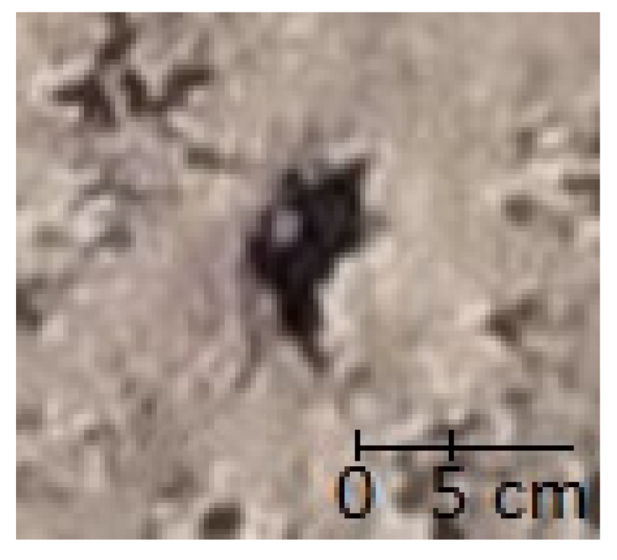
Description of vole burrows (Figure 3)—Entrances to the burrows (described here as holes and/or burrow holes) are normally 2.5–7.5 cm in diameter (Figure 4). Voles are social animals and create complex burrow systems with numerous entrances. Although the burrow entrances are typically oval, some collapse over time, especially once they are abandoned or empty after previous control measures, creating irregular shapes. Therefore, the proposed detection method should be tolerant to these shapes and slight changes.
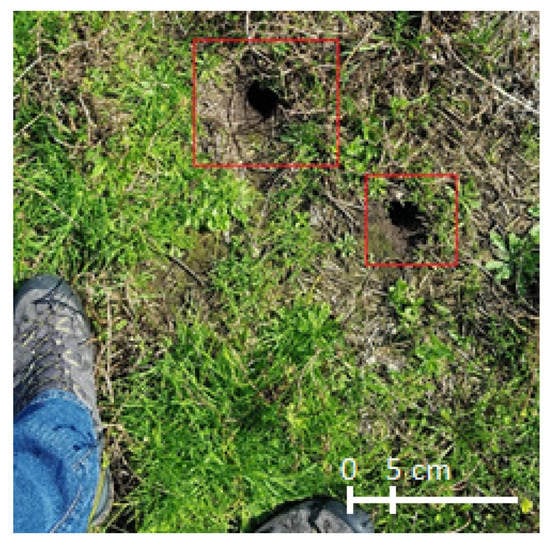
Figure 3.
Photo of oval-shaped burrow holes, marked in red rectangles, taken with a smartphone camera from a height of 1 m.
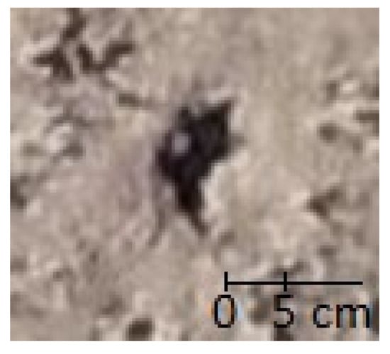
Figure 4.
Photo of a collapsed hole with an irregular shape, taken with a UI DJI Phantom 4 Pro camera, from a height of 30 m.
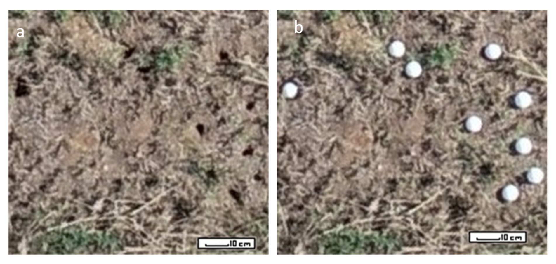
Validation—Data collection was divided into two stages: (i) photographing the plots for the first time; and (ii) photographing the plots for the second time, where all the vole burrows were counted and marked (in total 1740 burrows) with white Styrofoam balls, which were placed on the top of the burrows. This process was done to enable validation at a later stage, and only visible burrows were counted and marked (Figure 5), no covered burrows were taken into account. Moreover, to assure the exact location of the holes the DGPS was collected and marked only if appeared in a model (digital surface model DSM and orthophoto) created using Pix4D.
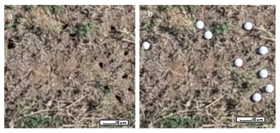
Figure 5.
External validation test data were collected via UAS before (a) and after (b) marking burrows with white Styrofoam balls.
The absolute vertical and horizontal accuracy of the UAS-based products (DSM and orthophoto) was comparable to that of the GPS device (several meters). This could be significantly improved using the DGPS system in the field (to cm level). With this in mind, a total of 10 ground control points (GCPs) were measured, which were well distributed throughout the field and near-visible horizontally and vertically important objects (pillars, weather station, etc.) [48].
Processing of UAS imagery—The images were processed using the structure from motion (SfM) method [49], implemented in Pix4D Mapper Pro (v. 4.3.31), which included all the main steps of this method. An automatic image quality module (implemented in MATLAB, using the horizontal and vertical components of the Sobel edge filter, and applied before the data were input to the SfM workflow) [50] was used to identify and remove all blurry images from the data folder [51] before the images were processed.
The common workflow for dense point cloud generation included posing estimation, image alignment, generation of tie points, generation of dense point clouds using dense stereo matching techniques such as the semi-global matching (SGM) algorithm [52], and 3D modeling [53]. The recommended parameters were used to generate dense point clouds (e.g., the ‘high’ option for dense point cloud generation) produced high-resolution orthophotos and DSMs with a spatial resolution of 1.5 cm. The point density option was set to ‘optimal’, and the minimum number of matches was set to three, using a matching window of size 9 × 9 pixels. Finally, the geometric accuracies of the generated point clouds and DSMs were evaluated separately. The visual features were illustrated using quantile-quantile plots [54], elevation profiles, and error classification maps [55]. The accuracy of the DSM was 2 cm in the horizontal direction, and <3 cm in the vertical direction, calculated based on five validation GPS points that were measured in the field (using an Emlid ReachRS2 device) but were not used in the Pix4D model. In this study, we used the “calibrated camera parameters file” and “calibrated external camera parameters” offered by the Pix4D [48].
Thematic layers—The DSM was processed further to create two additional inputs for the training of the CNN. The first product was a terrain ruggedness index (TRI) [50,56,57], which represents the mean of the absolute differences in height between a focal cell and its 3 × 3 neighboring cubes (ca. 4.5 cm3) and quantifies the total change. Smooth surfaces have a value of zero, while rough surfaces have positive values. This simple index was used as a normalization factor in further analysis, as it could categorize each surface using a simple scoring system (positive values).
Next, we calculated the texture, which is a descriptive property of all the surfaces and contains information regarding the structural arrangement of features and the relationship with their surroundings. Our main approach to the quantification of scene texture involved computation using a moving window with two-dimensional (2D) surface roughness as an input. Please note that in the processing stage, the point cloud was extracted using a 3D gray level co-occurrence matrix (GLCM). The 2D GLCM is a matrix, where each input datum has a gray level [58] examining the spatial relationship of objects. The 3D GLCM is used to determine the distance and direction before the pixel pairs are counted, whereas for the 2D GLCM, only horizontal distances and directions are determined before counting, and vertical distances are computed during the counting process. The specific generation process used in 3D GLCM [59] involves the following steps: (i) fix the image window size for a pixel and the level of intensity; (ii) define the horizontal distance and direction; (iii) split the vertical direction into sections, and prepare the same number of matrices; (iv) in the fixed window, find all pixel pairs that satisfy the condition in (ii); (v) compute the vertical direction for each pixel pair in (iii), meaning that each pixel pair will be counted in the corresponding matrix based on its vertical direction; (vi) generate the GLCM by counting in the same planar direction but in different vertical directions; (vii) compute Haralick features [60] to quantitatively describe the GLCM.
Evaluation metrics (Table 1)—The following four metrics were used to evaluate the classification model: precision, recall, F1-score, and mean average precision (mAP). These are defined based on four quantities: true positive (TP), which indicates that the predicted and actual values are both positive; false positive (FP), which means that the predicted value is positive, but the actual forecast is negative; false negative (FN), which means that the actual value is positive but the predicted value is negative; true negative (TN), which means that the predicted and actual values are both negative.

Table 1.
Evaluation metrics.
The intersection over union (IoU) measures the overlap ratio between the detected object (marked by a bounding box) and the ground truth (an annotated bounding box that is not included in the training dataset). The value of IoU varies between zero (no overlap) and one (total overlap) and is used to determine whether the detected object is a real object (according to a given threshold). The threshold in this study was very low (0.1), due to our interest in small objects.
The mean average precision (mAP) is defined as the integral of the precision over the recall interval [0, 1], i.e., the area under the precision-recall curve [61].
3.2.2. Training
The infrastructure used for training was a single NVIDIA® V10017 tensor core graphical processing unit (GPU) with 16 GB memory, as part of an NVIDIA® DGX-118 supercomputer for deep learning.
Faster R-CNN was pre-trained on MS-COCO [20] with a stochastic gradient descent optimizer with a momentum of 0.9 and a weight decay set to 0.0001. The learning rate was 0.01 in the first 500 iterations and then multiplied by 0.1 at epochs 10, 30, and 100.
The training of YOLO has been carried out in two stages: an initial training phase and a self-training phase. The initial stage used the original training data to train the model, while the self-training stage, also called pseudo-labeling, extended the available training data by inferring detections for images for which no original annotation data were available [62]. This was realized using the model resulting from the initial training stage, and the generated detections were then used as pseudo-annotated data.
Cross-validation was performed to approximate training optima using a default set of hyperparameters performed in the single-class training mode. In the initial training stage, a base model was trained on the training dataset for 100 epochs with a batch size of 30. This base model was initialized with weights from the pre-trained MS-COCO model.
In the self-training phase, the base model was used to create an extended training dataset. Pseudo-annotation data were inferred for the validation and test datasets using the best-performing epoch (which was automatically saved by the model). At this stage, the base model training was resumed from its latest epoch and was trained further on the extended training dataset with a batch size of 10.
The EfficientNet and RetinaNet models were trained on an NVIDIA Quadro RTX 8000 GPU with a batch size of 16, a stochastic gradient descent optimizer with a learning rate of 0.00005, a momentum of 0.9, and 50 epochs.
Each image obtained by the UAS was manually annotated by drawing rectangles to surround each object. A total of 6100 images of burrows were manually annotated for the training and test datasets, from which 4200 training samples and 1900 test samples were produced (~70% training, ~30% test). Furthermore, in total 1740 images were divided into two (~50–50%) groups (Figure 6) labeled background 1 (bare soil) and background 2 (ground cover) and used as an external validation (test sites).
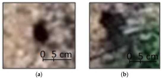
Figure 6.
Examples of holes with bare soil background (a) and ground cover (b).
4. Results
Table 2 and Table 3 show the results of the internal test for 30% of the input data (1900 test samples out of 6100 images in total) from various algorithms, focusing specifically on the detection rate for an orthophoto versus a single UAS image. Table 2 lists the training results for each method for a single UAS image. In terms of precision, recall, mAP, and F1-score, the performance of the self-trained YOLOv3 model was superior to the other six methods. Faster R-CNN, RetinaNet, YOLOv5 (self-trained and initially trained) and EfficientNet achieved lower results (mAP = 32%, 58%, 60%, 61% and 66%) than the general YOLOv3 model (mAP = 72%), and the self-trained YOLOv3 model (mAP = 82%). The results in Table 2 also confirm the good performance of YOLOv3 in terms of recall/precision balance. The best F1-score of 0.93 was achieved by the self-trained YOLOv3 model; this was significantly higher than the values for the other detectors, such as EfficientNet (0.80) and YOLOv5 self-training (0.76), RetinaNet (0.75), and Faster R-CNN (0.52).
Table 2.
Overall training evaluation metrics (best result in bold) for a single UAS image for 30% of the input data (1900 test samples out of 6100 images in total).
Table 3.
Overall training evaluation metrics (best result in bold) for an orthophoto product for 30% of the input data (1900 test samples out of 6100 images in total).
Table 3 presents the training results for each examined method for the orthophoto products. In terms of precision, recall, mAP, and F1 score, once again the performance of the self-trained YOLOv3 were superior to those of the other six methods, with a mAP of 0.81 and an F1-score of 84%, while the worst results were obtained by Faster R-CNN with a mAP of 0.33 and an F1-score of 52%.
Based on the results in Table 2 and Table 3, the following observations can be made: (i) the YOLOv3 models achieved better performance than the other models, thus demonstrating the advantage of the small target detector; (ii) the self-training model is beneficial to both YOLOv3 (the F1-score improved from 84% to 91% for a single UAS image product and 83% to 84% for an orthophoto product) and YOLOv5 (the F1-score improved from 76% to 78% for a single UAS image product and from 70% to 72% for an orthophoto product); and (iii) from a global perspective, the training results for all detectors were better for the single UAS image, as all detectors achieved lower performance for the orthophoto product.
Table 4 shows the effect of using DSM-related layers (with multimodal data as input). Following the approach suggested by Brook and Stober-Zisu (2020) for textural analysis, three thematic/textural maps calculated using 3D GLCM were tested based on homogeneity, entropy, and correlation. The multimodal dataset with three layers at once allowed us to train all the suggested models with the following input combinations: Dataset 1: grayscale orthophoto product, TRI (roughness), and a homogeneity layer (3D GLCM textural maps); Dataset 2: grayscale orthophoto product, TRI (roughness) layer and a correlation layer (3D GLCM textural maps); Dataset 3: grayscale orthophoto product, TRI (roughness) layer and an entropy layer (3D GLCM textural maps).
Table 4.
Overall training evaluation metrics (best result in bold) on multimodal datasets for an orthophoto product for 30% of the input data (1900 test samples out of 6100 images in total).
Compared with the original orthophoto training results (in Table 3), the multimodal input datasets achieved better results with Dataset 3. The results in Table 4 show that the self-training YOLOv3 fed with Dataset 3 achieved a mAP of 0.86 and an F1-score of ~94%, values that were significantly higher than those reported for a single UAS imagery product (Table 2).
Effects of Different Backgrounds in the Validation Sets
The detection of small objects with various agricultural backgrounds is a key challenge in many remote-sensing applications. To improve prediction accuracy, the training data should be captured in various environments so that the network can distinguish between the object of interest and background targets. An alternative approach is a model that can generalize the characteristics of the scene without prior knowledge regardless of their background/environment. The main aim here was to evaluate the ability of the initially trained and self-trained YOLOv3 model to handle a range of agricultural backgrounds. Two external validation areas (1740 samples in total) with new backgrounds (bare soil and groundcover backgrounds) were selected. Table 5 presents the results for all the products (i.e., a single UAS image, orthophoto, and multimodal dataset) on two different validation sets.
Table 5.
Overall external test evaluation metrics (best result in bold) on all available datasets for two validation sets (1740 samples in total).
As shown in Table 5, the self-trained YOLOv3 achieved better results for all input datasets (as shown in bold) on the first validation set (bare soil) than for the second (groundcover). This can be explained by the level of similarity between the backgrounds in the validation set and the training set. The groundcover (training set) was more similar to the bare soil (validation set 1) than to the groundcover (validation set 2). When comparing the results with those reported in Table 4, where the self-trained YOLOv3 achieved a mAP of 0.86 for the multimodal dataset, the performance for unseen backgrounds in the validation set was lower (i.e., in 3% for the bare soil and 8% for the groundcover background). Compared to the other input datasets, this model achieved the best performance (i.e., 6% on the first background and 12% on the second background for the orthophoto product and 8% on the first background, and 9% on the second background for a single UAS image).
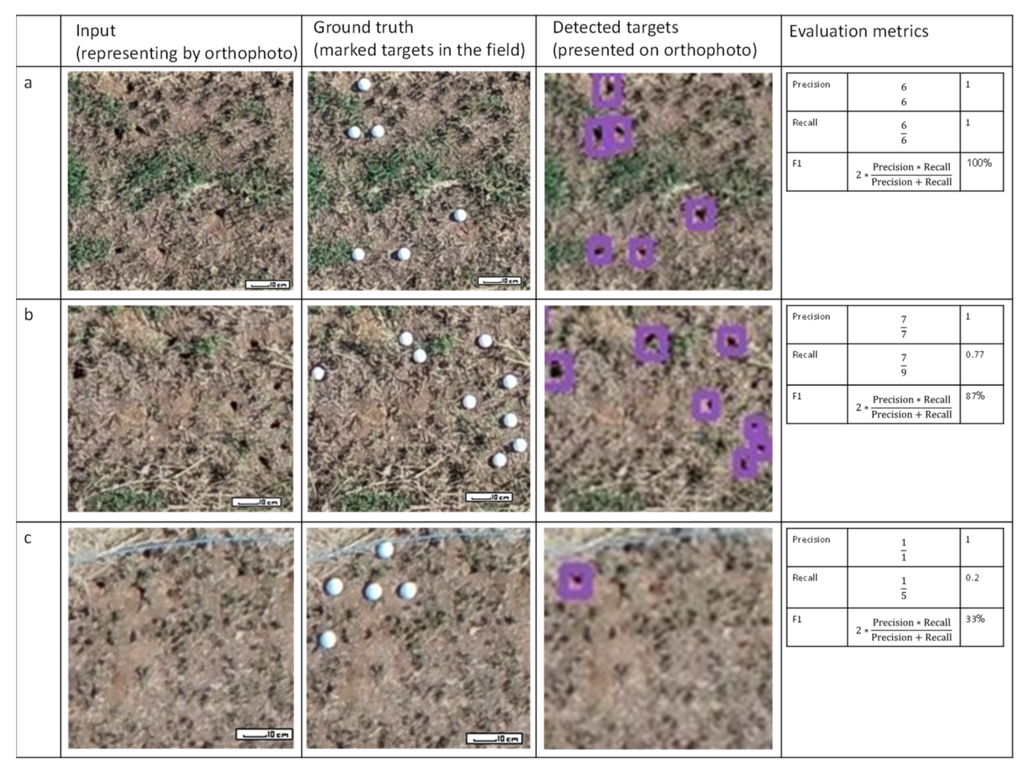
In (Figure 7) three examples of detection level for the external test sites are presented in subsets. In Figure 7a the reported results achieved the best level of detection with F1-score of 100%, in b the detection level is lower ~87% and in c the detection level is very low 33%. These results representing the best, moderate, and worst results of the model.

Figure 7.
Selected examples of detection level for the external test sites, (a) the best; (b) the moderate; and (c) the worst, results of the model.
The multimodal dataset (i.e., grayscale orthophoto product, TRI roughness index layer, and the entropy layer calculated via 3D GLCM textural information) produced the most accurate results. However, comparing between orthophoto product and single UAS image data, the results in Table 2 and Table 3 show that a single UAS image product is advantageous, as it was able to detect vole burrows better than an orthophoto product. This may be due to the spatial resolution and to the spatial/geometrical artifacts and general smoothness, particularly at the edges, produced by the triangulation/interpolation processes in the photogrammetric program. However, the multimodal dataset that included the orthophoto product and was supported using two physical surface properties (i.e., the roughness and texture randomness, calculated as surface entropy) derived from the DSM model yielded the best results. These findings illustrate the effectiveness and influence of multimodal datasets on machine learning and the rate of detection of small objects from low-cost UAS-based sensors.
5. Discussion
The detection of small objects with various agricultural backgrounds is a key challenge in many remote-sensing applications. Several methods and deep learning algorithms can be addressed to detect objects, but not all of them can accurately detect small objects, especially objects with various agricultural backgrounds [63] in UAS-based remote-sensing imagery.
On an operational level, the best time to collect the field data and capture detailed information is immediately after the harvest, before the groundcover or small weeds start growing around the burrows and change the background. This is a preferable time window to assure significantly easier and more accurate target detection. Indeed, an important influencing factor in the practical applications of remote-sensing means for small object detection is reclined on testing different types of input datasets.
In this study were tested three different input datasets were: (i) single UAS images, (ii) orthophotos, (iii) multimodal dataset (combining textural physical layers with orthophoto data), on one- and two-stage algorithms such as YOLOv3 and Faster-RCNN respectively.
The YOLO v3 algorithm achieved better results than other examined methods. Evaluated by metrics of precision, recall, mAP, and F1-score, the performance of the self-trained YOLOv3 model was superior to the other six methods (Table 2, Table 3 and Table 4). This model demonstrated an excellent ability of a one-stage algorithm to detect small (vary in shape) targets in a complex agricultural background. The self-training model was beneficial to both YOLOv3 (the F1-score improved from 84% to 91% for a single UAS image product and 83% to 84% for an orthophoto product) and YOLOv5 (the F1-score improved from 76% to 78% for a single UAS image product and from 70% to 72% for an orthophoto product). The training results for all detectors were better for the single UAS image, as all detectors achieved lower performance for the orthophoto product (Table 2 and Table 3). On the other hand, research that tested the capability of YOLOv3 and YOLOv5 for apple picking robot [64], concluded that the average time for one apple detection is about 19 ms for YOLOv3. Both speed and error fractions were less than in all known similar applications. YOLOv5 in this type of application, detected apples precisely without any additional techniques [64]. Numerous studies searched for a reason causing small object miss-detection and false detection [65]. Several studies compare YOLOv5 and YOLOv3, but only after improving the initial anchor box size of the original YOLOv5network to avoid misrecognition of small objects [66]. However, in our study, the targets are small and probably not in contrast to YOLOv5, therefore this model could not outperform the 3rd version of YOLO.
In addition, the average detection speeds per orthophoto (field area of 24 × 40 m with 1.5 spatial resolution) is ~50 times longer than the detection process time for a single UAS image [67]. This fact is important for practical applications and should be taken into account in the case of emergency or under a normal agriculture schedule that every action should be on time. The main benefit of a single UAS image detector based on YOLOv3 is its computational time. The external test dataset reported the following detection speed: (i) a single UAS image was processed around 0.05 s, which was very fast compared to orthophoto or multimodal inputs (execution time); (ii) a single orthophoto was processed around 3 min; and (iii) multimodal was processed around 3.5 min, this calculation is not considering the data preparation time, i.e., Pix4D Mapper, 3D GLCM, etc.
The multimodal input datasets achieved the best results with the grayscale orthophoto product, TRI (roughness) layer, and an entropy layer (3D GLCM textural maps) dataset (Table 4) for the self-training YOLOv3 model (mAP of 0.86 and an F1-score of ~94%). Its results were significantly higher than those reported for both multimodal grayscale datasets and higher than a single UAS imagery dataset. Image texture and physical layers provided valuable information on the spatial arrangement, and together with shade (in our case grayscale) or intensities were selected as the most informative and suitable input dataset, similarly to studies [68] reporting on the advantages of multimodal for small object detection.
To improve prediction accuracy and more importantly to support a real-world application, the model should be able to operate under various environments so that the network can distinguish between the object of interest and background [69]. Our original hypothesis that “the target objects on the bare soil backgrounds will be easier to detect” has been tested. Indeed, according to Table 5, the self-trained YOLOv3 achieved better results for all input datasets on the first validation set (bare soil) than for the second (groundcover). This can be explained by the level of similarity between the backgrounds in the validation set and the training set. The groundcover (training set) was more similar to the bare soil (external test—validation set 1) than to the groundcover (external test—validation set 2). When comparing the results with those reported in Table 4, where the self-trained YOLOv3 achieved a mAP of 0.86 for the multimodal dataset, the performance for unseen backgrounds in the validation set was lower (i.e., in 3% for the bare soil and 8% for the groundcover background). Compared to the other input datasets, this model achieved the best performance (i.e., 6% on the bare soil background and 12% on the groundcover background for the orthophoto product and 8% on the first background, and 9% on the second background for a single UAS image).
6. Conclusions
One and two-stage detector models usable to detect small targets in agricultural backgrounds, from different input datasets, have been examined to identify an environmentally efficient method of rodent control to support the achievement of SDG2 and to promote sustainable agriculture. The focus of this study was on evaluating the performance of the suggested models on a single UAS-based image, a UAS-based orthophoto product processed with the Pix4D mapper photogrammetric program, and a multimodal product for agriculture/environmental applications. The contribution of the multimodal dataset to small object detection was assessed and reported. A study and analysis of a field-scale (real-world) UAS dataset using Faster R-CNN, YOLOv3, YOLOv5, EfficientNet, and RetinaNet showed that the highest mAP value and F1-score were achieved by the self-trained YOLOv3 on multimodal data. The validation results demonstrated the superiority and practicality of the multimodal dataset. The main conclusions of this work are as follows:
Superior results were obtained from high spatial resolution edge/contrast-preserving data (single UAS-based imagery) than from an orthophoto produced by a photogrammetry program. These data showed a relatively high detection rate of vole burrows (small targets), but this method is not efficient at the field scale. Although its performance was poorer, the orthophoto also showed potential as a detection method. The use of physical/texture information showed great promise in terms of the detection of vole burrows from a multimodal dataset, and achieved higher prediction accuracy when all the spatial and physical features were included.
Multimodal data yielded superior performance in the detection of vole burrows compared to single UAS image data, for all modeling methods.
A self-trained multimodal YOLOv3 model outperformed the other methods and exhibited strong adaptability to different datasets with high detection accuracy, along with robustness in terms of spatial dependency and variation.
Author Contributions
Data collection, H.E., M.C.; Analysis, H.E., A.B. (Anna Brook); Interpretation, H.E., A.B. (Anna Brook); Writing the manuscript, H.E., A.B. (Anna Brook); Data preparation, A.B. (Anna Brook); Connecting the topic to SDG and EU level, A.B. (Antonello Bonfante), A.B. (Anna Brook); General supervision, M.C., A.B. (Anna Brook). All authors have read and agreed to the published version of the manuscript.
Funding
This research was funded by the Ministry of Agriculture and Rural Development, State of Israel, grant number 60-02-0003.
Institutional Review Board Statement
Not applicable.
Informed Consent Statement
Not applicable.
Data Availability Statement
Not applicable.
Acknowledgments
The project was funded by the Ministry of Agriculture and Rural Development, State of Israel (Grant number 60-02-0003). The authors would like to acknowledge Cost Action CA16219 (Harmonization of UAS techniques for agricultural and natural ecosystems monitoring) for professional and technical guidance. We are grateful to the Shamir research institute for technical support during field campaigns and data collection.
Conflicts of Interest
The authors declare no conflict of interest.
References
- FAO. Conference STRATEGIC FRAMEWORK 2010–2019, C 2009/3. 2009. [Online]. Available online: www.fao.orgW/K5864/e (accessed on 23 November 2009).
- Stenseth, N.C.; Leirs, H.; Skonhoft, A.; Davis, S.A.; Pech, R.P.; Andreassen, H.P.; Singleton, G.R.; Lima, M.; Machang’u, R.S.; Makundi, R.H.; et al. Mice, rats, and people: The bio-economics of agricultural rodent pests. Front. Ecol. Environ. 2003, 1, 367–375. [Google Scholar] [CrossRef]
- Buckle, A.; Smith, R. Rodents in agriculture and forestry. In Rodent Pests Control; Buckle, A.P., Smith, R.H., Eds.; School of Biological Sciences, University of Reading: Reading, UK, 2015; pp. 33–80. [Google Scholar]
- Liang, X.; Zhang, J.; Zhuo, L.; Li, Y.; Tian, Q. Small Object Detection in Unmanned Aerial Vehicle Images Using Feature Fusion and Scaling-Based Single Shot Detector with Spatial Context Analysis. IEEE Trans. Circuits Syst. Video Technol. 2019, 30, 1758–1770. [Google Scholar] [CrossRef]
- Jones, P.V.M.J. Robust Real-time Object Detection. Int. J. Comput. Vis. 2001, 4, 34–47. [Google Scholar]
- Gu, Y.; Wylie, B.K.; Boyte, S.P.; Picotte, J.; Howard, D.M.; Smith, K.; Nelson, K.J. An Optimal Sample Data Usage Strategy to Minimize Overfitting and Underfitting Effects in Regression Tree Models Based on Remotely-Sensed Data. Remote Sens. 2016, 8, 943. [Google Scholar] [CrossRef] [Green Version]
- Al-Najjar, H.A.H.; Kalantar, B.; Pradhan, B.; Saeidi, V.; Halin, A.A.; Ueda, N.; Mansor, S. Land Cover Classification from fused DSM and UAV Images Using Convolutional Neural Networks. Remote Sens. 2019, 11, 1461. [Google Scholar] [CrossRef] [Green Version]
- Zhang, X.; Han, L.; Han, L.; Zhu, L. How Well Do Deep Learning-Based Methods for Land Cover Classification and Object Detection Perform on High Resolution Remote Sensing Imagery? Remote Sens. 2020, 12, 417. [Google Scholar] [CrossRef] [Green Version]
- Jogin, M.; Mohana; Madhulika, M.S.; Divya, G.D.; Meghana, R.K.; Apoorva, S. Feature Extraction using Convolution Neural Networks (CNN) and Deep Learning. In Proceedings of the 3rd IEEE International Conference on Recent Trends in Electronics, Information & Communication Technology (RTEICT), Bengaluru, India, 18–19 May 2018; pp. 2319–2323. [Google Scholar]
- Girshick, R.; Donahue, J.; Darrell, T.; Malik, J. Region-Based Convolutional Networks for Accurate Object Detection and Segmentation. IEEE Trans. Pattern Anal. Mach. Intell. 2015, 38, 142–158. [Google Scholar] [CrossRef] [PubMed]
- Girshick, R. Fast R-CNN. In Proceedings of the IEEE International Conference on Computer Vision, Santiago, Chile, 7–13 December 2015; pp. 1440–1448. [Google Scholar] [CrossRef]
- Dai, J.; Li, Y.; He, K.; Sun, J. R-FCN: Object detection via region-based fully convolutional networks. arXiv 2016, arXiv:1605.06409. [Google Scholar]
- Dyrmann, M.; Jørgensen, R.N.; Midtiby, H.S. RoboWeedSupport-Detection of weed locations in leaf occluded cereal crops using a fully convolutional neural network. Adv. Anim. Biosci. 2017, 8, 842–847. [Google Scholar] [CrossRef]
- Dias, D.; Dias, U. Flood detection from social multimedia and satellite images using ensemble and transfer learning with CNN architectures. In Proceedings of the CEUR Workshop Proceedings, Sophia Antipolis, France, 29–31 October 2018; p. 2283. [Google Scholar]
- Bargoti, S.; Underwood, J. Image classification with orchard metadata. In Proceedings of the 2016 IEEE International Conference on Robotics and Automation (ICRA), Stockholm, Sweden, 16–21 May 2016; Institute of Electrical and Electronics Engineers (IEEE), Australian Centre for Field Robotics: Sydney, Australia, 2016; pp. 5164–5170. [Google Scholar]
- Kamilaris, A.; Prenafeta-Boldú, F.X. Deep learning in agriculture: A survey. Comput. Electron. Agric. 2018, 147, 70–90. [Google Scholar] [CrossRef] [Green Version]
- Law, H.; Deng, J. CornerNet: Detecting objects as paired keypoints. In Proceedings of the European Conference on Computer Vision (ECCV), Munich, Germany, 8–14 September 2018; pp. 734–750. [Google Scholar]
- Shen, Z.; Liu, Z.; Li, J.; Jiang, Y.-G.; Chen, Y.; Xue, X. DSOD: Learning Deeply Supervised Object Detectors from Scratch. In Proceedings of the 2017 IEEE International Conference on Computer Vision, Venice, Italy, 22–29 October 2017; pp. 1937–1945. [Google Scholar]
- Lin, T.Y.; Goyal, P.; Girshick, R.; He, K.; Dollár, P. Focal Loss for Dense Object Detection. In Proceedings of the IEEE International Conference on Computer Vision, Venice, Italy, 22–29 October 2017; pp. 2999–3007. [Google Scholar]
- Lin, T.-Y.; Maire, M.; Belongie, S.; Hays, J.; Perona, P.; Ramanan, D.; Dollár, P.; Zitnick, C.L. Microsoft COCO: Common Objects in Context. In Computer Vision–ECCV 2014.; Springer: Cham, Switzerland, 2014; pp. 740–755. [Google Scholar] [CrossRef] [Green Version]
- Redmon, J.; Divvala, S.; Girshick, R.; Farhadi, A. You Only Look Once: Unified, Real-Time Object Detection. In Proceedings of the IEEE Conference on Computer Vision and Pattern Recognition, Las Vegas, NV, USA, 27–30 June 2016; pp. 779–788. [Google Scholar] [CrossRef] [Green Version]
- Redmon, J.; Farhadi, A. YOLO v3.0: An Incremental Improvement. arXiv 2018, arXiv:1804.02767. [Google Scholar]
- Hua, Y.; Mou, L.; Zhu, X.X. LAHNet: A Convolutional Neural Network Fusing Low- and High-Level Features for Aerial Scene Classification. In Proceedings of the IGARSS 2018-2018 IEEE International Geoscience and Remote Sensing Symposium, Valencia, Spain, 22–27 July 2018; pp. 4728–4731. [Google Scholar]
- Lu, X.; Li, Q.; Li, B.; Yan, J. MimicDet: Bridging the Gap Between One-Stage and Two-Stage Object Detection. arXiv 2020, arXiv:2009.11528. [Google Scholar]
- Pham, V.; Pham, C.; Dang, T. Road Damage Detection and Classification with Detectron2 and Faster R-CNN. In Proceedings of the 2020 IEEE International Conference on Big Data (Big Data) 2020, Atlanta, GA, USA, 10–13 December 2020; pp. 5592–5601. [Google Scholar]
- Benton, T.; Vickery, J.A.; Wilson, J. Farmland biodiversity: Is habitat heterogeneity the key? Trends Ecol. Evol. 2003, 18, 182–188. [Google Scholar] [CrossRef]
- Witmer, G.W.; Moulton, R.S.; Baldwin, R.A. An efficacy test of cholecalciferol plus diphacinone rodenticide baits for California voles (Microtus californicusPeale) to replace ineffective chlorophacinone baits. Int. J. Pest Manag. 2014, 60, 275–278. [Google Scholar] [CrossRef]
- Kross, S.M.; Bourbour, R.; Martinico, B. Agricultural land use, barn owl diet, and vertebrate pest control implications. Agric. Ecosyst. Environ. 2016, 223, 167–174. [Google Scholar] [CrossRef]
- Motro, Y. Economic evaluation of biological rodent control using barn owls Tyto alba in alfalfa. In Proceedings of the Julius-Kühn-Archiv 8 th European Vertebrate Pest Management Conference, Berlin, Germany, 26–30 September 2011; pp. 79–80. [Google Scholar] [CrossRef]
- Cohen-Shlagman, L.; Hellwing, S.; Yom-Tov, Y. The biology of the Levant vole, Microtus guentheri in Israel. II. The reproduction and growth in captivity. Z. Für Säugetierkd. 1984, 49, 148–156. [Google Scholar]
- Cohen-Shlagman, L.; Hellwing, S.; Yom-Tov, Y. The biology of the Levant vole, Microtus guentheri in Israel. I: Population dynamics in the field. Z. Für Säugetierkd. 1984, 49, 135–147. [Google Scholar]
- Yom-Tov, Y.; Yom-Tov, S.; Moller, H. Competition, coexistence, and adaptation amongst rodent invaders to Pacific and New Zealand islands. J. Biogeogr. 1999, 26, 947–958. [Google Scholar] [CrossRef] [Green Version]
- US EPA; Grube, A.; Donaldson, D.; Kiely, T.; Wu, L. Pesticides Industry Sales and Usage; US EPA: Washington, DC, USA, 2011; p. 41. [Google Scholar]
- Stone, W.B.; Okoniewski, J.C.; Stedelin, J.R. Poisoning of Wildlife with Anticoagulant Rodenticides in New York. J. Wildl. Dis. 1999, 35, 187–193. [Google Scholar] [CrossRef] [PubMed]
- Terrell, P.S.; Salmon, T.P.; Lawrence, S.J. Anticoagulant Resistance in Meadow Voles (Microtus californicus). Proc. Proc. Vertebr. Pest Conf. 2006, 22. [Google Scholar] [CrossRef] [Green Version]
- Buckle, A. Anticoagulant resistance in the United Kingdom and a new guideline for the management of resistant infestations of Norway rats (Rattus norvegicusBerk.). Pest Manag. Sci. 2013, 69, 334–341. [Google Scholar] [CrossRef]
- Meyrom, K.; Motro, Y.; Leshem, Y.; Aviel, S.; Izhaki, I.; Argyle, F.; Charter, M. Nest-box use by the Barn Owl Tyto alba in a biological pest control program in the Beit She’an valley, Israel. Ardea 2009, 97, 463–467. [Google Scholar] [CrossRef]
- Peleg, O.; Nir, S.; Leshem, Y.; Meyrom, K.; Aviel, S.; Charter, M.; Roulin, A.; Izhak, I. Three Decades of Satisfied Israeli Farmers: Barn Owls (Tyto alba) as Biological Pest Control of Rodents. Proc. Proc. Vertebr. Pest Conf. 2018, 28. [Google Scholar] [CrossRef] [Green Version]
- Khosla, R. Precision agriculture: Challenges and opportunities in a flat world. In Proceedings of the Soil Solutions for a Changing World, Brisbane, Australia, 1–6 August 2020. [Google Scholar]
- Zhang, C.; Kovacs, J.M. The application of small unmanned aerial systems for precision agriculture: A review. Precis. Agric. 2012, 13, 693–712. [Google Scholar] [CrossRef]
- Ren, S.; He, K.; Girshick, R.; Sun, J. Faster R-CNN: Towards Real-Time Object Detection with Region Proposal Networks. IEEE Trans. Pattern Anal. Mach. Intell. 2015, 39, 1137–1149. [Google Scholar] [CrossRef] [PubMed] [Green Version]
- Chen, Z.; Xie, Z.; Zhang, W.; Xu, X. ResNet and Model Fusion for Automatic Spoofing Detection. Interspeech 2017, 102–106. [Google Scholar] [CrossRef] [Green Version]
- Lin, T.-Y.; Dollar, P.; Girshick, R.; He, K.; Hariharan, B.; Belongie, S. Feature Pyramid Networks for Object Detection. In Proceedings of the 2017, IEEE Conference on Computer Vision and Pattern Recognition (CVPR), Honolulu, HI, USA, 21–26 July 2017; pp. 936–944. [Google Scholar] [CrossRef] [Green Version]
- Pham, M.-T.; Courtrai, L.; Friguet, C.; Lefèvre, S.; Baussard, A. YOLO-Fine: One-Stage Detector of Small Objects under Various Backgrounds in Remote Sensing Images. Remote Sens. 2020, 12, 2501. [Google Scholar] [CrossRef]
- Wang, C.Y.; Bochkovskiy, A.; Liao, H.Y.M. Scaled-YOLOv4: Scaling Cross Stage Partial Network. arXiv 2020, arXiv:2011.08036. [Google Scholar]
- Liu, S.; Qi, L.; Qin, H.; Shi, J.; Jia, J. Path Aggregation Network for Instance Segmentation. In Proceedings of the 2018, IEEE/CVF Conference on Computer Vision a8759&nd Pattern Recognition (CVPR), Salt Lake City, UT, USA, 18–23 June 2018; Institute of Electrical and Electronics Engineers (IEEE): New York, NY, USA, 2018; pp. 8759–8768. [Google Scholar] [CrossRef] [Green Version]
- He, K.; Zhang, X.; Ren, S.; Sun, J. Spatial pyramid pooling in deep convolutional networks for visual recognition. IEEE Trans. Pattern Anal. Mach. Intell. 2015, 37, 1904–1916. [Google Scholar] [CrossRef] [Green Version]
- Tmušić, G.; Manfreda, S.; Aasen, H.; James, M.R.; Gonçalves, G.; Ben-Dor, E.; Brook, A.; Polinova, M.; Arranz, J.J.; Mészáros, J.; et al. Current Practices in UAS-based Environmental Monitoring. Remote Sens. 2020, 12, 1001. [Google Scholar] [CrossRef] [Green Version]
- Boon, M.A.; Greenfield, R.; Tesfamichael, S. Wetland assessment using unmanned aerial vehicle (uav) photogrammetry. ISPRS -Int. Arch. Photogramm. Remote. Sens. Spat. Inf. Sci. 2016, XLI-B1, 781–788. [Google Scholar] [CrossRef] [Green Version]
- Brook, A.; Shtober-Zisu, N. Rock surface modeling as a tool to assess the morphology of inland notches, Mount Carmel, Israel. Catena 2020, 187, 104256. [Google Scholar] [CrossRef]
- Sieberth, T.; Wackrow, R.; Chandler, J.H. Automatic detection of blurred images in UAV image sets. ISPRS J. Photogramm. Remote Sens. 2016, 122, 1–16. [Google Scholar] [CrossRef] [Green Version]
- Hirschmüller, H. Semi-Global Matching Motivation, Developments and Applications. In Proceedings of the Photogramm Week, Stuttgart, Germany, 5–9 September 2011. [Google Scholar]
- Alidoost, F.; Arefi, H. An Image-Based Technique For 3d Building Reconstruction Using Multi-View Uav Images. ISPRS-Int. Arch. Photogramm. Remote Sens. Spat. Inf. Sci. 2015, XL-1/W5, 43–46. [Google Scholar] [CrossRef] [Green Version]
- Höhle, J.; Höhle, M. Accuracy assessment of digital elevation models by means of robust statistical methods. ISPRS J. Photogramm. Remote Sens. 2009, 64, 398–406. [Google Scholar] [CrossRef] [Green Version]
- Ivelja, T.; Bechor, B.; Hasan, O.; Miko, S.; Sivan, D.; Brook, A. Improving vertical accuracy of uav digital surface models by introducing terrestrial laser scans on a point-cloud level. ISPRS Int. Arch. Photogramm. Remote Sens. Spat. Inf. Sci. 2020, XLIII-B1-2, 457–463. [Google Scholar] [CrossRef]
- Glenn, N.; Streutker, D.R.; Chadwick, D.J.; Thackray, G.D.; Dorsch, S.J. Analysis of LiDAR-derived topographic information for characterizing and differentiating landslide morphology and activity. Geomorphology 2006, 73, 131–148. [Google Scholar] [CrossRef]
- Berti, M.; Corsini, A.; Daehne, A. Comparative analysis of surface roughness algorithms for the identification of active landslides. Geomorphology 2013, 182, 1–18. [Google Scholar] [CrossRef]
- Soh, L.-K.; Tsatsoulis, C. Texture analysis of SAR sea ice imagery using gray level co-occurrence matrices. IEEE Trans. Geosci. Remote Sens. 1999, 37, 780–795. [Google Scholar] [CrossRef] [Green Version]
- Yan, L.; Xia, W. A modified three-dimensional gray-level co-occurrence matrix for image classification with digital surface model. ISPRS-Int. Arch. Photogramm. Remote Sens. Spat. Inf. Sci. 2019, XLII-2/W13, 133–138. [Google Scholar] [CrossRef] [Green Version]
- Kurani, A.S.; Xu, D.H.; Furst, J.; Raicu, D.S. Co-occurrence matrices for volumetric data. In Proceedings of the Seventh IASTED International Conference on Computer Graphics and Imaging, Kauai, HI, USA, 17–19 August 2004; pp. 426–443. [Google Scholar]
- Flach, P.A.; Kull, M. Precision-Recall-Gain curves: PR analysis done right. In Proceedings of the Advances in Neural Information Processing Systems 28 (NIPS 2015), Montreal, QC, Canada, 7–12 December 2015. [Google Scholar]
- Koitka, S.; Friedrich, C.M. Optimized Convolutional Neural Network Ensembles for Medical Subfigure Classification. Comput. Vis. 2017, 57–68. [Google Scholar] [CrossRef]
- Razakarivony, S.; Jurie, F. Vehicle detection in aerial imagery: A small target detection benchmark. J. Vis. Commun. Image Represent. 2016, 34, 187–203. [Google Scholar] [CrossRef] [Green Version]
- Kuznetsova, A.; Maleva, T.; Soloviev, V. Detecting Apples in Orchards Using YOLOv3 and YOLOv5 in General and Close-Up Images. In Proceedings of the Advances in Neural Networks—ISNN 2020, Cairo, Egypt, 4–6 December 2020; pp. 233–243. [Google Scholar] [CrossRef]
- Liu, M.; Wang, X.; Zhou, A.; Fu, X.; Ma, Y.; Piao, C. UAV-YOLO: Small Object Detection on Unmanned Aerial Vehicle Perspective. Sensors 2020, 20, 2238. [Google Scholar] [CrossRef] [Green Version]
- Yan, B.; Fan, P.; Lei, X.; Liu, Z.; Yang, F. A Real-Time Apple Targets Detection Method for Picking Robot Based on Improved YOLOv. Remote Sens. 2021, 13, 1619. [Google Scholar] [CrossRef]
- Jeon, I.; Ham, S.; Cheon, J.; Klimkowska, A.M.; Kim, H.; Choi, K.; Lee, I. A REAL-TIME DRONE MAPPING PLATFORM FOR MARINE SURVEILLANCE. ISPRS Int. Arch. Photogramm. Remote. Sens. Spat. Inf. Sci. 2019, 42, 385–391. [Google Scholar] [CrossRef] [Green Version]
- Shapiro, L.G.; Stockman, G.C. Motion from 2D Image Sequences. Comput. Vis. 2001, 9, 1–3. [Google Scholar]
- Bindu, S.; Prudhvi, S.; Hemalatha, G.; Sekhar, N.R.; Nanchariah, M.V. Object Detection from Complex Background Image Using Circular Hough Transform. J. Eng. Res. Appl. 2014, 4, 23–28. Available online: www.ijera.com (accessed on 15 April 2014).


Publisher’s Note: MDPI stays neutral with regard to jurisdictional claims in published maps and institutional affiliations. |
© 2021 by the authors. Licensee MDPI, Basel, Switzerland. This article is an open access article distributed under the terms and conditions of the Creative Commons Attribution (CC BY) license (https://creativecommons.org/licenses/by/4.0/).