Abstract
During the imaging process, hyperspectral image (HSI) is inevitably affected by various noises, such as Gaussian noise, impulse noise, stripes or deadlines. As one of the pre-processing steps, the removal of mixed noise for HSI has a vital impact on subsequent applications, and it is also one of the most challenging tasks. In this paper, a novel spectral-smoothness and non-local self-similarity regularized subspace low-rank learning (termed SNSSLrL) method was proposed for the mixed noise removal of HSI. First, under the subspace decomposition framework, the original HSI is decomposed into the linear representation of two low-dimensional matrices, namely the subspace basis matrix and the coefficient matrix. To further exploit the essential characteristics of HSI, on the one hand, the basis matrix is modeled as spectral smoothing, which constrains each column vector of the basis matrix to be a locally continuous spectrum, so that the subspace formed by its column vectors has continuous properties. On the other hand, the coefficient matrix is divided into several non-local block matrices according to the pixel coordinates of the original HSI data, and block-matching and 4D filtering (BM4D) is employed to reconstruct these self-similar non-local block matrices. Finally, the formulated model with all convex items is solved efficiently by the alternating direction method of multipliers (ADMM). Extensive experiments on two simulated datasets and one real dataset verify that the proposed SNSSLrL method has greater advantages than the latest state-of-the-art methods.
1. Introduction
Hyperspectral image (HSI) has played an important role in many modern scenarios like urban planning, agricultural exploration, criminal investigation, military surveillance, etc. [1]. However, the existing mixed noise generated during the process of digital imaging, e.g., Gaussian noise, salt and pepper, stripes and deadlines, seriously diminishes the accuracy of the above applications [2]. In addition, a series of HSI processing applications (e.g., unmixing [3,4], classification [5,6,7], super-resolution [8], target detection [9,10]) are greatly dependent on the imaging quality of HSI. Therefore, as a key preprocessing step of the above-mentioned applications, the studies on HSI mixed denoising methods have become a hot research topic and aroused widespread interest in the field.
Now, many methods of HSI denoising have been proposed. As each band of HSI can be regarded as a two-dimensional matrix, the simplest way is to directly use the traditional and classic two-dimensional image denoising method, such as Total Variation (TV) [11], K-SVD [12], NLM [13], BM3D [14], WNNM [15]. Part of the methods are based on the domain transform theory, that is, data are transformed from the original spatial domain to a transform domain for denoising, and then the denoising results are inversely transformed to the spatial domain, for example, based on curvelet transform [16], wavelet transform [17], principal component analysis (PCA) [18]. However, the disadvantage of these methods is that they ignore the strong correlation between the spatial dimension and spectral dimension of HSI, which leads to a poor denoising effect [19]. Therefore, to make full use of spectral and spatial information, a series of methods are proposed. On the basis of BM3D [14], Maggioni et al. [20] proposed BM4D method by using nonlocal similarity and Wiener filtering. Compared with using TV [21] method in each band, the adaptive TV method is applied to the spatial-spectral dimension in [22,23], which improves the denoising effect. Similarly, Qian et al. [24] proposed a local spatial structure sparse representation method to denoise HSI in groups. However, although the above-mentioned traditional denoising methods have good performance on HSI denoising, they work insufficiently well when the noise intensity is large and the noise category is specific, such as deadlines and stripes.
Recently, deep learning techniques and convolutional neural networks (CNN) have made great achievements in visual tasks, e.g., image classification [25,26,27,28], object detection [29,30,31], image forensics [32,33,34,35] and semantic segmentation [36,37,38]. Moreover, CNN is also used for various image restoration tasks [39,40,41,42], especially for denoising HSI [43,44]. In these methods, strict encoding and decoding structures [43] are adopted to construct a deep convolutional neural network through end-to-end training mode. Due to the ability of CNN to learn the nonlinear mapping function from a large amount of training data [45], the methods based on CNN also obtain fine denoising results. CNN has been extended for HSI denoising in [44]. However, each spectral band was denoised separately, and the spectral correlation between HSI is not fully utilized. These approaches model HSI by learning the multichannel features with two-dimensional convolution, which loses the rich information of spectral dimension. Different from the previous deep learning method that always takes two-dimensional convolution as the basic operation of the network, Wei et al. [46] introduces a three-dimensional convolution and a quasi-recurrent pooling function, which makes full use of the rich spectral information in HSI, thus significantly improving the accuracy and efficiency of the model.
In recent years, low-rank matrix restoration (LRMR) has become an important method of HSI restoration. This method involves learning low dimensional subspace from high dimensional data [47]. The most representative is the HSI denoising method based on LRMR proposed by Zhang et al. [48]. Xu [49] introduces a low-rank regularizer, which uses matrix factorization and weighted nuclear norm to better approximate the original low-rank hypothesis. However, in this framework, singular value decomposition is needed to solve these weighted kernel norm optimization problems. Not only is the computational complexity of the algorithm relatively high, but it is also not robust to the removal of mixed noises [50]. To solve these problems, Cao et al. [51] adaptively fit the noise through the exponential power distribution of the mixed noise, and proposed a more flexible method to apply in HSI mixed denoising. However, HSI is three-dimensional data and the spectral relationship between different bands is ignored based on matrix decomposition. The algorithm based on low-rank tensor decomposition maintains the global structure of hyperspectral data. A series of HSI restoration methods based on tensor decomposition have been proposed. For example, using CANDECOMP/PARAFAC (CP) decomposition [52], Tucker decomposition [53] and tensor-SVD decomposition [54] to establish the HSI restoration model, the noise removal results have been greatly improved. On this basis, people use various regularization methods to explore its prior. For example, Wang et al. [55] introduced Total Variation (TV) regularization into the low-rank tensor restoration framework to preserve the spatial piecewise smoothness. Sun et al. [56] propose a non-local enabled tensor subspace low-rank learning strategy to achieve mixed denoising. Lin et al. [57] introduce a deep prior to the low-rank decomposition framework to explore the nonlinear property of noise. Zheng et al. [58] propose a tensor fiber rank model for HSI mixed noise removal to explore the high-order low-rankness of HSI.
Although the above-mentioned methods have achieved a certain effect on the problem of mixed denoising, directly processing the original HSI often leads to inefficient execution of the algorithm, which is extremely fatal in real applications. In this paper, a spectral-smoothness regularized subspace low-rank learning method with parameter-free BM4D denoiser is proposed for HSI mixed denoising, and the detailed flowchart of the proposed model is shown in Figure 1.
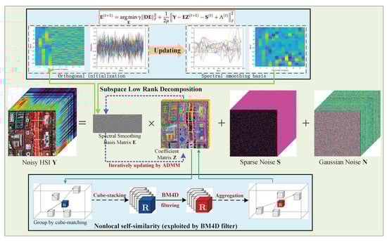
Figure 1.
Flowchart of the proposed SNSSLrL method.
The main contributions of this paper are summarized as follows.
- The sampled HSI is first projected into a low-dimensional subspace, which greatly alleviates the complexity of the denoising algorithm. Then, spectral smoothing regularization is enforced to the basis matrix of the subspace, which constrains the reconstructed HSI to maintain spectral smoothness and continuity.
- The plug-and-play non-local BM4D denoiser is enforced to the coefficient matrix of the subspace to fully utilize the self-similarity of the spatial dimension of HSI. Furthermore, the norm is used to separate the sparse noise. In the process of alternate optimization, the latent clean HSI is gradually learned from the degraded HSI.
The remainder of this paper is organized as follows. Section 2 formulates the preliminary problem of HSI mixed denoising and elaborates the proposed SNSSLrL model. In Section 3 and Section 4, experimental evaluations compared to the latest denoising methods are conducted to demonstrate the performance of our proposed SNSSLrL method. Eventually, the conclusion and future work are summarized in Section 5.
2. Materials and Methods
2.1. Degradation Model
In the complex process of signal acquisition and digital imaging, HSI is often contaminated by Gaussian noise and sparse noise. Gaussian noise refers to noise whose probability density obeys Gaussian distribution, e.g., dark noise and read noise. Sparse noise refers to a small proportion of noise in the sampled HSI, e.g., stripes, salt & pepper, deadlines, etc. According to the additive principle of noise, the denoising problem of an HSI with the size of can be formulated as:
where is the matrix formed by the vectorization of the third-order tensor , which is used to represent the degraded HSI (). is a latent clean image, is the Gaussian noise exist in HSI, and is the sparse noise, i.e., salt and pepper, stripes, and deadlines. Given the sampled image , clean can be restored by separating and .
Evidently, in Equation (1), cannot be solved directly from . Therefore, the priors of each component are required to compress the solution domain of the uncertain equation. Through the introduction of regularization constraints, the original additive model is transformed into the following regularization model:
where and are the regularization terms of clean HSI and sparse noise. The idea of regularization refers to introducing certain constraints by using the prior information of the image and noise to compressing the solution space of the uncertainty problem. describes the prior information of the latent noise-free image , such as low-rank property. describes the prior information of sparse noise to ensure that the observation image is decomposed into low-rank component and sparse noise without excessive deviation, such as the norm.
The low-rank regularization and non-local regularization of the latent clean HSI have been proven to achieve fine denoising results. Imposing the rank constraints on the potential clean image, low-rank regularization can separate the latent clean low-rank component from the full-rank noise component. As there are similar patches that exist in HSI, many denoising studies use non-local regularization to explore this self-similarity. For sparse noise , norm is able to fully use its sparse property. is a regularization parameter which is employed to control the contribution of different regularization terms. Fidelity term is used to constrain the Gaussian noise, where is the standard deviation of noise.
2.2. Subspace Low-Rank Regularization
Even working favorably on the HSI denoising problem, the following disadvantages still exist in above regularization model:
- If heavy Gaussian noise exists in the sampled image, it is difficult to obtain a fine denoising result by low-rank regularization. Meanwhile, since some sparse noises will also show a certain extent of low-rankness, low-rank regularization is also powerless in such a case.
- For the non-local regularization, the denoising result depends heavily on the choice of the search window and neighborhood window, and the cost of fine denoising results is often exchanged for greater execution time. In real scenarios, too much calculation time is often undesirable.
To address the above problems, we have developed the subspace low-rank learning methods in our previous work [2,19,59,60,61]. The principle of linear mixing in HSI instructs us that high-dimensional HSI exists in a subspace spanned by endmembers. Projecting the original high-dimensional image data into a low-dimensional subspace spanned by an orthogonal basis makes full use of the spectral low-rankness. Then imposing the non-local regularization constraints on the coefficient component of the subspace to realize the utility of the spatial self-similarity of HSI. Therefore, the subspace low-rank regularization model is formulated as
where is the basis of subspace and is the orthogonal constraint designed to drive spans more of the original space. is the low-rank regularization term imposed on coefficient of subspace instead of the original image. The function represents that a non-local transformation is performed on the coefficient to utilize the non-local self-similarity of the image. and is regularization parameters which are used to control the contribution of nuclear norm and sparse norm. The fidelity term indicates the subspace low-rank decomposition, i.e., .
In this way, the regularization operations imposed on the original high-dimensional image are transformed into the operations executed in the subspace. Not only enhances the exploration of low-rankness but also greatly reduces the computational complexity of the non-local algorithm.
2.3. Proposed Model
To further improve the performance of the subspace representation model, in this section, we proposed the spectral-smoothness regularized subspace low-rank learning model with non-local denoiser. Firstly, in our design, the original high-dimensional image data are projected into a low-rank subspace to obtain the basis matrix and coefficient matrix of the subspace. Then, spectral smoothing regularization is applied to the obtained basis matrix instead of orthogonal constraints. Meanwhile, the parameter-free non-local BM4D denoiser is embedded into the subspace model in a plug-and-play manner. Since the spectral continuous basis can promote the reconstruction of the continuous clean image data, and the non-local algorithm can remove the heavy Gaussian noise, the proposed model can achieve better restoration of the latent clean data. The proposed model is formulated as
where is the spectral smoothing term, is the first-order difference operator along the spectral dimension. For , the well-known plug-and-play parameter-free BM4D denoiser is employed. The idea of the BM4D denoising algorithm is to use the non-local self-similar property to achieve denoising. Because there are many similar non-local regions that exist in the natural image, BM4D extracts three-dimensional similar cubes from image tensor and stacks them to form a four-dimensional non-local tensor. Then the noise in the four-dimensional tensor is removed through the least square filtering [20]. In the process of solving, a spectral smoothing basis and a clean coefficient are learned. Our designed model not only inherited well the high computational efficiency of the subspace representation model but also further improved the accuracy of denoising. The embedding of parameter-free non-local BM4D denoiser also greatly reduces the parameter complexity of the model, which is very critical in practical applications.
2.4. Optimization
It is extremely difficult to solve Equation (4) directly. Here we design an optimization approach to solve the proposed SNSSLrL model. Through introducing a Lagrangian multiplier , the original model is transformed into the following Lagrangian equation:
where is the penalty parameter, is a Lagrangian multiplier. The above Lagrangian equation can be solved by alternate iteration [62]. In each iteration, fixing the remaining variables and only updating the current variable, the optimization of Equation (5) can be transformed into the optimization of the following three subproblems. Through alternate updating, the basis and coefficient of the subspace are learned iteratively, thus realizing the reconstruction of potentially latent data. The main steps of solving Equation (5) are summarized in Algorithm 1.
| Algorithm 1 Optimization procedure for solving Model 4. |
| Require: The degraded HSI , stop criterion , regularization parameters and , |
| maximum iteration , dimension of subspace k. |
| Ensure: The latent noise-free data . |
| 1: Initialization: Estimate via SVD, set , set . |
| 2: while not converged do |
| 3: Update by Equation (7). |
| 4: Update by Equation (10). |
| 5: Update by Equation (12). |
| 6: Update by Equation (13). |
| 7: Update iteration by |
| 8: end while |
| 9: return . |
- Update (Line 3): The subproblem of updating is given by:which can be solved by the parameter-free plug-and-play BM4D denoiser:
- Update (Line 4): The subproblem of updating is given by:which can be transformed into solving the following Sylvester equation:where is a circulant matrix, is a symmetric matrix. Therefore, by using first-order Fourier transform to diagonalize and first-order SVD to diagonalize , that is and , a closed-form solution of Equation (7) is obtained bywhere .
- Update (Line 5): The subproblem of updating is given by:Here we use the soft-thresholding function to solve this subproblem efficiently:where is the thresholding parameter. is the absolute operation of matrix .
- Update (Line 6): Updating Lagrangian multiplier is given by:
3. Results
3.1. Simulation Configurations
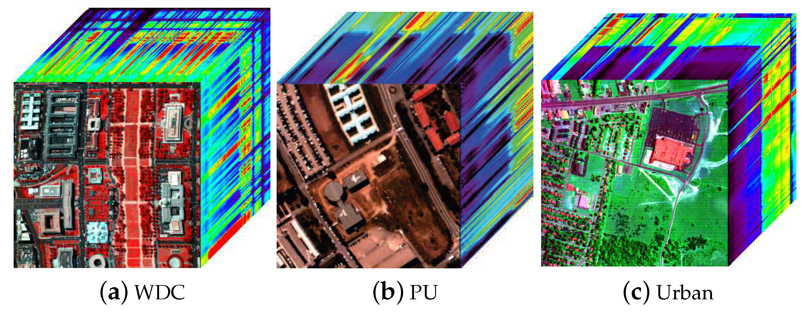
As shown in Figure 2, two datasets were used in the simulated numeric experiments, i.e., HYDICE Washington DC Mall (WDC), ROSIS Pavia University (PU) and HYDICE Urban. They have 191 and 103 high-quality spectral bands, respectively. Sub-images with the spatial size of 256 × 256 are cropped for simulation. The well-known HYDICE Urban dataset whose size is 307 × 307× 210 is used for the real experiment. Many bands of Urban dataset are severely degraded by watervapour absorption and mixed noise. To verify the denoising performance of the proposed algorithm, six representative state-of-the-art HSI denoising methods are used as competitors, i.e., SLRL4D [61], 3DlogTNN [58], LRTDGS [63], LRTDTV [55], LLRSSTV [64], FSSLRL [60]. Among them, SLRL4D and FSSLRL are subspace-based methods, 3DlogTNN, LRTDTV, and LRTDGS are the latest tensor representation-based methods. All experiments are conducted on a workstation with dual Intel Silver 4210 and 128 G of RAM.
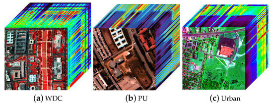
Figure 2.
Falsecolor maps of the simulated and real HSI datasets.
To quantitatively assess the performance of denoisers, indexes such as peak-signal-to-noise-ratio (PSNR), structural similarity (SSIM), feature similarity index mersure (FSIM), Erreur relative global adimensionnelle de synthèse (ERGAS), and mean spectral angle (MSA) are used in the subsequent four cases of simulation.
- case 1: zero-mean Gaussian noise with the randomly selected variance in the range from 0.2 to 0.25 is first added to all bands. Meanwhile, in 20 continuous bands, 10% of pixels are contaminated by salt and pepper noise.
- case 2: zero-mean Gaussian noise is added as the same condition in case 1, and deadlines with the randomly selected number in the range [3, 10] and widths in [1, 3] are added to the continuous 20 bands.
- case 3: zero-mean Gaussian noise is added as the same condition in case 1, and stripes with the randomly selected number in the range [2, 8] are added to the continuous 20 bands.
- case 4: Simultaneously add all the noises in cases 1–3 to simulate mixed noise.
3.2. Experimental Results on Simulated Datasets
3.2.1. Parameter Settings for Simulated Datasets
In order to reproduce the results of algorithms in this article for other interested readers, Table 1 shows the parameter settings of all the comparison methods on the simulated datasets. The parameters of the comparison methods are first set to the recommended parameter settings in the corresponding references and then those values associated to the optimal results for each dataset are adopted after fine-tuning.

Table 1.
Parameter settings for all competing algorithms in both simulated and real datasets.
3.2.2. Visual Evaluation Results
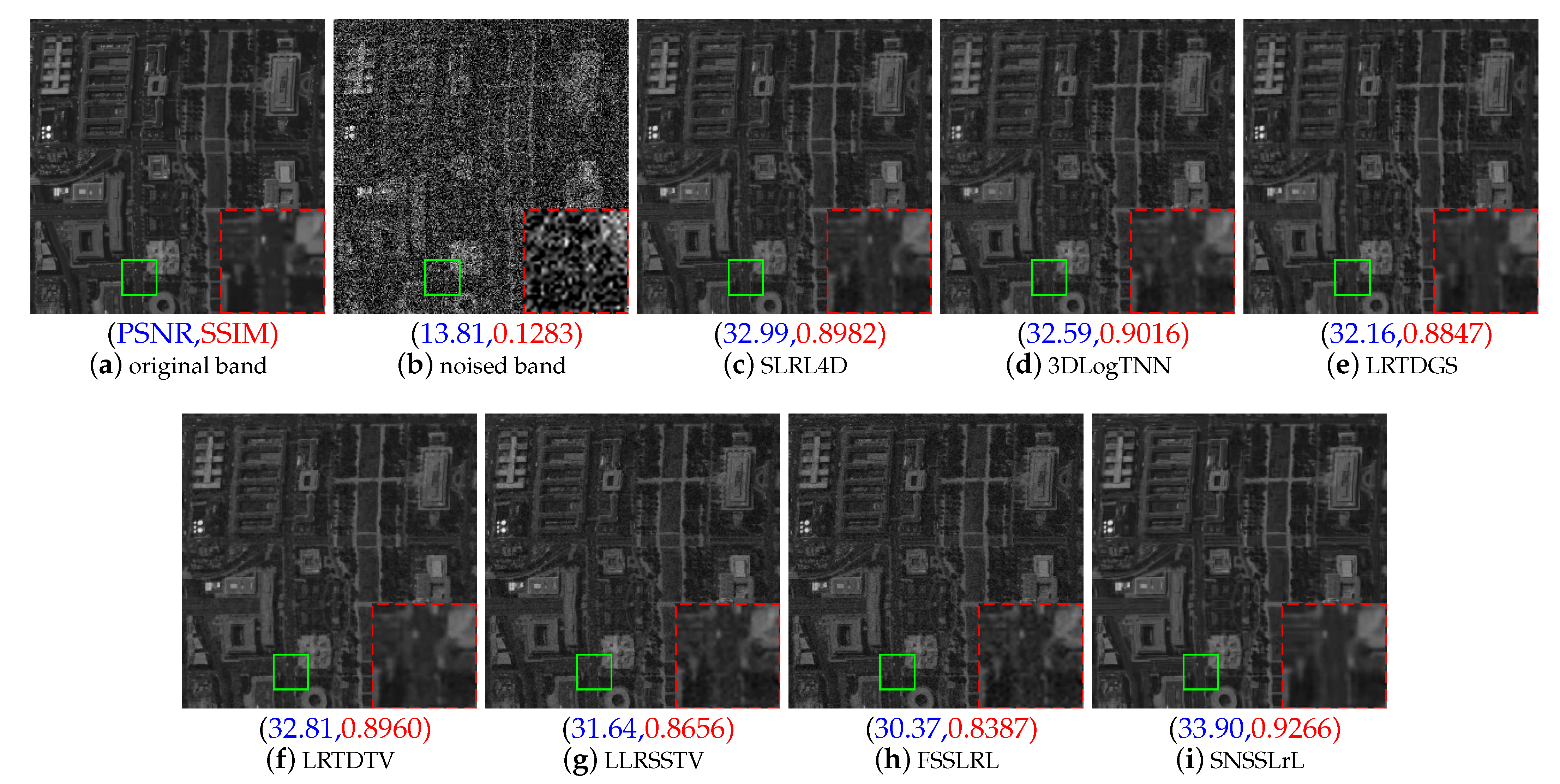
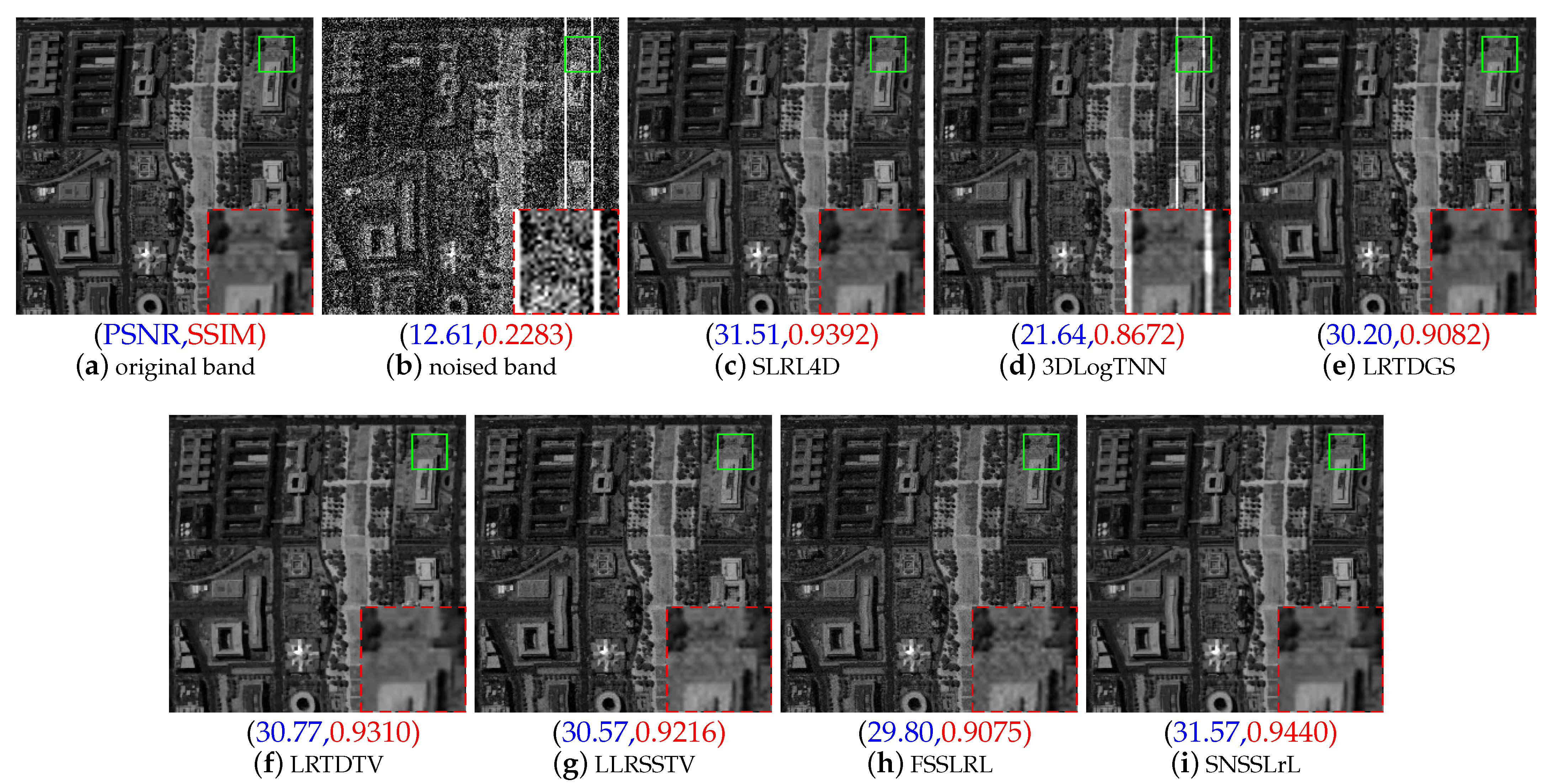
Among the four different cases, we chose representative case 1 and case 4 to evaluate the visual effects of seven different methods. Figure 3 and Figure 4 show the recovery of the WDC data set. Figure 5 and Figure 6 illustrate the recovery of the PU data set.
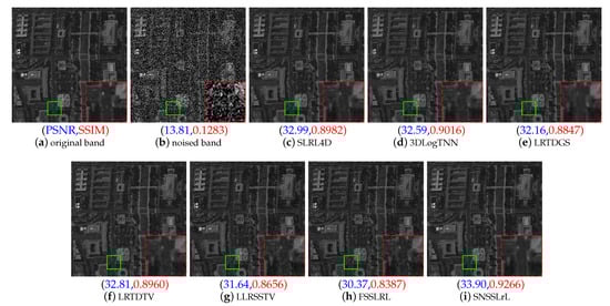
Figure 3.
Band image on spectral band 28 of WDC dataset under simulated case 1. (a) Original band; (b) Noised band; (c) SLRL4D; (d) 3DLogTNN; (e) LRTDGS; (f) LRTDTV; (g) LLRSSTV; (h) FSSLRL; (i) SNSSLrL.
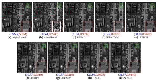
Figure 4.
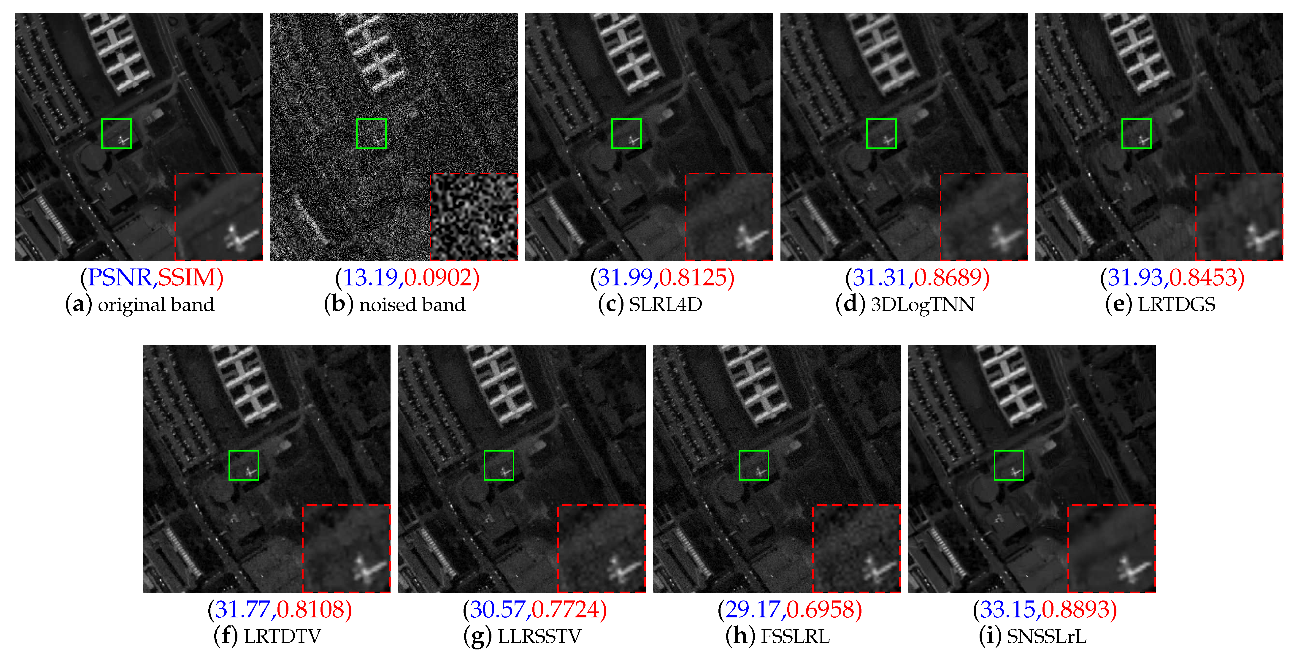
Band image on spectral band 117 of WDC dataset under simulated case 4. (a) Original band; (b) Noised band; (c) SLRL4D; (d) 3DLogTNN; (e) LRTDGS; (f) LRTDTV; (g) LLRSSTV; (h) FSSLRL; (i) SNSSLrL.
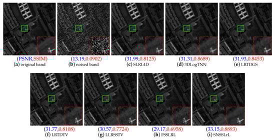
Figure 5.
Band image on spectral band 23 of PU dataset under simulated Case 1. (a) Original band; (b) Noised band; (c) SLRL4D; (d) 3DLogTNN; (e) LRTDGS; (f) LRTDTV; (g) LLRSSTV; (h) FSSLRL; (i) SNSSLrL.
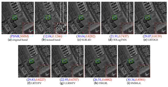
Figure 6.
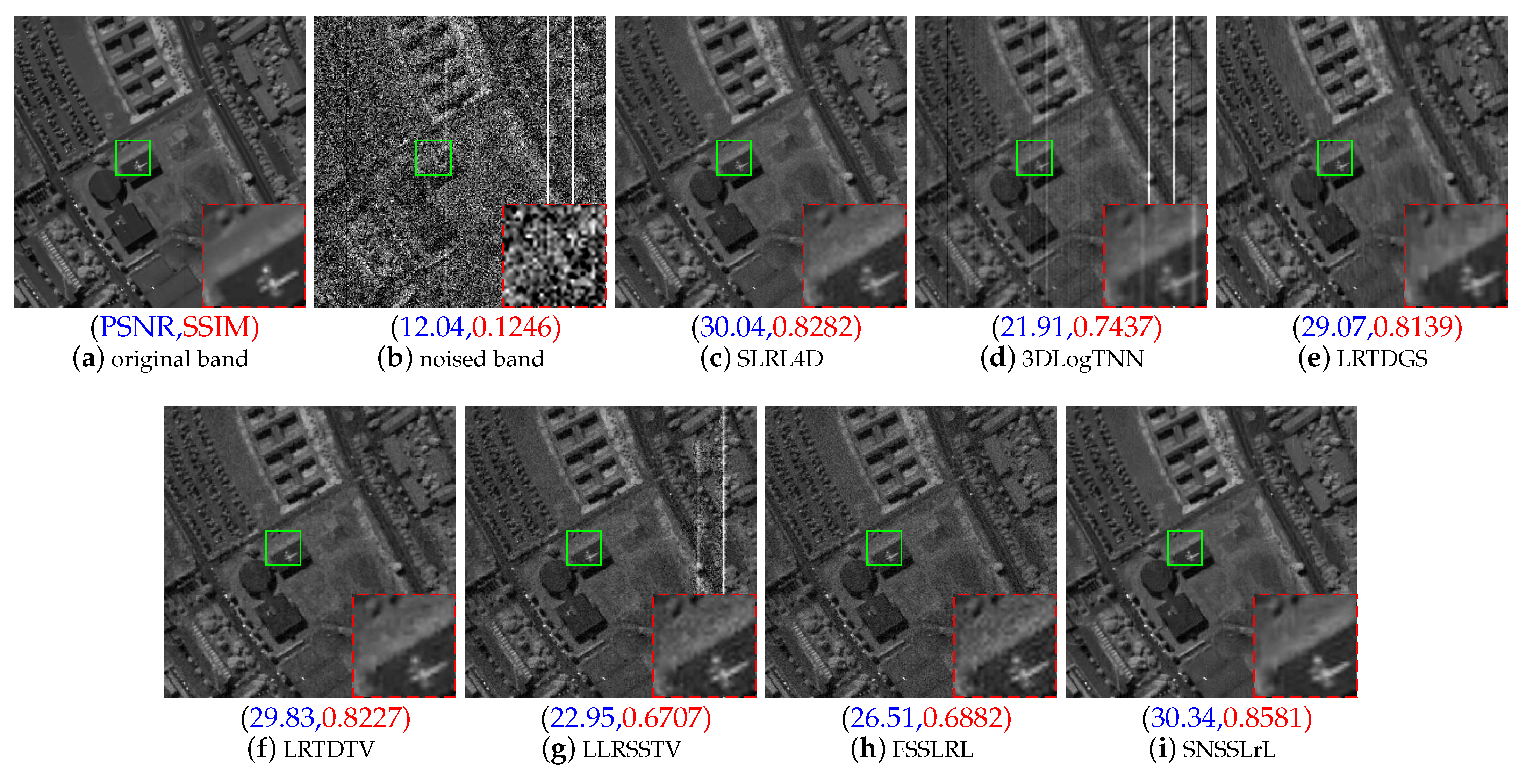
Band image on spectral band 82 of PU dataset under simulated Case 4. (a) Original band (b) Noised band (c) SLRL4D (d) 3DLogTNN (e) LRTDGS (f) LRTDTV (g) LLRSSTV (h) FSSLRL (i) SNSSLrL.
Figure 4b shows that severe mixed noise (impulse noise, stripes, and deadlines) destroys the high-frequency information of band 105 of the WDC under case 4, and the ground information is almost in an invisible state. It is clear that the FSSLRL method and the LLRSSTV method do not completely deal with the impulse noise, the image restored by the LRTDGS method is blurred, that is, a lot of detailed image information is lost. The 3DlogTNN method cannot complete the task of removing noise at edges. The denoising effect of the LRTDTV method and the SLRL4D method is superior to other methods, but compared with our SNSSLrL method, both in the smoothness of image restoration and detail preservation, there are obvious shortcomings. In Figure 3, we can get similar conclusions, where the 3DlogTNN method does not have the processing task of fringe noise in case 1, but its processing effect is still not ideal, mainly reflected in the loss of details. Although 3DlogTNN considers the third-order tensor of HSI, that is, considering both spatial and spectral information, it is only designed to remove Gaussian noise. Therefore, it appears powerless for removing the complex mixed noise in HSI. Due to the lack of spatial constraints, the FSSLRL achieves the lowest PSNR value. Unsurprisingly, among all the comparison methods, the proposed SNSSLrL denoiser achieves the best denoising effect. Figure 3 shows the PSNR and SSIM values of all methods on band 28 of the WDC dataset.
Figure 5 shows that in the PU dataset, without stripes or bad lines, the recovery effect of the FSSLRL, LRTDGS, and LLRSSTV methods is obviously not as good as the other four methods. Meanwhile, 3DLogTNN, LRTDGS, and SLRL4D are obviously not as good as our SNSSLrL method. Compared with the second-placed SLRL4D method, the proposed SNSSLrL method achieves 1.16 dB and 0.0768 higher on PSNR and SSIM, respectively. The performance of each algorithm in the PU dataset in removing mixed noise is similar to their performance in the WDC dataset. It is clear that Figure 6b shows that band 82 of the PU dataset has been added with strong impulse noise, stripes, and deadlines. Both 3DLogTNN and LLRSSTV methods failed to effectively remove the stripes and deadlines. Although FSSLRL, LRTDGS, and LRTDTV can remove all the stripes and deadlines, they have poor performance in maintaining the details of the image. The PSNR values obtained by them are 26.51, 29.07, and 29.83 dB, respectively. The SLRL4D method and the proposed SNSSLrL method have achieved better mixed noise removal effects, but SNSSLrL is better in maintaining image details, especially the edge details of geometric shapes in the red box.
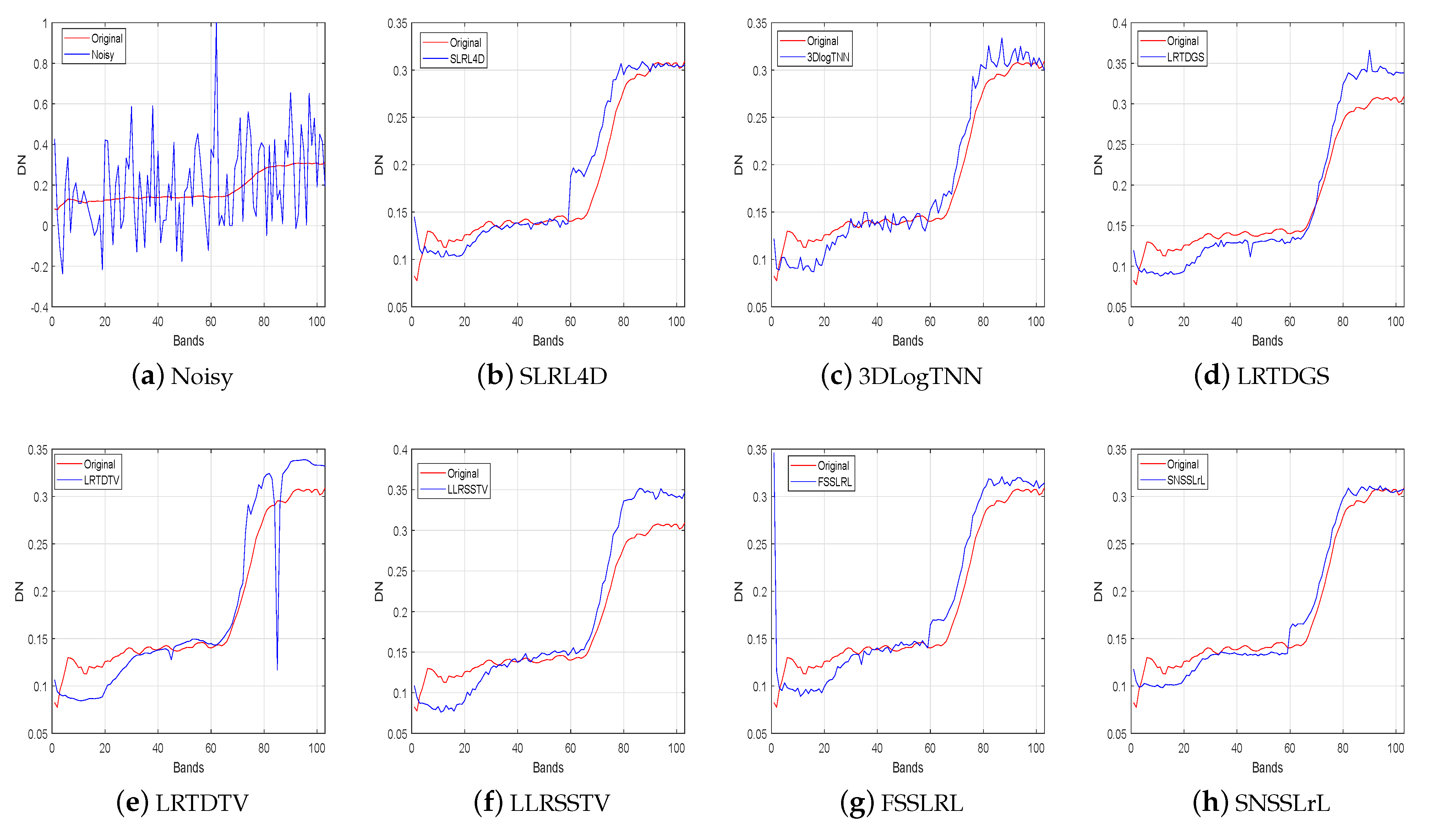
To further compare the performance of each algorithm, Figure 7 shows the spectral curve reconstructed by each algorithm at pixel (100,100) in case 4 of the PU dataset, where the red curve represents the true spectrum, and the blue curve represents the reconstructed one. It is clear that the LRTDTV method fails to effectively reconstruct the corresponding spectrum. The spectrum reconstructed by 3DLogTNN contains a lot of violent fluctuations, indicating that its performance is unstable on more bands, and there are still some noises that have not been removed. For LRTDGS, LLRSSTV, and FSSLRL methods, their reconstruction accuracy on the 1–10 band and 80–100 band is much lower than the proposed SNSSLrL method. For the SLRL4D method, its reconstruction accuracy in the 60–70 band is lower than the proposed method. Therefore, benefiting from the spectral smoothing constraint on the subspace basis, the proposed SNSSLrL method achieves the closest reconstruction to the true spectrum.
Figure 7.
The compsarison of the reconstructed spectrum by different method at pixel (100, 100) in case 4 of PU dataset.
3.2.3. Quantitative Evaluation Results
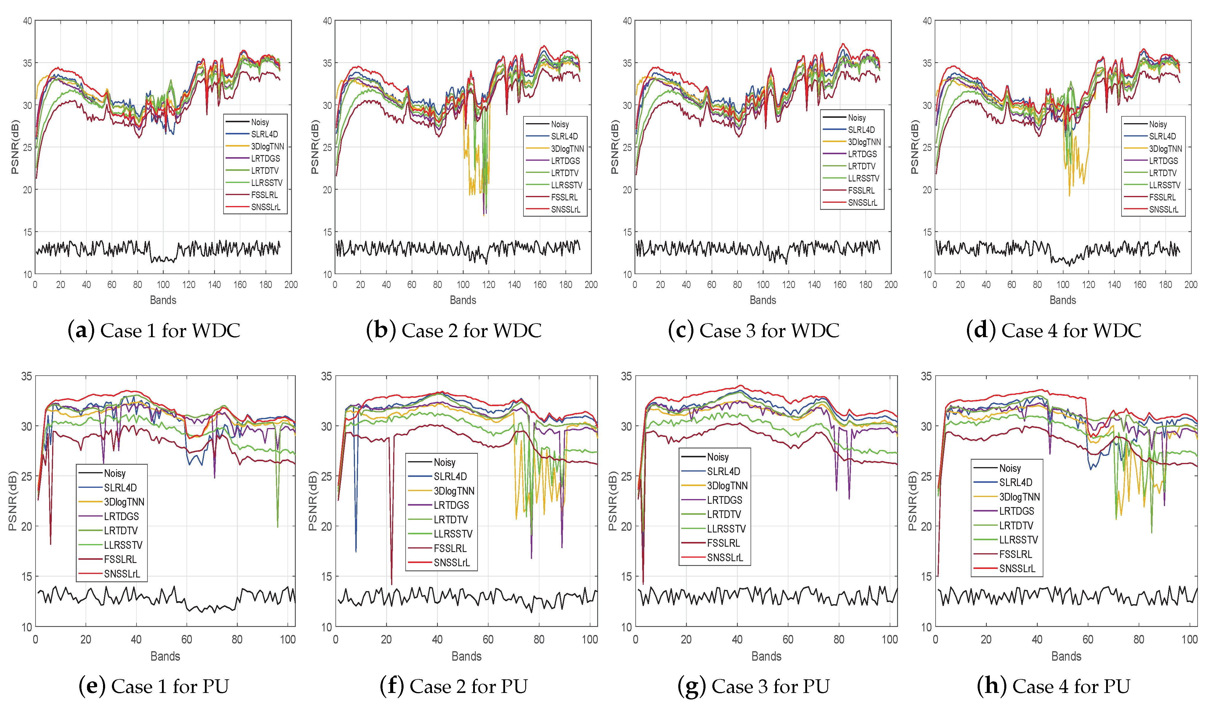
To quantitatively evaluate the performance of each algorithm and give the reader a quantitative reference, Figure 8 shows the PSNR values as a function of bands for each algorithm under the four cases of WDC and PU datasets. In the first row of Figure 8, it is evident that the proposed SNSSLrL method is relatively stable in removing Gaussian noise and impulse noise. Its performance on the band 1–60 and 120–188 exceeds all comparison algorithms, but on the 60–120 band, the performance is relatively ordinary. Meanwhile, for mixed noise, especially stripes and deadlines (as shown in Figure 8b,d), although the proposed method does not achieve the best results on all bands, its stability and average performance is the best. The reason is that the subspace decomposition can effectively suppress the influence of noise, furthermore, the spectral smoothing constraint on the subspace basis enables the reconstructed image to maintain a certain continuity between the upper and lower bands, thereby further maintaining image details. In the second row of Figure 8, it is clear that the proposed method has achieved the best PSNR values on almost all bands, which shows that for PU data, whether it is Gaussian noise, impulse noise, or mixed noises, the proposed SNSSLrL method can achieve a better denoising performance than the other six competitors.
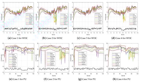
Figure 8.
MPSNR as a function of bands for case 1 to case 4 of WDC and PU datasets.
Table 2 lists the quantitative denoising results of the above seven algorithms in four cases on the WDC and PU datasets, with a total of five indicators. For case 1 of WDC, the PSNR value of SNSSLrL is 0.03 dB higher than the second-place 3DLogTNN method, while the ERGAS value is 0.69 higher (the lower the ERGAS value, the better the algorithm performance). For the other cases of the two datasets, the proposed SNSSLrL method has achieved the best quantitative results on the five indicators. For example, for case 4 of PU data, the proposed SNSSLrL method achieves a PSNR value of 0.78 dB higher than the second place LRTDTV method.
Table 2.
Quantitative results under all four different simulated case (the optial results are highlighted in bold).
In conclusion, whether it is simple Gaussian noise and impulse noise or complex mixed noise, the proposed SNSSLrL method achieves the best results in all terms of visual effects and quantitative evaluation of HSI recovery compared to all six competitors.
3.2.4. Visual Evaluation Results
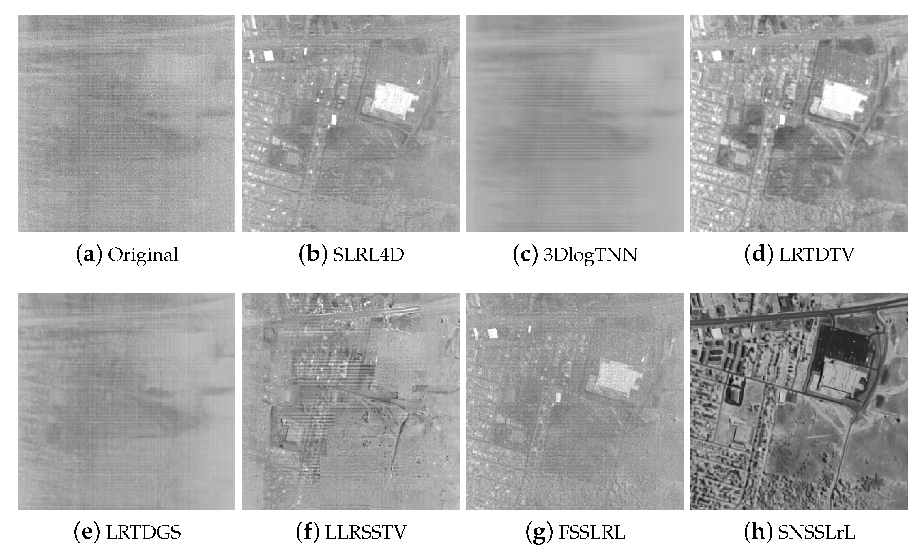
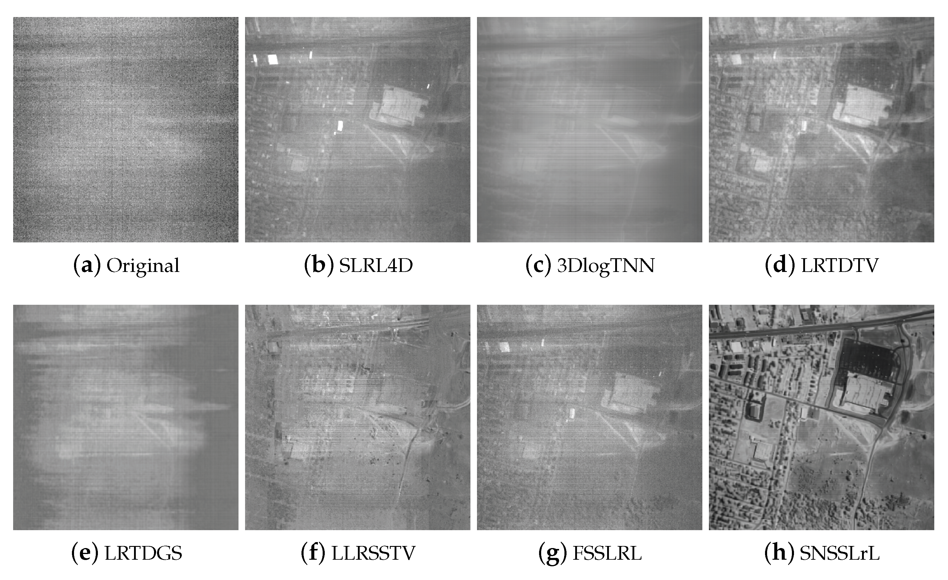
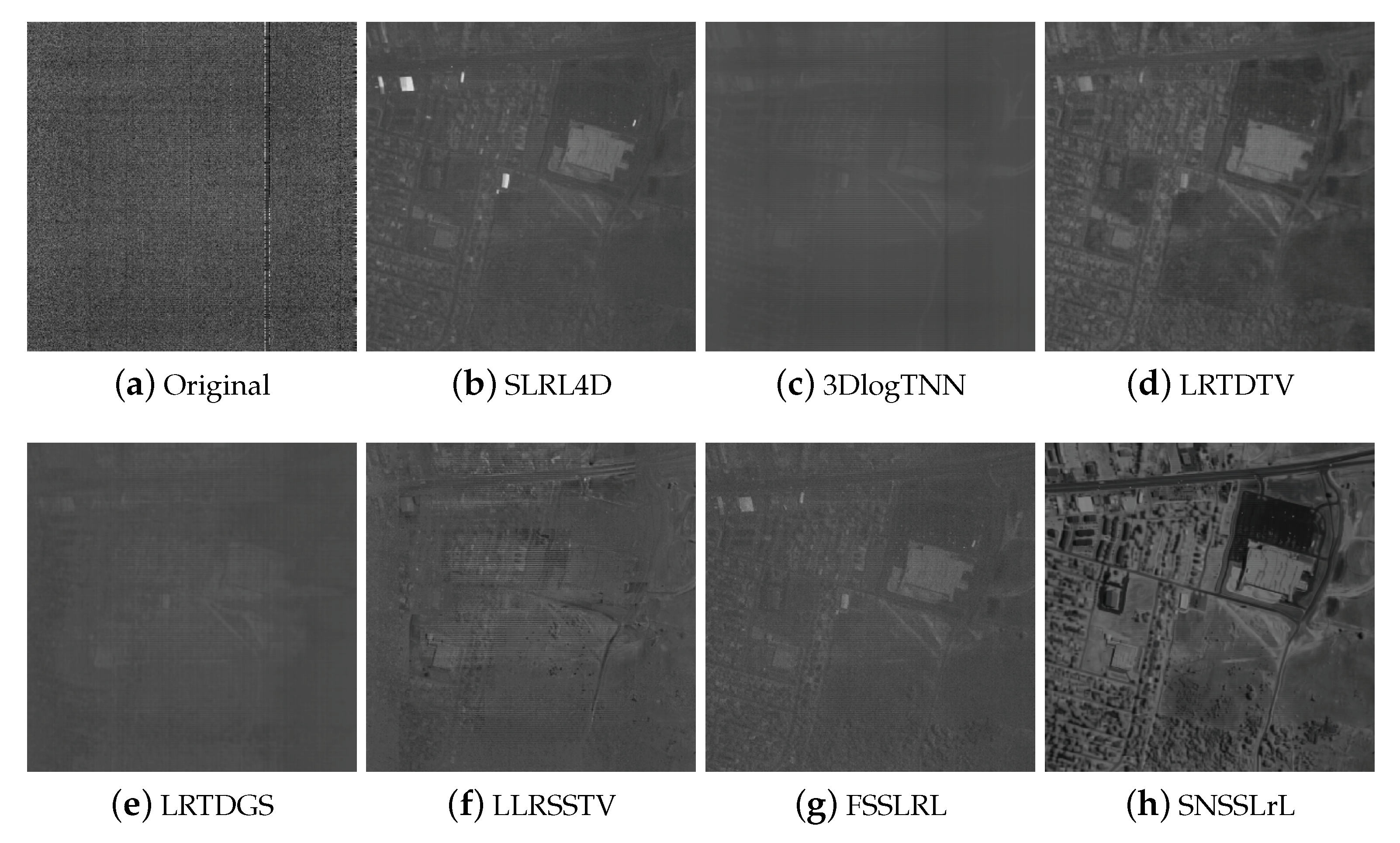
Figure 9, Figure 10 and Figure 11 illustrate the denoising results of the above algorithms on the 105, 144, and 211 bands of the real hyperspectral dataset—the HYDICE Urban. About 20 bands in this image are affected by severe mixed noise, for instance, band 105 (as shown in Figure 9a) contains severe Gaussian noise, impulse noise, and vertical stripe noise; band 144 (as shown in Figure 10a) contains severe Gaussian noise, impulse noise, and horizontal stripe noise; band 210 (as shown in Figure 11a) is one of the most severely contaminated bands by noise, and it is almost impossible to see that it contains any useful information. From the reconstruction results in the above figure, it can be seen that the 3DLogTNN, LRTDGS, and LLRSSTV methods failed to restore the 105, 144, and 210 bands and most of the information of the reconstructed image has been lost. Thanks to the subspace decomposition framework and the spatial-spectral total variation constraint, the SLRL4D, FSSLRL, and LRTDTV methods can recover part of the image information, but most of the details are lost. For the above three severely polluted bands, only the proposed method reconstructed satisfactory results, which contain many fine details in the image.
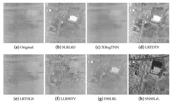
Figure 9.
Real comparison of all methods on bands 105 of Urban dataset.
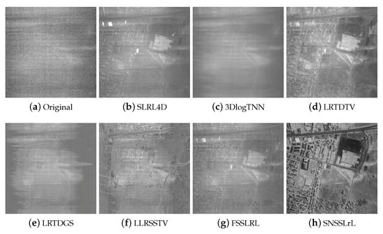
Figure 10.
Real comparison of all methods on bands 144 of Urban dataset.
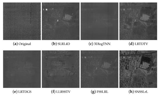
Figure 11.
Real comparison of all methods on bands 210 of Urban dataset.
3.3. Experimental Results on Real Datasets
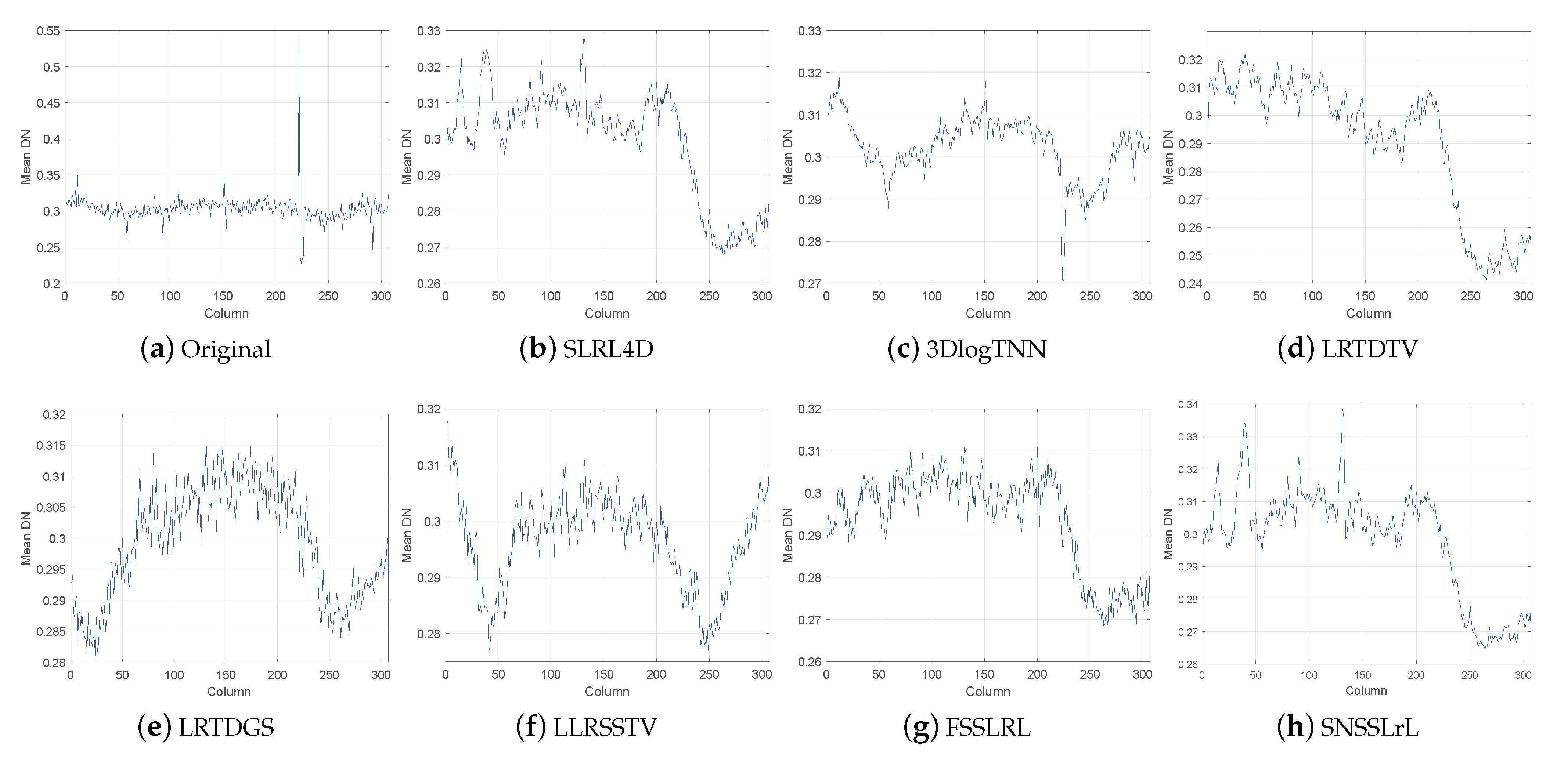
Figure 12 plots the horizontal mean profiles of band 210 of the urban dataset. The horizontal mean profile can effectively reflect the mixed noise in the image, especially the impulse noise and band noise. As shown in Figure 12a, due to the pollution of heavy mixed noise in band 210, the horizontal mean profile of the original band 210 fluctuates rapidly. From Figure 12, the following conclusions can be drawn: The horizontal mean profiles of the LRTDGS, LLRSSTV, and FSSLRL methods contain higher-frequency fluctuations, indicating that the serious stripe noise has not been removed. Compared with SLRL4D, LRTDTV, and the proposed SNSSLrL method, the horizontal mean profile of 3DLogTNN is significantly different. The reason may be that due to the serious mixed noise pollution on the continuous bands, the 3DlogTNN method cannot effectively use the inter-band information to reconstruct the image. Compared with these methods, our proposed SNSSLrL achieves a flatter curve, which indicates that the cross stripes and various other noises of the urban data set are more effectively eliminated.
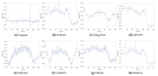
Figure 12.
The comparison of the horizontal mean profiles of band 210 of the constructed urban dataset by different denoising methods.
In summary, the competitive recovery results of our proposed SNSSLrL denoiser have been verified.
Quantitative Evaluation Results
To further verify the effectiveness of the SNSSLrL in real scenarios, Q-metric was used to quantitatively evaluate the denoising effect of each algorithm on urban data. Q-metric is a blind image spatial information index [65]. The greater value of Q-metric represents a better preservation of spatial details in the image. Table 3 lists the average Q-metrics of all bands in the urban dataset, the optimal is bolded. It is evident that the proposed SNSSLrL denoiser obtains the highest Q value, which indicates that it delivers the best restoration results in preserving the spatial fine details compared to the other six denoisers.
Table 3.
Q-metric of the reconstructed results of the competing methods on urban dataset.
The running time of an algorithm is one of the important indicators used to measure the possibility of the real application of the algorithm. Table 4 lists the execution time of all competing methods on the real urban dataset, the optimal is bolded. The results in Table 4 are the average of ten running times, and all algorithms are performed in the same experimental environment. As shown in the table, the subspace decomposition techniques, such as FSSLRL, SLRL4D, and the proposed SNSSLrL method, have outstanding performance in computational efficiency and take less time than the other four methods. Thanks to the spectral smoothing constraint on subspace basis, SNSSLrL achieves better denoising effects with fewer iterations, which further saves running time.
Table 4.
Execution time (seconds) comparison of the competing methods on urban dataset.
4. Discussion
In the proposed SNSSLrL model, there are four important parameters, that is, dimension of subspace p, regularization parameters and , and the Lagrangian parameter . Since BM4D denoiser is a parameterless method, we do not need to make strict parameter adjustments for the non-local item in the model.
4.1. The Regularization Parameters , and
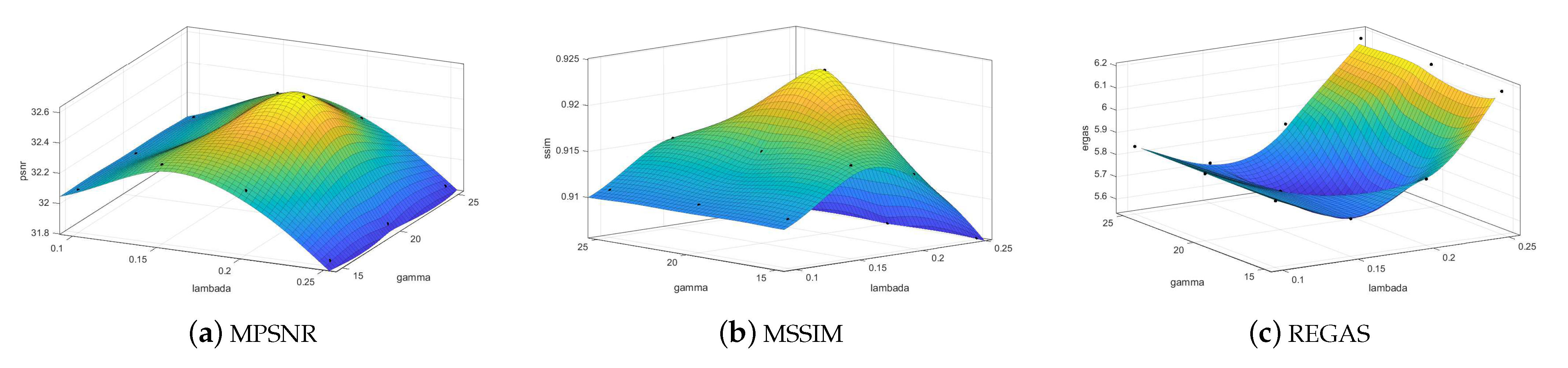
As shown in Formula (5), is a Lagrangian parameter. In theory, when tends to positive infinity, Formula (5) has the same solution as model (4). However, in actual applications, we usually set to get a good result. The regularization parameters and indeed have a great impact on the experimental results. Figure 13 shows the sensitivity analysis of the parameters and in case 4 of the simulated WDC dataset. It can be seen that when is located in the interval of [15–25] and is located in the interval of [0.1–0.2], the proposed SNSSLrL algorithm can achieve a relatively stable and satisfactory result on PSNR, SSIM, and ERGAS indicators, respectively.

Figure 13.
In case 4 of the simulated WDC dataset, the sensitivity analysis of the parameters and is carried out by using the MPSNR, MSSIM, and ERGAS.
4.2. The Dimension of Subspace p
The parameter p is an important parameter related to the subspace dimension. According to the linear mixing theory, its ideal value should be equal to the number of end-members existing in the scene. However, in actual scenarios, due to the complex nonlinear mixture, the ideal value of parameter p is difficult to guarantee. Therefore, in our experiments, the value of p is fixed to 4. we suggest choosing the optimal value of p in the range of [3–8].
4.3. Convergence Analysis
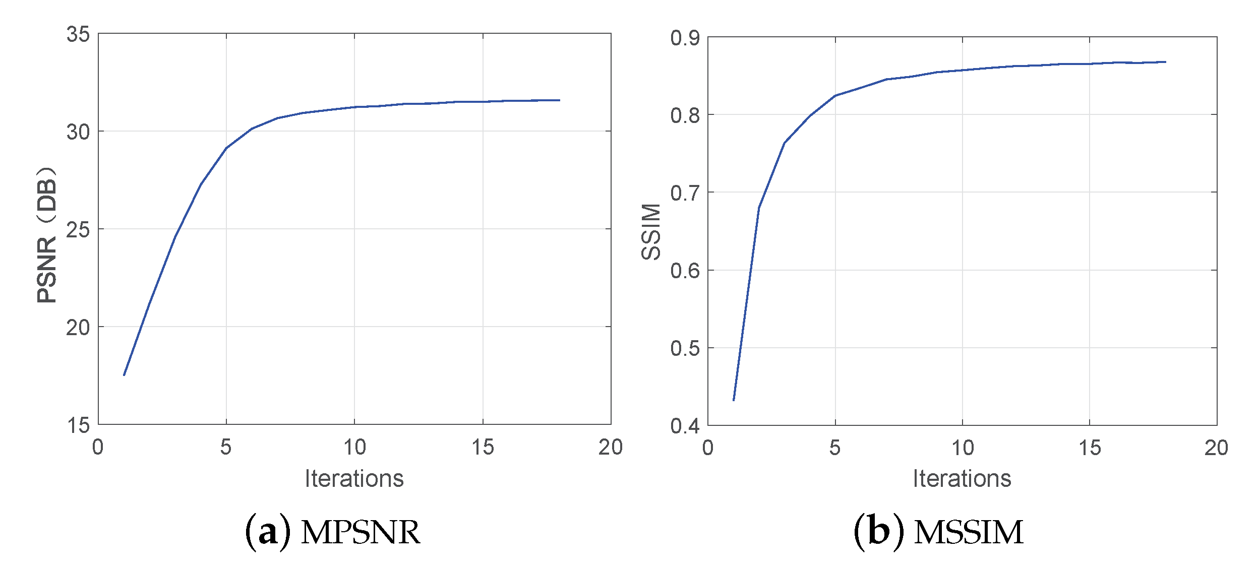
Figure 14 plots the MPSNR and MSSIM values as a function of iterations under case 2 of the simulated PU dataset. It is clear that both the MPSNR value and the MSSIM value quickly enter a stable state after the first few iterations, which demonstrates that the proposed SNSSLrL algorithm has good convergence.
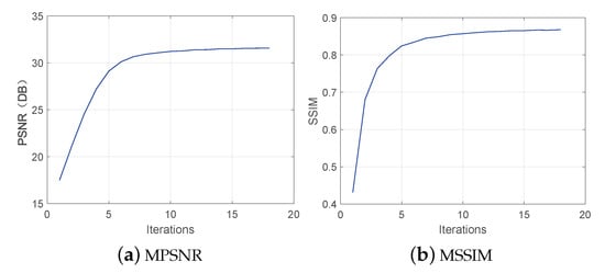
Figure 14.
The MPSNR and MSSIM values as a function of iterations in case 2 of the simulated PU dataset.
5. Conclusions and Future Work
In the framework of subspace decomposition, in the paper, a mixed noise removal algorithm is proposed for HSI that uses both spectral smoothing prior and non-local self-similar prior. The proposed SNSSLrL model was solved quickly and efficiently by the ADMM algorithm. Experiments on two simulated datasets and a real dataset show that the proposed spectral smoothing constraint on the subspace basis can effectively characterize the intrinsic properties of the subspace, and further improve the effect of mixed denoising. All indicators surpass several state-of-the-art HSI denoising algorithms with high time efficiency.
Future work will focus on utilizing advanced technology to exploit non-local similarities under the framework of subspace decomposition, and perform subspace decomposition in the sense of tensors, to achieve more accurate spatial-spectral information mining, thereby further improving the efficiency and accuracy of mixed noise removal.
Author Contributions
Conceptualization, C.H.; funding acquisition, L.S. and C.H.; investigation, W.L.; methodology, L.S. and C.H.; software, W.L.; supervision, L.S.; validation, W.L.; visualization, L.S. and W.L.; writing—original draft, L.S., C.H. and W.L. All authors have read and agreed to the published version of the manuscript.
Funding
This study was supported by the National Natural Science Foundation of China [61971233, 62076137, U1831127], the Henan Key Laboratory of Food Safety Data Intelligence [KF2020ZD01], and the Postgraduate Research & Practice Innovation Program of Jiangsu Province [KYCX21_1004].
Institutional Review Board Statement
Not applicable.
Informed Consent Statement
Not applicable.
Data Availability Statement
Not applicable.
Conflicts of Interest
The authors declare no conflict of interest.
Abbreviations
The following abbreviations are used in this manuscript:
| HSI | Hyperspectral image |
| ADMM | Alternating Direction Method of Multipliers |
| BM4D | Block-Matching and 4D filtering |
| PCA | principal component analysis |
| LRMR | low-rank matrix restoration |
| CP | CANDECOMP/PARAFAC |
| CNN | convolutional neural network |
| TV | Total variation |
| WDC | Washington DCMall |
| PU | Pavia University |
| PSNR | Peak-Signal-to-Noise Ratio |
| SSIM | Structural Similarity Index Mersure |
| FSIM | Feature Similarity Index Mersure |
| ERGAS | Erreur Relative Global Adimensionnelle de Synthèse |
| MSA | Mean Spectral Angle |
References
- Wu, Z.; Sun, J.; Zhang, Y.; Wei, Z.; Chanussot, J. Recent Developments in Parallel and Distributed Computing for Remotely Sensed Big Data Processing. Proc. IEEE 2021. [Google Scholar] [CrossRef]
- He, C.; Sun, L.; Huang, W.; Zhang, J.; Zheng, Y.; Jeon, B. TSLRLN: Tensor subspace low-rank learning with non-local prior for hyperspectral image mixed denoising. Signal Process. 2021, 184, 108060. [Google Scholar] [CrossRef]
- Sun, L.; Wu, F.; Zhan, T.; Liu, W.; Wang, J.; Jeon, B. Weighted nonlocal low-rank tensor decomposition method for sparse unmixing of hyperspectral images. IEEE J. Sel. Top. Appl. Earth Obs. Remote Sens. 2020, 13, 1174–1188. [Google Scholar] [CrossRef]
- Sun, L.; Wu, F.; He, C.; Zhan, T.; Liu, W.; Zhang, D. Weighted Collaborative Sparse and L1/2 Low-Rank Regularizations With Superpixel Segmentation for Hyperspectral Unmixing. IEEE Geosci. Remote Sens. Lett. 2020. [Google Scholar] [CrossRef]
- Lu, Z.; Xu, B.; Sun, L.; Zhan, T.; Tang, S. 3-D Channel and spatial attention based multiscale spatial–spectral residual network for hyperspectral image classification. IEEE J. Sel. Top. Appl. Earth Obs. Remote Sens. 2020, 13, 4311–4324. [Google Scholar] [CrossRef]
- Wang, J.; Song, X.; Sun, L.; Huang, W.; Wang, J. A novel cubic convolutional neural network for hyperspectral image classification. IEEE J. Sel. Top. Appl. Earth Obs. Remote Sens. 2020, 13, 4133–4148. [Google Scholar] [CrossRef]
- Pan, L.; He, C.; Xiang, Y.; Sun, L. Multiscale Adjacent Superpixel-Based Extended Multi-Attribute Profiles Embedded Multiple Kernel Learning Method for Hyperspectral Classification. Remote Sens. 2021, 13, 50. [Google Scholar] [CrossRef]
- Xu, Y.; Wu, Z.; Chanussot, J.; Wei, Z. Nonlocal patch tensor sparse representation for hyperspectral image super-resolution. IEEE Trans. Image Process. 2019, 28, 3034–3047. [Google Scholar] [CrossRef] [PubMed]
- Xu, Y.; Wu, Z.; Xiao, F.; Zhan, T.; Wei, Z. A target detection method based on low-rank regularized least squares model for hyperspectral images. IEEE Geosci. Remote Sens. Lett. 2016, 13, 1129–1133. [Google Scholar] [CrossRef]
- Hou, Y.; Zhu, W.; Wang, E. Hyperspectral mineral target detection based on density peak. Intell. Autom. Soft Comput. 2019, 25, 805–814. [Google Scholar] [CrossRef]
- Sun, L.; Zhan, T.; Wu, Z.; Jeon, B. A novel 3d anisotropic total variation regularized low rank method for hyperspectral image mixed denoising. ISPRS Int. J. Geo-Inf. 2018, 7, 412. [Google Scholar] [CrossRef] [Green Version]
- Elad, M.; Aharon, M. Image denoising via sparse and redundant representations over learned dictionaries. IEEE Trans. Image Process. 2006, 15, 3736–3745. [Google Scholar] [CrossRef] [PubMed]
- Buades, A.; Coll, B.; Morel, J. A non-local algorithm for image denoising. In Proceedings of the 2005 IEEE Computer Society Conference on Computer Vision and Pattern Recognition (CVPR’05), San Diego, CA, USA, 20–25 June 2005; Volume 2, pp. 60–65. [Google Scholar]
- Dabov, K.; Foi, A.; Katkovnik, V.; Egiazarian, K. Image denoising by sparse 3-D transform-domain collaborative filtering. IEEE Trans. Image Process. 2007, 16, 2080–2095. [Google Scholar] [CrossRef]
- Gu, S.; Lei, Z.; Zuo, W.; Feng, X. Weighted nuclear norm minimization with application to image denoising. In Proceedings of the 2014 IEEE Conference on Computer Vision and Pattern Recognition (CVPR), Columbus, OH, USA, 23–28 June 2014; pp. 2862–2869. [Google Scholar]
- Starck, J.L.; Candès, E.; Donoho, D.L. The curvelet transform for image denoising. IEEE Trans. Image Process. 2002, 11, 670–684. [Google Scholar] [CrossRef] [PubMed] [Green Version]
- Kopsinis, Y.; Mclaughlin, S. Development of EMD-based denoising methods inspired by wavelet thresholding. IEEE Trans. Signal Process. 2009, 57, 1351–1362. [Google Scholar] [CrossRef]
- Chen, G.; Qian, S. Denoising of hyperspectral imagery using principal component analysis and wavelet shrinkage. IEEE Trans. Geosci. Remote Sens. 2011, 49, 973–980. [Google Scholar] [CrossRef]
- Sun, L.; Jeon, B. Hyperspectral Mixed Denoising Via Subspace Low Rank Learning and BM4D Filtering. In Proceedings of the IGARSS 2018–2018 IEEE International Geoscience and Remote Sensing Symposium, Valencia, Spain, 22–27 July 2018; pp. 8034–8037. [Google Scholar]
- Maggioni, M.; Katkovnik, V.; Egiazarian, K.; Foi, A. Nonlocal transform-domain filter for volumetric data denoising and reconstruction. IEEE Trans. Image Process. 2013, 22, 119–133. [Google Scholar] [CrossRef] [PubMed]
- Wen, Y.; Ng, M.K.; Huang, Y. Efficient total variation minimization methods for color image restoration. IEEE Trans. Image Process. 2008, 17, 2081–2088. [Google Scholar] [CrossRef]
- Yuan, Q.; Zhang, L.; Shen, H. Hyperspectral image denoising employing a spectral-spatial adaptive total variation model. IEEE Trans. Geosci. Remote Sens. 2012, 50, 3660–3677. [Google Scholar] [CrossRef]
- Yuan, Q.; Zhang, L.; Shen, H. Hyperspectral image denoising with a spatial–spectral view fusion strategy. IEEE Trans. Geosci. Remote Sens. 2014, 52, 2314–2325. [Google Scholar] [CrossRef]
- Qian, Y.; Ye, M. Hyperspectral imagery restoration using nonlocal spectral-spatial structured sparse representation with noise estimation. IEEE J. Sel. Top. Appl. Earth Obs. Remote Sens. 2013, 6, 499–515. [Google Scholar] [CrossRef]
- Wu, H.; Liu, Q.; Liu, X. A review on deep learning approaches to image classification and object segmentation. Comput. Mater. Contin. 2019, 60, 575–597. [Google Scholar] [CrossRef] [Green Version]
- Xue, Y.; Wang, Y.; Liang, J.; Slowik, A. A Self-Adaptive Mutation Neural Architecture Search Algorithm Based on Blocks. IEEE Comput. Intell. Mag. 2021, 16, 67–78. [Google Scholar] [CrossRef]
- Liu, Q.; Wu, Z.; Du, Q.; Xu, Y.; Wei, Z. Multiscale Alternately Updated Clique Network for Hyperspectral Image Classification. IEEE Trans. Geosci. Remote Sens. 2021. [Google Scholar] [CrossRef]
- Xue, Y.; Zhu, H.; Liang, J.; Słowik, A. Adaptive crossover operator based multi-objective binary genetic algorithm for feature selection in classification. Knowl. Based Syst. 2021, 227, 107218. [Google Scholar] [CrossRef]
- Zheng, Y.; Liu, X.; Xiao, B.; Cheng, X.; Wu, Y.; Chen, S. Multi-Task Convolution Operators with Object Detection for Visual Tracking. IEEE Trans. Circuits Syst. Video Technol. 2021. [Google Scholar] [CrossRef]
- Cheng, G.; Han, J.; Zhou, P.; Xu, D. Learning Rotation-Invariant and Fisher Discriminative Convolutional Neural Networks for Object Detection. IEEE Trans. Image Process. 2019, 28, 265–278. [Google Scholar] [CrossRef]
- Zheng, Y.; Liu, X.; Cheng, X.; Zhang, K.; Wu, Y.; Chen, S. Multi-task deep dual correlation filters for visual tracking. IEEE Trans. Image Process. 2020, 29, 9614–9626. [Google Scholar] [CrossRef] [PubMed]
- Wang, J.; Wang, H.; Li, J.; Luo, X.; Shi, Y.Q.; Jha, S.K. Detecting double JPEG compressed color images with the same quantization matrix in spherical coordinates. IEEE Trans. Circuits Syst. Video Technol. 2019, 30, 2736–2749. [Google Scholar] [CrossRef]
- Zhou, Z.; Zhu, J.; Su, Y.; Wang, M.; Sun, X. Geometric correction code-based robust image watermarking. IET Image Process. 2021. [Google Scholar] [CrossRef]
- Wang, H.; Wang, J.; Zhai, J.; Luo, X. Detection of triple JPEG compressed color images. IEEE Access 2019, 7, 113094–113102. [Google Scholar] [CrossRef]
- Hung, C.W.; Mao, W.L.; Huang, H.Y. Modified PSO algorithm on recurrent fuzzy neural network for system identification. Intell. Autom. Soft Comput. 2019, 25, 329–341. [Google Scholar]
- Mohanapriya, N.; Kalaavathi, B. Adaptive image enhancement using hybrid particle swarm optimization and watershed segmentation. Intell. Autom. Soft Comput. 2019, 25, 663–672. [Google Scholar] [CrossRef]
- Li, H.; Qiu, K.; Chen, L.; Mei, X.; Hong, L.; Tao, C. SCAttNet: Semantic Segmentation Network with Spatial and Channel Attention Mechanism for High-Resolution Remote Sensing Images. IEEE Geosci. Remote Sens. Lett. 2021, 18, 905–909. [Google Scholar] [CrossRef]
- Zhang, X.; Lu, W.; Li, F.; Peng, X.; Zhang, R. Deep feature fusion model for sentence semantic matching. Comput. Mater. Contin. 2019, 61, 601–616. [Google Scholar] [CrossRef]
- Kim, J.; Lee, J.K.; Lee, K.M. Accurate Image Super-Resolution Using Very Deep Convolutional Networks. In Proceedings of the 2016 IEEE Conference on Computer Vision and Pattern Recognition (CVPR), Las Vegas, NV, USA, 27–30 June 2016; pp. 1646–1654. [Google Scholar]
- Ahn, H.; Chung, B.; Yim, C. Super-Resolution Convolutional Neural Networks Using Modified and Bilateral ReLU. In Proceedings of the 2019 International Conference on Electronics, Information, and Communication (ICEIC), Auckland, New Zealand, 22–25 January 2019; pp. 1–4. [Google Scholar]
- Zhang, K.; Zuo, W.; Chen, Y.; Meng, D.; Zhang, L. Beyond a Gaussian Denoiser: Residual Learning of Deep CNN for Image Denoising. IEEE Trans. Image Process. 2017, 26, 3142–3155. [Google Scholar] [CrossRef] [Green Version]
- Yuan, Q.; Zhang, Q.; Li, J.; Shen, H.; Zhang, L. Hyperspectral Image Denoising Employing a Spatial–Spectral Deep Residual Convolutional Neural Network. IEEE Trans. Geosci. Remote Sens. 2019, 57, 1205–1218. [Google Scholar] [CrossRef] [Green Version]
- Chen, Y.; Pock, T. Trainable Nonlinear Reaction Diffusion: A Flexible Framework for Fast and Effective Image Restoration. IEEE Trans. Pattern Anal. Mach. Intell. 2017, 39, 1256–1272. [Google Scholar] [CrossRef] [PubMed] [Green Version]
- Xie, W.; Li, Y. Hyperspectral Imagery Denoising by Deep Learning with Trainable Nonlinearity Function. IEEE Geosci. Remote Sens. Lett. 2017, 14, 1963–1967. [Google Scholar] [CrossRef]
- Xue, Y.; Jiang, P.; Neri, F.; Liang, J. A Multi-Objective Evolutionary Approach Based on Graph-in-Graph for Neural Architecture Search of Convolutional Neural Networks. Int. J. Neural Syst. 2021, 2150035. [Google Scholar] [CrossRef] [PubMed]
- Wei, K.; Fu, Y.; Huang, H. 3-D Quasi-Recurrent Neural Network for Hyperspectral Image Denoising. IEEE Trans. Neural Netw. Learn. Syst. 2021, 32, 363–375. [Google Scholar] [CrossRef] [Green Version]
- Sun, L.; Ma, C.; Chen, Y.; Zheng, Y.; Shim, H.J.; Wu, Z.; Jeon, B. Low rank component induced spatial-spectral kernel method for hyperspectral image classification. IEEE Trans. Circuits Syst. Video Technol. 2019, 30, 3829–3842. [Google Scholar] [CrossRef]
- Zhang, H.; He, W.; Zhang, L.; Shen, H.; Yuan, Q. Hyperspectral Image Restoration Using Low-Rank Matrix Recovery. IEEE Trans. Geosci. Remote Sens. 2014, 52, 4729–4743. [Google Scholar] [CrossRef]
- Xu, F.; Chen, Y.; Peng, C.; Wang, Y.; Liu, X.; He, G. Denoising of hyperspectral image using low-rank matrix factorization. IEEE Geosci. Remote Sens. Lett. 2017, 14, 1141–1145. [Google Scholar] [CrossRef]
- Sun, L.; Zhan, T.; Wu, Z.; Xiao, L.; Jeon, B. Hyperspectral mixed denoising via spectral difference-induced total variation and low-rank approximation. Remote Sens. 2018, 10, 1956. [Google Scholar] [CrossRef] [Green Version]
- Cao, X.; Zhao, Q.; Meng, D.; Chen, Y.; Xu, Z. Robust Low-Rank Matrix Factorization Under General Mixture Noise Distributions. IEEE Trans. Image Process. 2016, 25, 4677–4690. [Google Scholar] [CrossRef] [PubMed] [Green Version]
- Xue, J.; Zhao, Y.; Liao, W.; Chan, J.C.W. Nonlocal Low-Rank Regularized Tensor Decomposition for Hyperspectral Image Denoising. IEEE Trans. Geosci. Remote Sens. 2019, 57, 5174–5189. [Google Scholar] [CrossRef]
- Bai, X.; Xu, F.; Zhou, L.; Xing, Y.; Bai, L.; Zhou, J. Nonlocal Similarity Based Nonnegative Tucker Decomposition for Hyperspectral Image Denoising. IEEE J. Sel. Top. Appl. Earth Obs. Remote Sens. 2018, 11, 701–712. [Google Scholar] [CrossRef] [Green Version]
- Fan, H.; Chen, Y.; Guo, Y.; Zhang, H.; Kuang, G. Hyperspectral Image Restoration Using Low-Rank Tensor Recovery. IEEE J. Sel. Top. Appl. Earth Obs. Remote Sens. 2017, 10, 4589–4604. [Google Scholar] [CrossRef]
- Wang, Y.; Peng, J.; Zhao, Q.; Leung, Y.; Zhao, X.L.; Meng, D. Hyperspectral image restoration via total variation regularized low-rank tensor decomposition. IEEE J. Sel. Top. Appl. Earth Obs. Remote Sens. 2018, 11, 1227–1243. [Google Scholar] [CrossRef] [Green Version]
- Sun, L.; He, C. Hyperspectral Image Mixed Denoising Using Difference Continuity-Regularized Nonlocal Tensor Subspace Low-Rank Learning. IEEE Geosci. Remote Sens. Lett. 2021. [Google Scholar] [CrossRef]
- Lin, B.; Tao, X.; Lu, J. Hyperspectral image denoising via matrix factorization and deep prior regularization. IEEE Trans. Image Process. 2019, 29, 565–578. [Google Scholar] [CrossRef] [PubMed]
- Zheng, Y.B.; Huang, T.Z.; Zhao, X.L.; Jiang, T.X.; Ma, T.H.; Ji, T.Y. Mixed Noise Removal in Hyperspectral Image via Low-Fibered-Rank Regularization. IEEE Trans. Geosci. Remote Sens. 2020, 58, 734–749. [Google Scholar] [CrossRef]
- Sun, L.; Jeon, B. A novel subspace spatial-spectral low rank learning method for hyperspectral denoising. In Proceedings of the 2017 IEEE Visual Communications and Image Processing (VCIP), St. Petersburg, FL, USA, 10–13 December 2017; pp. 1–4. [Google Scholar]
- Sun, L.; Jeon, B.; Soomro, B.N.; Zheng, Y.; Wu, Z.; Xiao, L. Fast superpixel based subspace low rank learning method for hyperspectral denoising. IEEE Access 2018, 6, 12031–12043. [Google Scholar] [CrossRef]
- Sun, L.; He, C.; Zheng, Y.; Tang, S. SLRL4D: Joint restoration of subspace low-rank learning and non-local 4-d transform filtering for hyperspectral image. Remote Sens. 2020, 12, 2979. [Google Scholar] [CrossRef]
- Zdunek, R. Alternating direction method for approximating smooth feature vectors in nonnegative matrix factorization. In Proceedings of the 2014 IEEE International Workshop on Machine Learning for Signal Processing (MLSP), Reims, France, 21–24 September 2014; pp. 1–6. [Google Scholar]
- Chen, Y.; He, W.; Yokoya, N.; Huang, T.Z. Hyperspectral image restoration using weighted group sparsity-regularized low-rank tensor decomposition. IEEE Trans. Cybern. 2020, 50, 3556–3570. [Google Scholar] [CrossRef]
- He, W.; Zhang, H.; Shen, H.; Zhang, L. Hyperspectral image denoising using local low-rank matrix recovery and global spatial–spectral total variation. IEEE J. Sel. Top. Appl. Earth Obs. Remote Sens. 2018, 11, 713–729. [Google Scholar] [CrossRef]
- Mohamed, M.A.; Xiao, W. Q-metrics: An efficient formulation of normalized distance functions. In Proceedings of the 2007 IEEE International Conference on Systems, Man and Cybernetics, Montreal, QC, Canada, 7–10 October 2007; pp. 2108–2113. [Google Scholar]

Publisher’s Note: MDPI stays neutral with regard to jurisdictional claims in published maps and institutional affiliations. |
© 2021 by the authors. Licensee MDPI, Basel, Switzerland. This article is an open access article distributed under the terms and conditions of the Creative Commons Attribution (CC BY) license (https://creativecommons.org/licenses/by/4.0/).