Information-Based Georeferencing of an Unmanned Aerial Vehicle by Dual State Kalman Filter with Implicit Measurement Equations

Abstract

Georeferencing a kinematic Multi-Sensor-System (MSS) within crowded areas, such as inner-cities, is a challenging task that should be conducted in the most reliable way possible. In such areas, the Global Navigation Satellite System (GNSS) data either contain inevitable errors or are not continuously available. Regardless of the environmental conditions, an Inertial Measurement Unit (IMU) is always subject to drifting, and therefore it cannot be fully trusted over time. Consequently, suitable filtering techniques are required that can compensate for such possible deficits and subsequently improve the georeferencing results. Sometimes it is also possible to improve the filter quality by engaging additional complementary information. This information could be taken from the surrounding environment of the MSS, which usually appears in the form of geometrical constraints. Since it is possible to have a high amount of such information in an environment of interest, their consideration could lead to an inefficient filtering procedure. Hence, suitable methodologies are necessary to be extended to the filtering framework to increase the efficiency while preserving the filter quality. In the current paper, we propose a Dual State Iterated Extended Kalman Filter (DSIEKF) that can efficiently georeference a MSS by taking into account additional geometrical information. The proposed methodology is based on implicit measurement equations and nonlinear geometrical constraints, which are applied to a real case scenario to further evaluate its performance.

1. Introduction

Multi-Sensor-Systems (MSS) refer to single platforms that are equipped with various sensors, which are frequently used in engineering to capture various aspects of an environment. Currently, considerable development in industry and technology on one hand, and an increasing demand towards lightweight yet inexpensive MSS on the other hand have enabled light, small-scale, and low-cost sensors to be used for different purposes.

One of the contemporary applications that requires such sensors is Unmanned Aerial Vehicles (UAV), which can be used for in many disciplines. In engineering geodesy, they are frequently used to capture the surrounding environment using laser scanners, cameras, and other sensors that are mounted on them. For further processing of the measurements, taken from different sensors, it is usually required to have the position and orientation of the platform with respect to a superordinate (global) coordinate system.

This whole procedure is also referred to as MSS “georeferencing”. The position and orientation each consist of three elements, and therefore the MSS pose is usually referred to as the Six Degrees of Freedom (6-DoF). The most straightforward method of deriving the 6-DoF is to use the Global Navigation Satellite System (GNSS) and Inertial Measurement Unit (IMU). However, in urban areas, the accuracy of GNSS data is greatly affected due to multipath and shadowing effects, and even total signal loss is possible.

In general, low-cost GNSS receivers deliver positions with accuracy at the meter level, unless good GNSS conditions are available and differential techniques are applied, which can increase the accuracy up to the decimeter or even centimeter level [1]. On the other hand, IMUs are always subject to drifting, which makes their data unreliable over time. Detailed information regarding different error sources and biases that the IMU units are subject to and how large these errors could become over time are given in [2,3,4].

A lightweight and low-cost IMU delivers the roll and pitch angles with an accuracy of 0.1 and the heading angle with an accuracy of 0.8 [1]. According to [5], a minimal accelerometer bias of one least significant bit could lead to a position error of around 200 m in a period of 100 s. Therefore, the development of appropriate algorithms that can best compensate for such possible errors or losses in the GNSS and IMU datasets and, thus, will increase the accuracy of georeferencing is an inevitable request that should be fulfilled.

In the current paper, a Dual State Iterated Extended Kalman Filter (DSIEKF) algorithm is introduced, which deals with MSS georeferencing by using implicit measurement equations and taking nonlinear geometrical constraints of the surrounding environment into account. The algorithm was previously applied to a simulated environment in [6]. However, to further improve its functionality and performance, a real case scenario is tested within the current paper, which consists of a UAV equipped with a 3D laser scanner, a GNSS, and an IMU among other sensors. Subsequently, necessary modifications are applied to the algorithm to better handle the complications, which are usually irresistible when dealing with real environments.

1.1. MSS Georeferencing

For MSS georeferencing, various strategies have been proposed. The decision for a specific strategy should be based on the measurement scenario and the environment in which the MSS moves. For indoor applications, a general overview of the georeferencing strategies is given in [7]. For instance and as investigated by [8], the “Ultra-Wide-Band (UWB)” technology as one of the indoor positioning strategies can be mentioned. In such an approach, the propagation properties of radio waves are used for localization purposes. However, since the focus of the current paper is on outdoor applications, the proposed methodologies are highlighted in the following.

In general, outdoor georeferencing strategies can fit into the three categories of “direct”, “indirect”, and “data-driven” [9,10]. In “direct” (sensor-driven) georeferencing, GNSS [10] and IMU [11] are usually used to derive the 6-DoF of a MSS with respect to a global coordinate system. In this case, the superordinate coordinate system can also be set up arbitrarily using a total station or a laser tracker, and the MSS can be localized with respect to it [12,13]. Such direct georeferencing techniques could be beneficial for multiple purposes. For example, in a study by [14], UAV images were georeferenced by means of network-based continuously operating reference stations and a differential-based real-time kinematic georeferencing system without using ground control points.

In “indirect (target-driven)” georeferencing, already referenced targets to a superordinate coordinate system are used to derive the 6-DoF of the MSS with respect to the same global coordinate system. In this case, the targets can be of any type, such as flat markers with specific patterns [15] or simple 3D geometries, such as spheres or cylinders [16]. Moreover, the available referenced datasets could serve as possible means to link the MSS pose to a global coordinate system. In this case, the georeferencing is referred to as “data-driven”. The referenced datasets, in this case, could be 3D point clouds [17], digital surface models, or 3D city models [7,18,19].

1.2. Georeferencing by Means of Filtering Techniques

As a general strategy, filtering techniques are usually used to encounter possible errors within various datasets and, hence, to derive the unknown parameters in the most accurate way possible. A number of strategies are proposed in the literature, among which the work by [20] could be mentioned, in which a nonlinear $H\infty$ filter with fuzzy adaptive bound and adaptive disturbances attenuation is proposed. The main idea is to overcome data fusion problems, such as modeling errors, by means of a robust nonlinear filter. In addition, the authors in [21] proposed a key frame filtering process to properly combine the laser scanner and IMU data for the purpose of localization in Simultaneous Localization and Mapping (SLAM).

One of the well-known filtering methods is Kalman Filter (KF), which has been the basis of many pose estimation algorithms. In classic KF—which is also referred to as Linear Kalman Filter (LKF)—both the system and measurement equations are linear; however, if either of these equations are nonlinear, a linearization should be applied, which is done by Taylor series expansion with respect to a certain state [22]. Such a realization of KF is referred to as the Extended Kalman Filter (EKF). The authors in [23] used EKF to combine the GNSS and IMU data in the context of sensor fusion of a UAV’s local sensors.

In [24], EKF is used for collaboration purposes between several UAVs in order to increase the accuracy of the estimated 6-DoF by combining multiple SLAM algorithms. In [25], the Kullback–Leibler divergence metric is introduced as a measure for the accuracy of the update step approximations of KF variants, which further proves the inaccuracy of EKF. To overcome such an issue, a re-linearization with respect to the most recent estimates could be performed, which, in [26], is shown to be an application of the Gauss–Newton method to approximate a solution. Such a procedure is generally referred to as the Iterated Extended Kalman Filter (IEKF).

In [27], a statistical linear regression is proposed to be performed instead of the first-order Taylor series, which can improve both the EKF and IEKF. So far researches have been mainly focused on IEKF with explicit measurement equations. In such equations—which are also referred to as Gauss–Markov–Models (GMM)—the observations and states are separated from each other. In other words, it is possible to rewrite the measurement equations in such a way as to have all the measurements on one side and to place the unknown parameters on the other side of the equations.

However, sometimes it is also possible to have measurement equations in which such a separation cannot be applied, which indicates implicit measurement equations that are also referred to as Gauss–Helmert–Models (GHM). In [28,29], such IEKF algorithms with GHM were used. Nonetheless, for the first time in the context of MSS georeferencing, the authors in [30] introduced such a combination of IEKF with implicit measurement equations, which was then applied by [31], the authors in [1,32] for localizing different kinds of MSS in various environments.

Sometimes, the system behavior or environmental conditions might vary over time causing the system or observation model(s) to change. In such a case, estimations are limited to not only the system states but also the model(s) parameters, which, due to their dependency, should be done simultaneously. A solution to such a challenge is the Dual State (DS) estimation framework, which is based on grouping the states into two separate vectors and using each vector to estimate the other, iteratively [33,34,35,36,37].

Moreover, sometimes the environment in which the MSS moves through has valuable information that could serve as additional knowledge to increase the accuracy of the estimated results even more. Such prior information, which is imposed on the states, is generally referred to as “constraints” and, in the case of geometrical content, is called “geometrical constraints”. Examples of geometrical constraints are the intersection lines between facades of adjacent buildings or perpendicular facades of a building, etc. [30].

Depending on the mathematical formulation of the constraints, they can be of linear or nonlinear type. A good overview of the possible strategies in KF to apply linear and nonlinear constraints is given in [38]. In the case of the latter form, a linearization is usually suggested, which then enables using already developed algorithms for linear geometrical constraints as given, e.g., in [39,40,41,42]. A maximum-likelihood-based filtering technique that can be used for both linear and nonlinear constraints without the necessity for linearization in case of the latter constraints form was given in [43]. In [44], linear and nonlinear systems subject to linear and nonlinear constraints along with various proposed solutions were highlighted.

The authors in [45] suggested an algorithm to handle second-order scalar equality constraints. In [46], a smoothly constrained KF was suggested that can be used for any type of nonlinear constraints. The authors in [30,31] integrated equality and inequality constraints into the IEKF framework with implicit measurement equations for MSS georeferencing by means of projection and Probability–Density–Function (PDF) truncation methods, respectively. The derived algorithm by [30] was further used by [1] for georeferencing a UAV in a simulated environment.

The authors in [6] adapted the work of [1] to the DS estimation framework—the result of which is called DSIEKF, which was applied to a simulated environment. Furthermore, in one of the analyzed real scenarios by [32], parts of the environment were taken as geometrical constraints that were imposed on the estimated states, which depicts the impact of such constraints on the final results.

1.3. Contribution

As previously mentioned in [6], the DSIEKF algorithm was introduced for the matter of MSS georeferencing, which was applied to a simulated environment. However, when it comes to real scenarios, complications exist that need to be dealt with. Such a dealing might require slight modifications to the original algorithm making it more promising to be applied to a practical problem. Therefore, the current paper is focused on the application of the DSIEKF algorithm to a real case scenario, which further proves the functionality of the methodology.

The UAV, as well as the measured data are within the scope of a joint research project between the Geodetic Institute (GIH) and Institute of Photogrammetry and Geoinformation (IPI) of Leibniz Universität Hannover (LUH). The considered environment is a courtyard at GIH that is surrounded by multiple infrastructures through which the MSS moves. Several sensors are installed on the UAV platform, among which the 3D laser scanner is the main interest within the current paper. Unlike [6], in this paper, the GNSS and IMU data were only considered for the filter initialization and neglected for the further epochs due to low sensor qualities.

The main idea, as of [1,30], is to link the data of the scanner to the buildings of the environment by means of an available 3D city model in order to properly georeference the UAV. 3D digital city models contain spatial and georeferenced data for different parts of a city (buildings, sites, etc.) [47]. They exist in different levels of detail, which could be used for different purposes. In this paper, the second Level of Detail (LoD-2) 3D city model was used, which is available for many cities in Germany. The same UAV data is also analyzed by [32] in the framework of IEKF for the matter of georeferencing; however, no geometrical constraints are imposed on the final estimations in this case.

1.4. Outline

The paper is organized as follows: In Section 2, the DSIEKF methodology, its use for UAVs, and the general workflow is explained in detail. Section 3 is focused on the real case scenario and its vital aspects that are highlighted in the current paper. In Section 4, the results along with a detailed discussion are presented. Finally, Section 6 is dedicated to the general outcome of the current work and an overview of the potential future research in the same field.

2. DSIEKF for UAV Georeferencing

As previously mentioned, the main goal of this paper is to accurately localize a prototype UAV by adapting a realization of KF that is already developed by [30] (referred to as IEKF algorithm) to the DS estimation framework. The final algorithm is called DSIEKF. The prototype UAV is explained in more detail in Section 3.1.

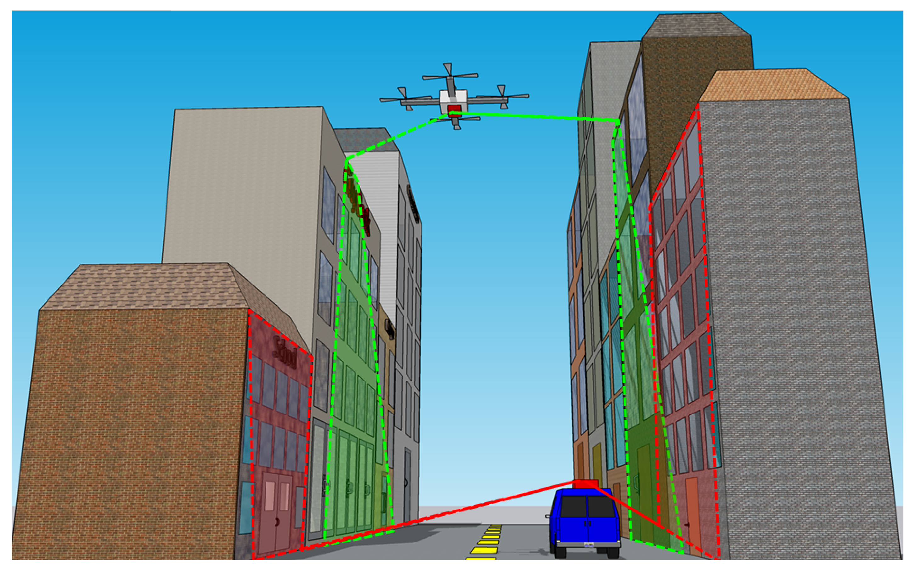
Such an accurate localization requires multiple aspects to be covered. The main concept is to benefit from the possible geometrical information that the surrounding environment offers. Such additional information could be, e.g., the parallel or perpendicular lines or planes of the environment. A scheme of the whole situation is illustrated in Figure 1 where different MSS are shown to be moving in an inner-city environment with high-rise buildings.

2.1. General Idea

The main idea is to establish a reliable connection between the sensor measurements and the surrounding environment that the MSS moves through. In the current paper, only the 3D scanner measurements are taken into consideration. Therefore, the first step is to know how the surrounding environment is defined and how this definition could be linked to the scanned data. In the LoD-2 3D city models, the buildings’ facades are defined by means of planes with defined parameters and vertices in a global coordinate system.

On the other hand, the ground is defined by a Digital Terrain Model (DTM), which contains a network of cells each having 2D coordinates plus the height information in a global coordinate system. One of the ways to link the measured data to the surrounding environment is to assign each scanned point either to a facade in the 3D city model or to a cell of the DTM. The scanned data are derived in the local coordinate system of the 3D scanner.

Therefore, if these data can be transformed to the same coordinate system in which the planes of the buildings and the heights of the ground are defined, the aforementioned connection could be established by assigning them to either the buildings or the ground. The taken georeferencing procedure in the current paper is in the “data-driven” category (explained in Section 1.1), which can be explained as follows:

Each scanned point is assigned to the closest DTM cell by calculating the 2D Euclidean distances. Afterward, the difference in the transformed height of the assigned scanned point—in the global coordinate system—and that of the DTM cell is derived. Next, the closest building’s facade to that point is derived, and then the point is assigned to either the DTM cell or the plane based on a certain defined threshold. A scheme of the assignment to the planes of the buildings is shown in Figure 2. In this figure, the green dots show the assigned scanned data to the building facades, which are shown by a grey plane.

The coordinate system of the far left of this figure is an indicator of the global coordinate system to which the scanned data should be transformed. Furthermore, the red dotted line of the far right side of this figure shows the distance threshold that is used through the assignment process. The idea is that the transformed scanned points with larger distances to the planes than the threshold are not considered through the whole filtering technique. The assignment methodology is taken from [48,49].

As can be seen, multiple points will be assigned to each plane of the 3D city model. Similarly, to each DTM cell, various scanned points are assigned, among which, the smallest point in height is selected as the ground representative at that specific location (Figure 3). The main issue is that the transformation could only be done by means of the MSS pose, which is unknown. Therefore, the main idea is to iteratively apply the transformation until the assignments are satisfactory. Such satisfaction lies in having appropriate transformation parameters, which, in turn, means having the correct MSS pose.

When it comes to real environments, such a “correctness” is challenging to be judged due to unknown “true” values; however, various criteria from different aspects could serve as means to decide upon the trustworthiness of the estimated pose values. In the current paper, the final results from the DSIEKF algorithm are compared with those derived from the IEKF algorithm that is also applied to the same environment.

2.2. Transformation to Global Coordinate System

To assign the scanned data to the planes of the buildings or the ground, they should be transformed to the global coordinate system by means of the transformation parameters. These parameters are, indeed, the 6-DoF of the MSS at each epoch in time. The transformation could be done as follows:

$${\mathbf{P}}_{glo}=\mathbf{t}+\mathbf{R}·{\mathbf{P}}_{loc}$$

(1)

where ${\mathbf{P}}_{glo}$ is the transformed laser scanner point cloud from the local to the global coordinate system. $\mathbf{t}$ and $\mathbf{R}$ are the translation parameters vector and rotation matrix, respectively. ${\mathbf{P}}_{loc}$ is the laser scanner point cloud in its local coordinate system. $\mathbf{R}$ is derived according to (2).

$$\mathbf{R}={\mathbf{R}}_{\omega }·{\mathbf{R}}_{\varphi }·{\mathbf{R}}_{\kappa }$$

(2)

where ${\mathbf{R}}_{\omega }$, ${\mathbf{R}}_{\varphi }$, and ${\mathbf{R}}_{\kappa }$ are rotations around the X, Y, and Z axes of the global coordinate system, respectively. These rotation matrices can be derived from (3).

$${\mathbf{R}}_{\omega }=\left[\begin{array}{ccc}1& 0& 0\\ 0& cos\omega & -sin\omega \\ 0& sin\omega & cos\omega \end{array}\right],{\mathbf{R}}_{\varphi }=\left[\begin{array}{ccc}cos\varphi & 0& sin\varphi \\ 0& 1& 0\\ -sin\varphi & 0& cos\varphi \end{array}\right],{\mathbf{R}}_{\kappa }=\left[\begin{array}{ccc}cos\kappa & -sin\kappa & 0\\ sin\kappa & cos\kappa & 0\\ 0& 0& 1\end{array}\right]$$

(3)

2.3. DSIEKF (Dual State Iterated Extended Kalman Filter)

An environment can have a great deal of geometrical information that would make the filtering approach inefficient if they were to be considered. This is especially true when it comes to IEKF where iterations are applied in the update step to overcome the linearization errors. Therefore, in DSIEKF, the main idea is to divide the state vector into two separate parts that should be estimated, interactively [6]. The reasoning behind such a division in the current paper is the fact that one vector can be fixed in size during all the epochs; whereas, the other vector can become larger over time due to the possible increasing information flow of the surrounding environment.

However, since such prior knowledge is taken from a reliable source—like the LoD-2 3D city models—the convergence of the second vector occurs faster than the first one. Consequently, the estimation time is decreased due to fixing the second vector after several iterations, and therefore only one vector needs to be estimated, which is considerably smaller in size than the case in which all the states are included in one vector (the IEKF methodology). A scheme of DSIEKF is presented in Figure 4, which shows the general idea of this algorithm and its application to the real scenario.

2.3.1. State Vector

As mentioned previously, there are two separate state vectors that should be estimated in the developed DSIEKF algorithm (see (4)). One that is related to the MSS and consists of the 6-DoF as well as the translational and angular velocities. The second state vector is related to the additional information of the environment, which, in the context of the current paper, consists of the plane parameters. The plane parameters are extracted from the LoD-2 3D city model and are taken as unknown parameters due to errors, such as generalization, which are irresistible while developing city models.

However, since the given information in such models are reliable enough, the convergence of these parameters occurs faster than the first state vector, which is a beneficial aspect of the DSIEKF algorithm, as also explained in Section 2.3. The two state vectors are:

$$\begin{array}{cc}\hfill {\mathbf{x}}_{state,k}^{\left(1\right)}& ={\left[\underset{\mathrm{translations}}{\underbrace{t_{x,k},t_{y,k},t_{z,k}}},\underset{\mathrm{orientations}}{\underbrace{{\omega }_k,{\varphi }_k,{\kappa }_k}},\stackrel{\text{translational velocities}}{\overbrace{V_{x,k},V_{y,k},V_{z,k}}},\stackrel{\text{angular velocities}}{\overbrace{{\mathrm{\Omega }}_{\omega ,k},{\mathrm{\Omega }}_{\varphi ,k},{\mathrm{\Omega }}_{\kappa ,k}}}\right]}^T\hfill \\ \hfill & ={\left[{\mathbf{T}}_k,{\mathbf{O}}_k,{\mathbf{V}}_k,{\mathrm{\Omega }}_k\right]}^T\hfill \\ \hfill {\mathbf{x}}_{plane,k}^{\left(2\right)}& =\left[\underset{\mathrm{plane}1}{\underbrace{{\mathbf{n}}_{1,k};d_{1,k}}};\underset{\mathrm{plane}2}{\underbrace{{\mathbf{n}}_{2,k};d_{2,k}}};\dots ;\underset{\mathrm{plane}\mathrm{E}}{\underbrace{{\mathbf{n}}_{E,k};d_{E,k}}}\right]\hfill \end{array}$$

(4)

where $\mathbf{T}$, $\mathbf{O}$, $\mathbf{V}$, and $\mathrm{\Omega }$ are translations, orientations, translational velocities, and angular velocities, respectively. $\mathbf{n}$ and d for each plane are representatives of its normal vector and distance to origin, respectively.

2.3.2. Observation Vector

Similar to the state vector that is separated into two parts, the observations are also divided into two categories each corresponding to one set of the unknown parameters. Correspondence in this case means to have observations that can be linked to the unknown parameters via mathematical formulations. The mathematical formulations, which are referred to as observation models, will then be used in the update step of the filter to modify the predicted states.

As given in (4), the first state vector consists of the MSS pose as well as its velocities. Two sets of observations could be linked to this state vector. One is the measured scanned points by means of the laser scanner and the second are the GNSS and IMU data. The scanned points are related to the first state vector through the transformation equation (see (1)), which should be used while assigning the points to the planes of the 3D city model as well as the DTM cells. These observations are measured in the local coordinate system of the scanner and can be written as follows:

$$\begin{array}{cc}\hfill {\mathbf{l}}_{scan,k}^{loc}& =\left[{\mathbf{l}}_{scan,1,k}^{loc};{\mathbf{l}}_{scan,2,k}^{loc};\dots ;{\mathbf{l}}_{scan,e,k}^{loc};\dots ;{\mathbf{l}}_{scan,E,k}^{loc}\right]\hfill \\ \hfill {\mathbf{l}}_{scan,e,k}^{loc}& =\left[{\mathbf{P}}_{e,1,k}^{loc};{\mathbf{P}}_{e,2,k}^{loc};\dots ;{\mathbf{P}}_{e,i,k}^{loc};\dots ;{\mathbf{P}}_{e,N_e,k}^{loc}\right]\hfill \\ \hfill {\mathbf{P}}_{e,i,k}^{loc}& ={\left[x_{e,i,k}^{loc},y_{e,i,k}^{loc},z_{e,i,k}^{loc}\right]}^T\hfill \end{array}$$

(5)

where ${\mathbf{l}}_{scan,k}^{loc}$ are all the scanned points assigned to the planes in epoch k, which could be divided into smaller groups each belonging to a specific plane. ${\mathbf{l}}_{scan,e,k}^{loc}$ shows the scanned points in epoch k that belong to the e-th plane. ${\mathbf{P}}_{e,i,k}^{loc}$ is the i-th 3D point—with x, y, and z coordinates in the local coordinate system of the scanner—that lies on the e-th plane and $N_e$ is the total number of assigned 3D points to plane e, which are measured in epoch k, respectively.

Similarly, the scanned points assigned to the DTM cells are as follows:

$$\begin{array}{cc}\hfill {\mathbf{l}}_{DTM,k}^{loc}& =\left[{\mathbf{l}}_{DTM,1,k}^{loc};{\mathbf{l}}_{DTM,2,k}^{loc};\dots ;{\mathbf{l}}_{DTM,c,k}^{loc};\dots ;{\mathbf{l}}_{DTM,C,k}^{loc}\right]\hfill \\ \hfill {\mathbf{l}}_{DTM,c,k}^{loc}& ={\mathbf{P}}_{c,k}^{loc}={\left[x_{c,k}^{loc},y_{c,k}^{loc},z_{c,k}^{loc}\right]}^T\hfill \end{array}$$

(6)

where ${\mathbf{l}}_{DTM,k}^{loc}$ are all the scanned points assigned to the DTM cells in epoch k, which could be divided into smaller groups each belonging to a specific cell. Each group contains one 3D point ${\mathbf{l}}_{DTM,c,k}^{loc}$, which shows the scanned point in epoch k—with x, y, and z coordinates in the local coordinate system of the scanner—that belongs to the c-th cell. C shows the total number of DTM cells in epoch k to which a scanned point is assigned.

On the other hand, if the GNSS and IMU data are available in each epoch, they can also be related to the first state vector. As the first state vector contains the 6-DoF, which are directly the GNSS and IMU measurements. Consequently, the first observation vector corresponding to the first state vector is as follows:

$$\begin{array}{cc}\hfill {\mathbf{l}}_k^{\left(1\right)}& =\left[{\mathbf{l}}_{scan,k}^{loc};{\mathbf{l}}_{DTM,k}^{loc};{\mathbf{l}}_{pose,k}^{glo}\right]\hfill \\ \hfill {\mathbf{l}}_{pose,k}^{glo}& ={\left[\underset{\mathrm{GNSS}\mathrm{data}}{\underbrace{t_{x,k}^{GNSS},t_{y,k}^{GNSS},t_{z,k}^{GNSS}}},\underset{\mathrm{IMU}\mathrm{data}}{\underbrace{{\omega }_k^{IMU},{\varphi }_k^{IMU},{\kappa }_k^{IMU}}}\right]}^T\hfill \end{array}$$

(7)

However, as previously mentioned, due to technical issues, GNSS and IMU data (${\mathbf{l}}_{pose,k}^{glo}$) were not reliable enough for the prototype UAV, and hence they are not considered in the current paper.

With a similar justification as for the first state vector, the corresponding observations of the second state vector should also be selected. In the current paper, these measurements are not only the scanned data of the laser scanner but also the corner points of the 3D city model. These two sets of measurements could be related to the second state vector via the plane equation.

Otherwise stated, both the transformed scanned data of the laser scanner as well as the corner points of the facades in the 3D city model should satisfy the mathematical equation of their corresponding plane if, and only if, the plane parameters are estimated correctly. Equation (8) shows the corner points measurements with a similar definition as given for Equation (5). The only difference is that the corner points are already in the global coordinate system, and hence the transformation is not applied to them.

$$\begin{array}{cc}\hfill {\mathbf{l}}_{corner,k}^{glo}& =\left[{\mathbf{l}}_{corner,1,k}^{glo};{\mathbf{l}}_{corner,2,k}^{glo};\dots ;{\mathbf{l}}_{corner,e,k}^{glo};\dots ;{\mathbf{l}}_{corner,E,k}^{glo}\right]\hfill \\ \hfill & =\left[{\mathbf{P}}_{e,1,k}^{glo};{\mathbf{P}}_{e,2,k}^{glo};\dots ;{\mathbf{P}}_{e,i,k}^{glo};\dots ;{\mathbf{P}}_{e,N_c,k}^{glo}\right]\hfill \\ \hfill {\mathbf{P}}_{e,i,k}^{glo}& ={\left[X_{e,i,k}^{glo},Y_{e,i,k}^{glo},Z_{e,i,k}^{glo}\right]}^T\hfill \end{array}$$

(8)

Consequently, the second observation vector related to the second state vector can be written as follows:

$${\mathbf{l}}_k^{\left(2\right)}=\left[{\mathbf{l}}_{scan,k}^{loc};{\mathbf{l}}_{corner,k}^{glo}\right]$$

(9)

2.3.3. System Equations

System equations are used in the prediction step of the DSIEKF to model the dynamic behavior of the MSS. Using such equations, it is possible to derive the state of the MSS in the current epoch based on its states in the previous epoch. In [50], a detailed dynamic model for UAVs is given that takes into account significant effects and disturbances. In the current paper, however, a simple linear model is used. The reason for this is the high number of observations as well as the integration of the additional information in the update step, which we think could compensate the simply used dynamic model. In the proposed methodology of DSIEKF, two system equations are used each for one of the state vectors, which can be written as (10):

$$\begin{array}{cc}\hfill {\mathbf{x}}_k^{\left(1\right)}& ={\mathbf{f}}^{\left(1\right)}({\mathbf{x}}_{k-1}^{\left(1\right)},{\mathbf{u}}_{k-1}^{\left(1\right)},{\omega }_{k-1}^{\left(1\right)})\hfill \\ \hfill {\mathbf{x}}_k^{\left(2\right)}& ={\mathbf{f}}^{\left(2\right)}({\tilde{\mathbf{x}}}_k^{\left(2\right)},{\mathbf{u}}_k^{\left(2\right)},{\omega }_k^{\left(2\right)})\hfill \end{array}$$

(10)

where ${\mathbf{x}}_k^{\left(1\right)}$, ${\mathbf{f}}^{\left(1\right)}$, ${\mathbf{x}}_{k-1}^{\left(1\right)}$, ${\mathbf{u}}_{k-1}^{\left(1\right)}$, and ${\omega }_{k-1}^{\left(1\right)}$ all belong to the first state vector and indicate the states in epoch k, the corresponding (nonlinear) system equation, the states in epoch $k-1$, the control unit, and the system noise. A similar definition applies to the elements of the second Equation in (10), except that, for the second state vector, the already available information in the current epoch (${\tilde{\mathbf{x}}}_k^{\left(2\right)}$) are to be modified. In the current paper, linear system equations are claimed to be sufficient within the prediction step. Therefore, such equations for both of the state vectors can be written as follows:

$$\begin{array}{cc}\hfill {\mathbf{x}}_k^{\left(1\right)}& ={\mathbf{F}}_x^{\left(1\right)}·{\mathbf{x}}_{k-1}^{\left(1\right)}+{\omega }_{k-1}^{\left(1\right)}\hfill \\ \hfill {\mathbf{x}}_k^{\left(2\right)}& ={\mathbf{F}}_x^{\left(2\right)}·{\tilde{\mathbf{x}}}_k^{\left(2\right)}+{\omega }_k^{\left(2\right)}\hfill \\ \hfill {\mathbf{F}}_x^{\left(1\right)}& =\left[\begin{array}{cc}{\mathbf{I}}_{[6\times 6]}& diag\left(\right[\mathrm{\Delta }\tau ,\mathrm{\Delta }\tau ,\mathrm{\Delta }\tau ,\mathrm{\Delta }\tau ,\mathrm{\Delta }\tau ,\mathrm{\Delta }\tau \left]\right)\\ {\mathbf{0}}_{[6\times 6]}& {\mathbf{I}}_{[6\times 6]}\end{array}\right]\hfill \\ \hfill {\mathbf{F}}_x^{\left(2\right)}& ={\mathbf{I}}_{[4·E_k\times 4·E_k]}\hfill \end{array}$$

(11)

where ${\mathbf{F}}_x^{\left(1\right)}$ and ${\mathbf{F}}_x^{\left(2\right)}$ are the “transition matrices”, $\mathbf{I}$ is an identity matrix, $\mathrm{\Delta }\tau$ is the time period between two consecutive epochs, and $E_k$ is the total number of planes that are detected in epoch k.

The Variance Covariance Matrix (VCM) of the system noise consists of two parts: a part related to the MSS states and a part related to the planes of the 3D city model. To build the predicted VCM of the MSS states, the concept of “Continuous White Noise Acceleration Model” of [51] is used within the current paper. In this model, the main idea is the contribution of the MSS acceleration to the VCM of the system noise. The authors in [51] claimed that, in systems with constant velocity, the expected acceleration over all the epochs is zero; however, the velocity undergoes slight changes, and therefore the VCM of the system noise is affected by the resulting random acceleration. Inspired by such a claim, the VCM of the system noise within the context of this paper is formulated as follows:

$$\begin{array}{cc}\hfill {\mathrm{\Sigma }}_{\omega \omega }^{\left(1\right)}& ={\mathrm{\Sigma }}_{\omega \omega ,stat{e}^{\left(1\right)}}=\mathbf{Q}·\tilde{\mathbf{q}}\hfill \\ \hfill \mathbf{Q}& =\left[\begin{array}{cc}\frac{{(\mathrm{\Delta }\tau )}^3}{3}·{\mathbf{I}}_{6\times 6}& {\mathbf{0}}_{6\times 6}\\ {\mathbf{0}}_{6\times 6}& (\mathrm{\Delta }\tau )·{\mathbf{I}}_{6\times 6}\end{array}\right]\hfill \\ \hfill \tilde{\mathbf{q}}& =diag({\mathbf{q}}_T,{\mathbf{q}}_O,{\mathbf{q}}_V,{\mathbf{q}}_{\mathrm{\Omega }})\hfill \\ \hfill {\mathbf{q}}_T& =[a,a,a],{\mathbf{q}}_O=[b,b,b],{\mathbf{q}}_V=[c,c,c],{\mathbf{q}}_{\mathrm{\Omega }}=[d,d,d]\hfill \end{array}$$

(12)

where ${\mathrm{\Sigma }}_{\omega \omega }^{\left(1\right)}$ is the VCM of the system noise corresponding to the first state vector, $\mathbf{Q}$ is derived based on the particular solution of the superposition law that is applied to the system noise (more detail provided in [51]), and $\tilde{\mathbf{q}}$ are the continuous-time process noise intensities that appear as parameters to be designed, which are assumed to be constant over time for all the states parameters. Numerical values considered for the application within the current paper are given in

Table 1. Applied accuracy and design parameters ($\tilde{\mathbf{q}}$) of the system noise values.

Initial State Accuracy	${\sigma }_{T,0}=$$0.5$ m
	${\sigma }_{O,0}=$$0.2^{\circ }$
	${\sigma }_{V,0}=$ 1 m/s
	${\sigma }_{\mathrm{\Omega },0}=$$1^{\circ }$/s
	${\sigma }_{n,0}=$ 0.001
	${\sigma }_{d,0}=$ 0.03 m
	${\sigma }_{CP,0}=$ 0.03 m
System Noise	$\mathrm{\Delta }\tau =$ approx. 0.1 s between each two epochs
	$a=$ 270 m${}^2$/s${}^3$
	$b=$ 0.08 rad${}^2$/s${}^3$
	$c=$ 0.02 m${}^2$/s${}^3$
	$d=$ 7.62 × 10${}^{-4}$ rad${}^2$/s${}^3$
	${\sigma }_{n,\omega }=$ 0
	${\sigma }_{d,\omega }=$ 0
Measurement Noise	${\sigma }_{LS}=$ 0.02 m
	${\sigma }_{CP}=$ 0.03 m
	${\sigma }_{DTM}=$ 0.2 m

.

2.3.4. Measurement Equations

As already mentioned in Section 2.3.2, observation models link the measurements to the unknown parameters. These models are then used in the update step of the filter to modify the predictions of the states. As also explained in Section 1.2, observation models are of two types referred to as GMM and GHM. They can be formulated as follows (the first equation corresponding to GMM and the second equation corresponding to GHM):

$$\begin{array}{cc}\hfill {\mathbf{l}}_k+{\nu }_k& ={\mathbf{H}}_{x,k}{\mathbf{x}}_k\hfill \\ \hfill \mathbf{h}({\mathbf{l}}_k+{\nu }_k,{\mathbf{x}}_k)& =\mathbf{0}\hfill \end{array}$$

(13)

where $\mathbf{l}$, $\mathbf{x}$, ${\mathbf{H}}_x$, $\nu$, $\mathbf{h}$ are the measurements vector, state vector, design matrix, measurements noise with VCM ${\mathrm{\Sigma }}_{\nu \nu }$, and the nonlinear observation model in epoch k, respectively.

For the first state vector, if GNSS and IMU data are available, an observation model of GMM type could be used, which can be written as follows:

$$\begin{array}{cc}\hfill {\mathbf{l}}_{pose,k}^{glo}+{\nu }_k& ={\mathbf{x}}_{state,pose,k}^{\left(1\right)}\hfill \\ \hfill {\mathbf{x}}_{state,pose,k}^{\left(1\right)}& ={\left[\underset{\mathrm{translations}}{\underbrace{t_{x,k},t_{y,k},t_{z,k}}},\underset{\mathrm{orientations}}{\underbrace{{\omega }_k,{\varphi }_k,{\kappa }_k}}\right]}^T\hfill \end{array}$$

(14)

where ${\mathbf{l}}_{pose,k}^{glo}$, ${\nu }_k$, and ${\mathbf{x}}_{state,pose,k}^{\left(1\right)}$ are the GNSS and IMU data as measurements, observations noise, and the unknown 6-DoF, respectively. These 6-DoF which are part of the first state vector are the pose parameters.

However, in the current paper, due to unavailable GNSS and IMU data, such GMM observation models are not considered. Nonetheless, the prototype UAV is also equipped with a 3D laser scanner, which constantly captures the surrounding environment. Furthermore, corner points of the buildings within the 3D city model are considered as additional observations to ensure higher redundancy and, hence, more accurate estimations.

On the other hand, as explained in Section 2.3.1, one of the state vectors to be estimated contains geometrical parameters of the surrounding environment. In order to derive this state vector, a suitable relationship should be established that links it to the 3D scanned data from the laser scanner and corner points of the 3D city model. Such a relationship could be the Hesse form of a plane, which has a general type as the second Equation in (13) and, hence, is a GHM:

$${\mathbf{n}}_{\mathbf{x}}k·{\mathbf{X}}_k^{glo}+{\mathbf{n}}_{\mathbf{y}}k·{\mathbf{Y}}_k^{glo}+{\mathbf{n}}_{\mathbf{z}}k·{\mathbf{Z}}_k^{glo}-{\mathbf{d}}_k=\mathbf{0}$$

(15)

where ${\mathbf{n}}_{\mathbf{x}}$, ${\mathbf{n}}_{\mathbf{y}}$, and ${\mathbf{n}}_{\mathbf{z}}$ are the planes’ normal vector parameters. $\mathbf{d}$ is the planes’ distance parameter vector. ${\mathbf{X}}_k^{glo}$, ${\mathbf{Y}}_k^{glo}$, and ${\mathbf{Z}}_k^{glo}$ are the global point coordinates. In case of the scanned points by means of a 3D laser scanner, a transformation should be applied, which is to bring the points from the local coordinate system to the global one. Such a transformation is done according to (1). In case of corner points, no transformation is required, since these points are already in the same coordinate system in which the plane parameters are defined.

As explained in Section 2.1, the ground is defined by relating the scanned points to the DTM of the environment. Such a relation is derived based on the following equation of GHM type, which compares the transformed height of the scanned point in the global coordinate system to that of the DTM cell:

$${\mathbf{Z}}^{glo,DTM}-{\mathbf{Z}}_{DTM}=0$$

(16)

where ${\mathbf{Z}}^{glo,DTM}$ and ${\mathbf{Z}}_{DTM}$ are the transformed height of the scanned points to the global coordinate system and height information of the DTM, respectively. Unlike the plane parameters that are taken as unknown parameters through the filter, the height information is taken as deterministic values, and therefore they are not modified.

2.3.5. Nonlinear Equality Constraints

Aside from the additional geometrical information of the environment, sometimes it is also possible to engage certain restrictions that lead to more accurate estimations. Such restrictions, which are also taken from the surroundings, appear as mathematical formulations that could be integrated into the filter. In the current paper, the unity of the planes’ normal vectors are taken as the geometrical constraints that have to be fulfilled by the final estimated plane parameters.

There are a number of methods for applying geometrical constraints on the filtered states [38]. In the current paper, the projection approach is used, mainly since it is the chosen strategy in [1,30,31] as well. The considered geometrical constraint could be formulated as follows:

$$\sqrt{n_x^2+n_y^2+n_z^2}=1$$

(17)

where $n_x$, $n_y$, and $n_z$ are the normal vector parameters of each plane. This geometrical constraint is of nonlinear type and, therefore, a Taylor series expansion is used for linearization within the projection method in [1,6]. The linearized form of a nonlinear constraint (as (18)) by means of the first degree Taylor polynomial is as given in (19).

$$g\left(x_k\right)=b$$

(18)

where g is a nonlinear mathematical function that has an exact value of b in a true state $x_k$.

$$g\left(x_k\right)=g\left({\widehat{x}}_k^{-}\right)+g^{\prime }\left({\widehat{x}}_k^{-}\right)(x_k-{\widehat{x}}_k^{-})$$

(19)

where ${\widehat{x}}_k^{-}$ and $g^{\prime }$ are the predicted values of $x_k$ and the derivative of g with respect to ${\widehat{x}}_k^{-}$, respectively.

2.3.6. Initialization

Initializing KF realizations is always a challenging task, as inappropriate initial values lead to filter divergence and, hence, unreliable outputs. Therefore, it is preferable to choose such values, reasonably and based on proper judgments of the overall scenario. For the current paper, the initial translation and orientation parameters are taken from the GNSS and IMU data at the beginning of the experiment. The initial velocities are taken as zero values, and the initial plane parameters are extracted directly from the LoD-2 3D city model. Similar to the parameters of the state, their VCM should also be reasonably initiated.

In (20)–(27), the order and arrangement of the initial state parameters as well as their VCM is given. Numerical values considered for the application within the current paper are given in Table 1.

$${\mathbf{x}}_{state,0}^{\left(1\right)}={\left[{\mathbf{T}}_0^{GNSS},{\mathbf{O}}_0^{IMU},{\mathbf{V}}_0,{\mathrm{\Omega }}_0\right]}^T$$

(20)

$${\mathbf{T}}_0^{GNSS}={\left[t_{x,0}^{GNSS},t_{y,0}^{GNSS},t_{z,0}^{GNSS}\right]}^T,{\mathbf{O}}_0^{IMU}={\left[{\omega }_0^{IMU},{\varphi }_0^{IMU},{\kappa }_0^{IMU}\right]}^T$$

(21)

$${\mathbf{V}}_0={\left[0,0,0\right]}^T,{\mathrm{\Omega }}_0={\left[0,0,0\right]}^T$$

(22)

$${\mathbf{x}}_{plane,0}^{\left(2\right)}=\left[{\mathbf{n}}_{1,0};d_{1,0};{\mathbf{n}}_{2,0};d_{2,0};\dots ;{\mathbf{n}}_{E,0};d_{E,0}\right]$$

(23)

$${{\Sigma }}_{xx,0}^{\left(1\right)}=diag({\sigma }_{T,0}^2,{\sigma }_{O,0}^2,{\sigma }_{V,0}^2,{\sigma }_{\mathrm{\Omega },0}^2)$$

(24)

$${\sigma }_{T,0}^2=diag({\sigma }_{T,0}^2,{\sigma }_{T,0}^2,{\sigma }_{T,0}^2),{\sigma }_{O,0}^2=diag({\sigma }_{O,0}^2,{\sigma }_{O,0}^2,{\sigma }_{O,0}^2)$$

(25)

$${\sigma }_{V,0}^2=diag({\sigma }_{V,0}^2,{\sigma }_{V,0}^2,{\sigma }_{V,0}^2),{\sigma }_{\mathrm{\Omega },0}^2=diag({\sigma }_{\mathrm{\Omega },0}^2,{\sigma }_{\mathrm{\Omega },0}^2,{\sigma }_{\mathrm{\Omega },0}^2)$$

(26)

$${{\Sigma }}_{xx,0}^{\left(2\right)}=diag({\sigma }_{n,0}^2,{\sigma }_{d,0}^2,{\sigma }_{n,0}^2,{\sigma }_{d,0}^2,\dots ,{\sigma }_{n,0}^2,{\sigma }_{d,0}^2)$$

(27)

2.4. Workflow

The workflow of the developed DSIEKF that is applied to the real scenario is given in Algorithm 1. For better comprehension of the overall procedure, a sketch of the algorithm is also provided in Figure 5. The given algorithm is based on the one given by [6] but modified and made consistent with the real environment. The modification lies mainly in the VCM of the system noise and the integration of the DTM model into the filter as explained in Section 2.1 and Section 2.3.3, respectively.

Furthermore, the information-based georeferencing methodology—referred to as IEKF in the current paper—that was developed by [30] and applied by [1] on a simulated UAV environment is also considered. The main reason for doing so is to compare the two methodologies. When it comes to real environments, no true values exist, and therefore comparing the outputs of two algorithms on a common scenario could be one way to examine the final results. In lines 1 to 4 of Algorithm 1, the corresponding system and observation models of the two state vectors are defined.

Algorithm 1: Dual State Iterated Extended Kalman Filter (DSIEKF) with nonlinear equality constraints.

In line 5, the first state vector and its corresponding VCM are initialized. In line 6, a matrix is initialized, which will be filled in as given in line 41. The main aim is to store the modified planes in this matrix so that they are not modified anymore if they are captured in the next epochs (as also indicated in line 10). In each epoch, the scanned data are assigned to the surrounding building models, and thus the planes information could directly be extracted from the 3D city model.

This extracted information along with the considered accuracy values are taken as the initialized values of the second state vector and its corresponding VCM (as given in line 9). Lines 12 to 15 of the algorithm deal with predicting both of the state vectors and their corresponding VCM. For predicting the VCM of the second state vector (line 15), a user-defined factor $\lambda$ is used, which is referred to as the “forgetting factor” and ranges from 0 to 1 [33]. The main idea of using such a factor is to have an exponentially decaying weighting on the past data [33].

For the current paper, this factor was chosen to be 0.5. Lines 17 to 40 show the update steps in which both of the predicted state vectors are modified by taking into their corresponding observations. The first update step (lines 19 to 24) deals with modifying the first state vector and its corresponding observations within an outer loop indicated by m. Afterward, the second state vector and its corresponding observations should be modified, which is indicated in line 27 and happens within an inner loop indicated by n.

Therefore, similar computations as of lines 19 to 24 should be repeated but this time for the second state vector. In this update step, anywhere that the first state vector and its corresponding observations are needed, the modified ones from lines 22 and 24 should be used. Similarly, for updating the first state vector, anywhere that the second state vector and its corresponding observations appear, the most recent modified ones should be used.

Since the geometrical constraints should be applied on the second state vector, they are applied in the inner loop while updating the second state vector (lines 31 to 33). The inner loop is only entered if $max(\mathrm{\Delta }\mathbf{x})$ exceeds a certain threshold indicated by $c_{stop}$. $\mathrm{\Delta }\mathbf{x}$ is the difference between the updated second state vector in two consecutive iterations. $c_{stop}$ is chosen to be ${10}^{-4}$ in the current paper.

3. Application

In geodesy, capturing the surrounding environment for further analytical purposes is a common task that is sought in different ways based on the demand. In certain cases, static measurements are sufficient to partly survey the environment; whereas, in other cases, kinematic measurements are preferred in order to capture different parts of it. Various possibilities exist when it comes to kinematic measurements among which using trolleys or vehicles equipped with multiple sensors could be mentioned. However, sometimes the environment is complicated enough to not allow using the aforementioned kinematic means.

In those cases, the UAVs are proper choices for mapping purposes, which can usually be steered in desired heights and along favorable paths. They usually have a compact and light-weight design, which enables their flexible movements. As mentioned previously, to investigate different aspects of UAV-based problems, the GIH and IPI at LUH developed a prototype Unmanned Aerial System (UAS) where a UAV is equipped with GNSS, IMU, a 3D laser scanner, and camera units within the course of a joint project. In Figure 6, a scheme of such a UAV is presented followed by further details in the succeeding sections.

3.1. Overview of the Real Environment

The mentioned prototype UAV is equipped with GNSS, IMU, a 3D laser scanner, and camera units mounted on a gimbal for better stabilization and damping. The 3D laser scanner is a Velodyne Puck (VLP-16) with 16 individual scan lines, a $30\times 360$ field of view, and a 3 cm range accuracy [52]. The rotation frequency was selected to be 10 Hz, which corresponds to 30,000 3D points per 360 rotation. In order to have a reliable synchronization and data combination with the other mounted sensors, the GNSS time stamps are applied to the scanned data via additional GNSS units. Moreover, although GNSS and IMU data are available through the whole measurement process, they are neglected in this paper. Camera units are used in the joint project; however, they are neglected here, since integrating camera images in the filter is out of the scope of the current paper. An overview of the whole system can be seen in Figure 7.

Within the project, an inner courtyard was selected as the environment in which the UAV carried out the measurements at a height of almost 2 m. A map-based representation of the area along with its corresponding images is shown in Figure 8. Such a selected spacious environment has perfect conditions for evaluating the performance of both the DSIEKF and IEKF algorithms.

3.2. Additional Complementary Information

As previously indicated, the IEKF and DSIEKF algorithms are based on available and reliable information that could be extracted from the environment in which the MSS moves through. In the current paper, such information is selected to be the LoD-2 3D city model of Hanover along with the DTM due to their availability for the environment of interest. These complementary information are extracted from [54,55].

In Figure 9, an overview of such additional information for the current project is presented. The DTM in the current paper refers to the German height reference network (Deutsches Haupthöhennetz—DHHN2016) which has a grid width of 1 m with the accuracy of height information less than 0.3 m [55]. Due to the generalization process, the LoD-2 3D city model has deviations up to the centimeter or even decimeter level compared to the real environment, which is the main reason for taking such additional information as unknown parameters to be estimated in the filtering process.

3.3. Analysis Material and Requisites

The considered values for the initial state accuracy, system, and measurement noise are selected as given in Table 1. In this table, the subscripts “LS” and “CP” refer to the laser scanner and corner points data and the definition of the other subscripts is consistent with those given in the mathematical formulations of this paper. The considered initial state accuracy of translations (${\sigma }_{T,0}$), orientations (${\sigma }_{O,0}$), and translational and angular velocities (${\sigma }_{V,0}$ and ${\sigma }_{\mathrm{\Omega },0}$) are selected based on the installed sensors on the UAV platform.

For example, the selected value of ${\sigma }_{T,0}=0.5$ m is based on the accuracy of the used GNSS unit. Since no uncertainty information of either the plane parameters or the corner points is given in the LoD-2 3D city model, they were selected based on the accuracy of this digitized model, which is usually at the centimeter or even decimeter level. Therefore, the values of ${\sigma }_{n,0}$, ${\sigma }_{d,0}$, and ${\sigma }_{CP,0}$ are user-defined. As previously mentioned in Section 2.3.3, the accuracy of system noise is based on several parameters that should be designed.

Such a design should be based on the system dynamics as well as the affecting elements of its surrounding environment, such as wind. However, modeling these influencing factors is complicated and not in the scope of the current paper. Therefore, to select the values of a, b, c, and d, a sensitivity analysis was performed in order to see the effect of different values on the overall estimations and, hence, select those values that lead to more optimized solutions.

Furthermore, in the current paper, the accuracy of the measurement noise for the corner points and DTM heights was also selected based on the accuracy of the LoD-2 and DTM models. Additionally, the initial state vectors were selected accurately enough for the algorithms to not encounter divergence problems. Such a realization is based on a comparison between the first initial values of the GNSS and IMU data and the geographic coordinates of the captured measurement area.

Furthermore, processing all the measurements is, on one hand, computationally inefficient and, on the other hand, unnecessary due to the similar information content of nearby observations. Therefore, down-sampling is an irresistible step that is usually taken into account while analyzing real scenarios. In the current paper, it is applied by defining spatial boxes with a grid size of 1 m around the laser scanner measurements and averaging the neighbored observations.

For that, the already built-in MATLAB library (pcdownsample) was used. Performing this step led to a considerable decrease in the number of scanned data. As an example, in the first epoch, the scanned measurements were reduced in size from around 22,000 points to about 1700 points. However, by applying this down-sampling library, the original observations were changed to artificial ones due to averaging. Nonetheless, since the average is based on the real measurements, it is claimed that they can be treated as original observations to test the performance of the algorithms on a real environment.

In the following, the final results alongside the related discussions are presented. The algorithms are implemented in MATLAB R2019b programming language which are then performed on a windows-based computer with Intel(R) Xeon(R) CPU E5-1650 v2 @ 3.50 GHz 3.50 GHz processor and 64 GB RAM.

4. Results

In the following, the results of the DSIEKF along with those derived from the IEKF algorithm are depicted. As previously mentioned, the main difference between these two methodologies is the way the unknown parameters are treated and estimated within the whole filtering process. Therefore, having both of the algorithms applied to the same real scenario provides a good opportunity to not only compare their performance but also to validate the results of each methodology with respect to the other.

In general, “validation” can be done when the true values of the unknowns are available; however, in real environments, such values are never known. In principle, deriving the reference solutions in practical applications is feasible, but it requires great effort, which might not be always efficient. The authors in [32] derived a linear reference trajectory for a practical application by means of a laser tracker.

However, due to limited range measurements of a laser tracker, such a reference solution is only carried out for a small part of the trajectory. Therefore, other strategies should be taken to evaluate the final results. In the current paper, the procedure for doing so is to compare the estimations of both the algorithms with each other.

In Figure 10, the derived trajectories by means of the two algorithms are given from the top view. the derived trajectories have no considerable divergence from the real covered path by the UAV for they have all remained in the same environment where the UAV moved along.

In Figure 11 and Figure 12, the absolute differences between the estimated translation and orientation parameters over all the epochs are shown, respectively. In these figures, $\mathrm{\Delta }{\mathbf{t}}_x$, $\mathrm{\Delta }{\mathbf{t}}_y$, and $\mathrm{\Delta }{\mathbf{t}}_z$ correspond to the absolute differences between the estimated translation parameters along X, Y, and Z axes. Similarly, $\mathrm{\Delta }\omega$, $\mathrm{\Delta }\varphi$, and $\mathrm{\Delta }\kappa$ represent the absolute differences between the estimated orientations along the three main axes.

According to Figure 11, the difference between the estimations of ${\mathbf{t}}_x$ and ${\mathbf{t}}_y$ are not as large as ${\mathbf{t}}_z$. The reason for that is having multiple building facades in the surroundings that provide additional information for the filters. These building models are also modified within the filters, and therefore any errors from sources, such as generalization, are well compensated for through the estimation process. Consequently, both of the filters deliver similar ${\mathbf{t}}_x$ and ${\mathbf{t}}_y$ estimations.

In Figure 12, the $\kappa$ estimations from the two filters are similar. The reason is due to the small movements of the UAV around the Z axis and the suitable initialization in both filters. In

Table 2. The maximum difference between the estimated pose parameters over 1902 epochs by means of IEKF and DSIEKF.

${{\Delta }}_{{\mathit{t}}_{\mathit{x}}}$ [m]	${{\Delta }}_{{\mathit{t}}_{\mathit{y}}}$ [m]	${{\Delta }}_{{\mathit{t}}_{\mathit{z}}}$ [m]	${{\Delta }}_{\mathit{\omega }}[\circ ]$	${{\Delta }}_{\mathit{\varphi }}[\circ ]$	${{\Delta }}_{\mathit{\kappa }}[\circ ]$
0.4	0.6	2	0.06	0.08	0.02

, the maximum of these values over 1902 epochs is given. the two algorithms greatly disagree with each other in ${\mathbf{t}}_z$ estimations. The reason is claimed to be the DTM height information that is taken as deterministic values in both of the algorithms.

As explained in Section 3.2, the accuracy of height information is less than 0.3 m. Unlike the plane parameters that are taken as unknowns to be modified by the filters, this height information is considered constant, which subsequently leads to less qualitative results compared to the other transformation parameters. Such a claim is also approved by taking the mean standard deviation of the estimated parameters (in 1902 epochs) that are shown in

Table 3. Measures of different variables over 1902 epochs for each algorithm. T: Duration of the update step, $\sigma$: Mean standard deviation of the state parameters.

Algorithm	T [min]	${\mathit{\sigma }}_{{\mathit{t}}_{\mathit{x}}}$ [mm]	${\mathit{\sigma }}_{{\mathit{t}}_{\mathit{y}}}$ [mm]	${\mathit{\sigma }}_{{\mathit{t}}_{\mathit{z}}}$ [mm]	${\mathit{\sigma }}_{\mathit{\omega }}[\circ ]$	${\mathit{\sigma }}_{\mathit{\varphi }}[\circ ]$	${\mathit{\sigma }}_{\mathit{\kappa }}[\circ ]$
IEKF	28	6	6.2	9.4	0.03	0.03	0.004
DSIEKF	15	1.5	1.6	8.8	0.02	0.02	0.003

.

The standard deviation of the estimated translation parameter along the Z axis was larger than the other ones in both of the algorithms. Moreover, by comparing the standard deviation of the other estimated pose parameters, it is seen that, in general, not only did the DSIEKF take a shorter time to run but it also delivered better estimations.

Figure 13 and Figure 14 show the maximum absolute differences between the estimated planes’ normal vectors and distances to the origin and their given values in the 3D city model, respectively. In Figure 13 and for each epoch, the maximum value was derived for the absolute differences between the three components of all the normal vectors. Similarly, in Figure 14 and for each epoch, the maximum value was derived for the absolute differences between the distance parameters.

DSIEKF delivers estimations that are closer to the available values in the 3D city model than those derived by IEKF. Having such results approves the aforementioned justification of the error propagation effect even more. However, as mentioned in Section 3.2, the LoD-2 3D city model itself is prone to errors due to generalization, and therefore having closer estimated plane parameters to such a model should not be interpreted as superiority of DSIEKF over IEKF in sense of accuracy.

Nonetheless, no error-free true information of the surrounding environment exists, and, in the context of these two filters, the LoD-2 3D city model is taken as a reliable source. Therefore, based on such a consideration, it could be claimed that DSIEKF delivers more reliable estimations than IEKF, although the difference between the two filters is not significant.

Finally, the duration of the update time for both of the algorithms is shown in Figure 15. The reason for only showing the update time instead of the overall time is to show how the main difference between the two algorithms—which is the update step—influences the computation time. In Table 3, it is given that, for 1902 epochs, IEKF takes 28 min to finish the update steps, while DSIEKF takes only 15 min. Therefore, the DSIEKF algorithm is about 45% faster than the IEKF.

The reason for having faster computations in DSIEKF is, first, the significantly smaller matrices in size to be inverted than in the IEKF algorithm. Such matrices can be found, e.g., in line 20 of Algorithm 1, which, due to their size, are inverted faster in the following lines of the same algorithm than in IEKF. Secondly, after several iterations, lines 25 to 34 of Algorithm 1 are neglected, which leads to a considerable decrease in the overall estimation time of the update step.

5. Discussion

As shown in Section 4, outcomes of the DSIEKF for georeferencing a real case UAV are compared to those of the IEKF. The main reasons for doing so are, first, the similar principle that forms the basis of these two algorithms. Secondly, as also stated before, no ground truth solutions are available for this case study in order to validate the DSIEKF performance. The final estimated states along the trajectory by the two algorithms are shown to have a maximum difference of 60 cm, with an average standard deviation of around 2 and 6 mm by DSIEKF and IEKF, respectively.

The height estimations are shown to have a maximum difference of around 2 m by the two methodologies with an average standard deviation of around 9 mm for both the algorithms. Having such a significant difference between the height estimations is claimed to be due to the inaccurate height information that are taken as deterministic values into account. The orientation estimations from the two algorithms are shown to be in the same range. A maximum difference of around 0.1 degree was the largest difference between the estimations of the two algorithms, which was derived for the orientation around the Y axis.

In general, the DSIEKF estimations were derived with smaller standard deviations, which could be an indicator for the better performance of this methodology compared to the IEKF. It is claimed that such results are due to the state division strategy that is taken in DSIEKF, which avoids propagating the measurements uncertainties in the iterations of the update step, repeatedly. in other words, in the IEKF algorithm, where all unknown parameters in a vector are considered, the number of iterations required to reach an optimized solution is unnecessarily increased to fulfill a specified threshold that should be fulfilled by all estimated parameters.

Having all the unknown parameters in one vector to be estimated would mean to have more measurements that are iteratively used, which, consequently, produces a higher error propagation effect. Conversely, in DSIEKF, the second state vector is estimated in a lower number of iterations, which, in tur,n means considering fewer observations for deriving the pose parameters and, thus, less propagated uncertainties. The update time needed to carry out the estimations for the whole scenario by DSIEKF is nearly half of time taken by the IEKF algorithm, which is another important aspect of the DSIEKF methodology.

6. Conclusions and Outlook

The focus of this paper is to show the functionality of the IEKF and DSIEKF algorithms in a real environment. As mentioned, the IEKF algorithm was first introduced by [30], and was later used by [1] to georeference a UAV in a simulated environment. The authors in [6] adapted the IEKF algorithm to the DS estimation framework and developed a new algorithm, called DSIEKF, which was also applied to a simulated environment for georeferencing a UAV.

The real environment of the current work consists of a prototype UAV equipped with a GNSS, an IMU, a 3D laser scanner, and camera units that move in an inner courtyard. Due to inappropriate GNSS and IMU data, they were only used for initialization and disregarded further on in the analysis steps. Moreover, due to the existence of multiple buildings in the environment, their information was considered by means of available LoD-2 3D city model within the algorithms. The existing DTM was used as the object information for defining the ground, which was not defined within the 3D city models.

The results of the analysis showed a maximum deviation of around 2 m in the translation parameters and 0.1 degrees in the orientation parameters between the two algorithms. Since, on the one hand, no true trajectory exists and, on the other hand, all the algorithms gave rational 6-DoF estimates, no priority could be given to them, and they can only be compared relative to each other.

However, it could be claimed that, at least for this measurement scenario, the DSIEKF was more efficient as it took about half the required update time in the IEKF algorithm. Additionally, it was shown that the estimated building planes by DSIEKF were closer to their values given in the 3D city model. However, due to existing generalization errors within LoD-2 3D city models, the DSIEKF algorithm could not be prioritized in general.

In the current paper, the measurements were down-sampled by averaging between the neighboring measurements. Therefore, the observations that are used within the algorithms were not the real measurements. Consequently, further research should consider down-sampling methods that, while preserving the homogeneous distribution of the observations, lead to the least possible information loss. For that, we are planning to integrate methods, such as the Optimum Single MLS Dataset introduced by [56], in our developed methodology.

In this approach, the idea is to preserve those 3D points that best represent the structure of a scanned object by using the Visvalingam–Whyatt [57] and Douglas–Peuker [58] techniques. Moreover, making the algorithms robust against measurement outliers as well as wrong object information are other aspects that are sought in future work. Furthermore, the behavior of the MSS over time might become too complicated to be described by simple models, or the system and observation noise might have distributions other than the Gaussian.

Therefore, suitable strategies are needed to deal with such challenges, among which, the particle filter framework could be mentioned. Consequently, for our future research, we are aiming at developing an efficient particle filter algorithm that can handle implicit and explicit measurement equations and, hence, can deal with the aforementioned problems. Furthermore, when it comes to real environments, no true trajectory exists, and therefore validating algorithms becomes challenging and complicated.

Hence, finding proper ways to evaluate the performance of the developed methodologies is an irresistible task that should be fulfilled. Performing measurements by means of a laser tracker, integrating camera images into the filters, or comparison of the final transformed scanned points to a reference point cloud are examples of suitable solutions for validation that are within the scope of future research.

Finally, with multiple MSSs in an environment, it is beneficial to establish a network between them in order to exchange useful information that could lead to more accurate georeferencing results. Therefore, we intend to also consider the concept of dynamic nodes within our developed algorithm(s) in future works.