Article

Quantifying Urban Vegetation Dynamics from a Process Perspective Using Temporally Dense Landsat Imagery

1
State Key Laboratory of Urban and Regional Ecology, Research Center for Eco-Environmental Sciences, Chinese Academy of Sciences, Beijing 100085, China
2
College of Resources and Environment, University of Chinese Academy of Sciences, Beijing 100049, China
3
Beijing Urban Ecosystem Research Station, Research Center for Eco-Environmental Sciences, Chinese Academy of Sciences, Beijing 100085, China
4
State Environmental Protection Scientific Observation and Research Station for Ecology and Environment of Rapid Urbanization Region, Shenzhen Environmental Monitoring Center, Shenzhen 518049, China
*
Author to whom correspondence should be addressed.
Remote Sens. 2021, 13(16), 3217; https://doi.org/10.3390/rs13163217
Submission received: 14 June 2021 / Revised: 7 August 2021 / Accepted: 10 August 2021 / Published: 13 August 2021
(This article belongs to the Special Issue Remote Sensing of Urban Vegetation and Its Applications)

Abstract

:
Urban vegetation can be highly dynamic due to the complexity of different anthropogenic drivers. Quantifying such dynamics is crucially important as it is a prerequisite to understanding its social and ecological consequences. Previous studies have mostly focused on the urban vegetation dynamics through monotonic trends analysis in certain intervals, but not considered the process which provides important insights for urban vegetation management. Here, we developed an approach that integrates trends with dynamic analysis to measure the vegetation dynamics from the process perspective based on the time-series Landsat imagery and applied it in Shenzhen, a coastal megacity in southern China, as an example. Our results indicated that Shenzhen was turning green from 2000–2020, even though a large-scale urban expansion occurred during this period. Approximately half of the city (49.5%) showed consistent trends in greening, most of which were located in the areas within the ecological protection baseline. We also found that 35.3% of the Shenzhen city experienced at least a one-time change in urban greenness that was mostly caused by changes in land cover types (e.g., vegetation to developed land). Interestingly, 61.5% of these lands showed trends in greening in the recent change period and most of them were distributed in build-up areas. Our approach that integrates trends analysis and dynamic process reveals information that cannot be discovered by monotonic trends analysis alone, and such information can provide insights for urban vegetation planning and management.

1. Introduction

Urban vegetation provides valuable ecosystem services, such as heat mitigation, air purification, and habitat preservation [1,2,3]. It also provides plenty of potential benefits for human health and thereby becomes of crucial importance for urban human wellbeing. For example, greenness exposure offers opportunities to reduce the risk of cardiovascular disease, metabolic disorder, and mental health [4,5,6]. Consequently, understanding vegetation dynamics through time is widely of concern for stakeholders of urban design and management.
Because of the advantages of temporally continuous and spatially explicit observations, satellite remote sensing data has been widely used and will be continually used to monitor the vegetation dynamics via measures of vegetation index [7,8,9,10]. Based on temporally dense data, such as AVHRR GIMMS, Terra MODIS, and SPOT VGT, the time-series vegetation indices, Normalized Difference Vegetation Index (NDVI) or Enhanced Vegetation Index (EVI), are largely used [11,12,13,14]. These studies mostly applied monotonic trends analysis that uses either the linear regression model or the Mann-Kendall test to investigate the trends of changes. An increase in NDVI/EVI time-series (generally defined as greening) indicates enhanced vegetation growth and a decreasing one (defined as browning) suggests reduced vegetation growth [15]. By integrating meteorological, environmental, and socio-economic data, the driving forces such as climate change, insect damage, and disturbance of fire, hurricane, and human activities can be inferred [16,17,18]. Such monotonic trends analysis has been successfully and extensively used to monitor the vegetation dynamics and evaluate the vegetation growth status in forested land and grassland [19,20].
However, the application of monotonic trend analysis for the vegetation dynamics in urban areas still remains challenging for reasons that are caused by the highly dynamic urban landscapes due to intensively anthropogenic activities [21,22]. First, the cover change with vegetation skewed the trends quantified by the monotonic trends analysis in a certain time interval [23,24,25]. Such total trends represented by monotonic greening or browning, without considering the dynamics, cannot accurately reflect the urban vegetation greenness. Second, the highly dynamic urban landscapes resulted in multiple processes in greenness, which cannot be reflected by monotonic trends analysis [26,27]. Numerous studies have demonstrated that the vegetation browning emerged when urban outward expansion converted the forested land, grassland, and cultivated land to the developed land [28,29]. Nevertheless, the complex socio-ecological activities, such as tree planting in new urban areas and lawns recreating in downtown areas, also led to vegetation recovery and thereby contributed to the vegetation greening [29,30,31,32,33]. In the context of massive urban expansion, this greening from the vegetation recovery will be hidden, without considering the change from a process perspective. Third, the information on when the vegetation change occurs and what status the vegetation (greening or browning) exhibits cannot be extracted by monotonic trends analysis, while the status of vegetation growth in each sub-period, particularly in the recent period that varied in the length of duration, offers insights for managers to evaluate policy effectiveness and create subsequent strategies [9,34]. Consequently, in addition to the monotonic trends in a certain time interval, the urban vegetation dynamics include the information on when the vegetation change occurs, how frequently the change happens, and what the changing process exhibits. An approach needs to be developed to measure the urban vegetation dynamics from the process perspective.
To characterize the urban vegetation dynamics from the process perspective, it needs to accurately detect the timing of change occurrence and track the time-varying trends at the same time, which is not easy because urban landscapes are highly heterogeneous and temporally dynamic, and the change trajectories of land cover in urban are various [21,35,36,37]. With the opening of the Landsat archive and the free use of the Sentinel data, several time-series-based approaches have been developed to help overcome these challenges [26,38]. The approaches using the yearly imagery derived from the compositing technique, such as Trends in Disturbance and Recovery (LandTrendr) [25] and Vegetation Change Tracker (VCT) [39], have abilities to capture the timing information on when the land cover abruptly changes [40,41]. In recent years, the approaches, including the Continuous Change Detection and Classification (CCDC) [42] and COntinuous monitoring of Land Disturbance (COLD) [43], move forward to use all the available data to monitor the inter-, intra- and seasonal change, and capture the timing of the change. Benefit from the Google Earth Engine (GEE), a free cloud-based platform consists of multi-petabyte publicly available geospatial datasets that have been widely used for the geospatial analysis on a variety of high-impact at Earth-scale [44], the issue of frequent cloud coverage that commonly affects the detection accuracy of vegetation dynamic when using single-image approaches can be largely addressed by optimizing the input of image composition, such as seasonal composition strategies, statistical operators, and band composition [45]. Additionally, several applications have also been developed on the GEE for improving change detection, such as changes based on the time-series urban land cover with high-resolution (15 m) using pan-sharpened Landsat imagery [46].
Building upon the vegetation dynamics research, this study aims to further contribute to this field by (1) developing an approach that integrates trends with dynamic analysis to quantify the urban vegetation dynamics from the process perspective using temporally dense Landsat imagery and (2) applying this approach in the megacity of Shenzhen, as an example, to investigate the vegetation dynamics from 2000–2020, including the information on when and how frequent the change occurs, and what the changing process exhibits.

2. Materials and Methods
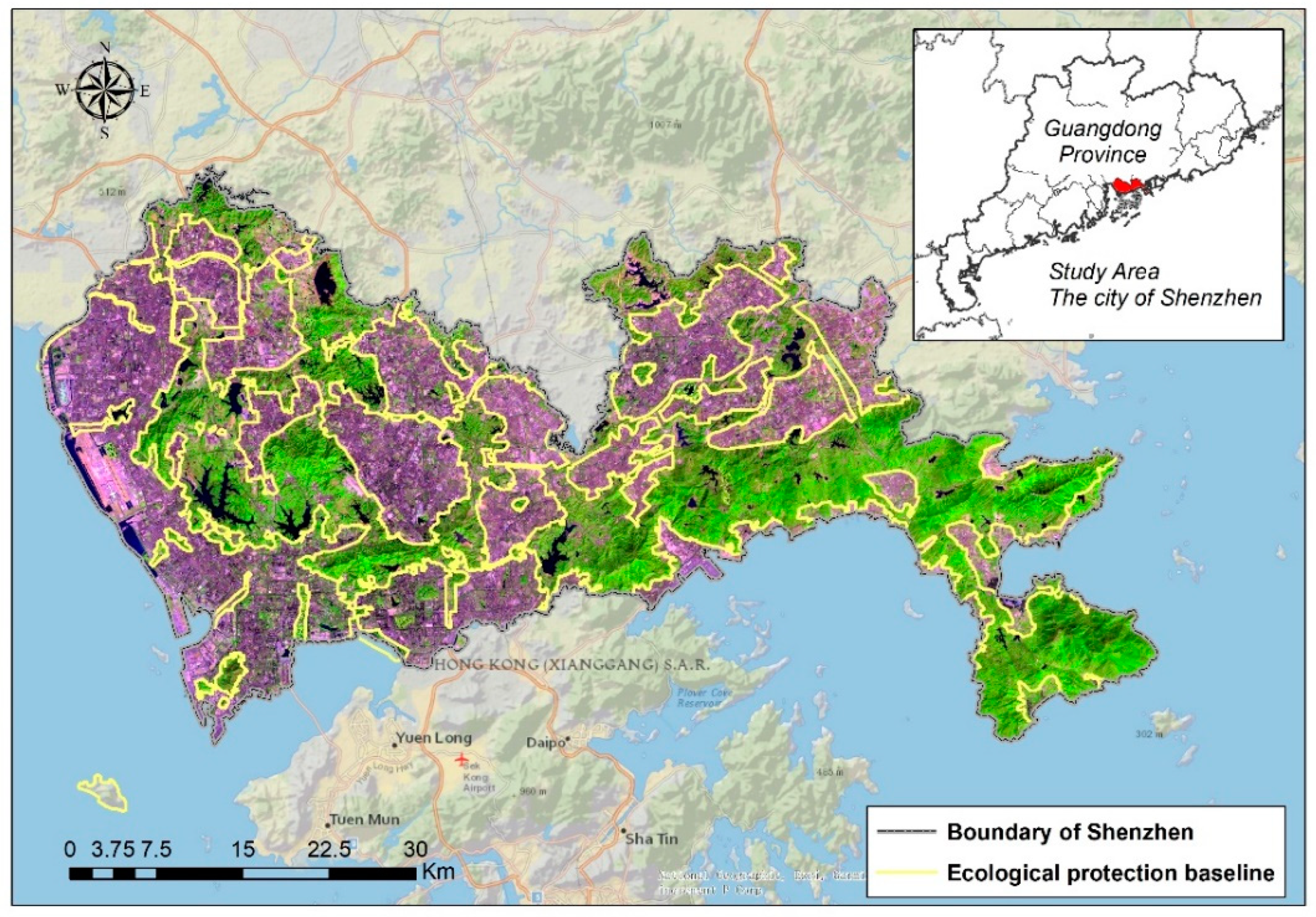
2.1. Study Area

Shenzhen covers an administrative area of 1997 km2, with a population of 13.43 million and GDP of 2692.71 billion RMB in 2019 [47]. Forty years ago, it used to be a village, with only a population of 0.31 million and GDP of 0.2 billion RMB in 1979. Because of the dramatic urban expansion, the size in 2017 was approximately 35 times to that in 1978 and the cover percentage of developed land in 2017 had increased to 48%, which was larger than the together of forest, grass, and cropland, 44% [48]. In order to keep the urban sustainable, the local government released an urban land-use management policy in 2005, among which an ecological protection control baseline is delineated to limit the urban expansion and restore the ecosystem function (Figure 1) [49]. The vegetation coverage of the entire Shenzhen area increased from 48% to 62% in 2000–2018. The forest-cover percentage, in particular, decreased firstly in 2000–2003 and then increased in 2003–2018 [50]. In this study, we defined the areas located outside the ecological protection control baseline as urban built-up areas.

2.2. Aquisition of Time-Series Landsat Imagery

We selected the EVI, a commonly used index and generated from Near-Infrared, Red, and Blue bands of Landsat imagery [51], to quantify the vegetation dynamics. First, the EVI optimized the vegetation signal with improved sensitivity in high biomass regions, and thus can successfully address the saturated signals problem over high biomass conditions that are common for other ratio-based indices [51]. Second, the EVI decouples the canopy background signal and reduces the atmosphere influences by using the atmosphere-sensitive blue band to correct the red band. The calculation of EVI can be found in Equation (1).
EVI = G × ρ N I R + ρ r e d ρ N I R + C 1 ρ r e d C 2 ρ b l u e + L
where ρ N I R , ρ r e d and ρ b l u e are the surface reflectance of the Near-Infrared, Red, and Blue bands which are atmospherically or partially atmospherically corrected. The coefficients C1 and C2 are the aerosol resistance term and L is the adjustment for vegetation canopy background. The values of G, C1, C2, and L adopted in the EVI are 2.5, 6, 7.5, and 1, respectively [52,53].
To maintain the quality and consistency for the time-series observation, the EVI was calculated based on the Surface Reflectance (SR) product derived from the Landsat Level-1 data because the SR product improves comparisons between multiple images over the same region by accounting for atmospheric effects such as aerosol scattering and thin clouds [43]. We selected the Landsat 5 and 7 Surface Reflectance Tier 1 that atmospherically corrected using the LEDAPS and Landsat 8 Surface Reflectance Tier 1 that atmospherically corrected using the LaSRC from GEE. The cloud cover and cloud shadow pixels were excluded using the Quality Assessment (QA) band that integrated into the Tier 1 collection. Because of the relatively low temporal frequency (16-day revisit capability), the number of available clear observations, referring to pixels that are free of cloud, cloud shadow, and snow, is reduced. Such a data preprocessing scheme significantly reduces the reliably representative annual values generated by the image compositing method, such as annual median EVI and monthly maximum EVI, for every year [54]. As a result, we used all the clear observations in 2000–2020, instead of the best-pixel selection, to construct the temporally dense EVI time-series. In this study, a total of 1702 images acquired in 2000–2020 were selected from Landsat 5, 7, and 8. The spatiotemporal variation revealed by the percentage of the clear observations can be found in Figure A1.
Based on the EVI time-series, the unique phenological characteristic of vegetation, represented as a harmonic function with periodical change, can be observed [42]. When the vegetation change occurs, the EVI time-series will be out of the original shape. If the land cover with vegetation converts to other types, the EVI abruptly decreases and the periodical property disappears on the time-series. If the vegetation suffers from diseases, pests, and typhoons, or the vegetation in a pixel partially changes, the inter-annual change reflected by the variation in EVI trends occurs. If the vegetation species changes or the climate condition impacts the vegetation phenology, the periodical property on the EVI time-series changes.

2.3. Change Detection for Urban Vegetation

To investigate the vegetation dynamics from the process perspective, we first detected the timing and frequency of vegetation change by the approach of Continuous Change Detection and Classification (CCDC) [23,42] based on the EVI time-series constructed from the temporally dense Landsat imagery in 2000–2020. The CCDC is a robust approach for monitoring land cover/land-use change and generating maps for any given time using dense time-series satellite imagery. This algorithm contains three components: seasonality, trend, and break. The seasonality corresponds to the seasonal change, mostly caused by the vegetation phenology that is led by seasonal patterns of environmental factors, such as precipitation and temperature. The trend focuses on gradual change, driven by vegetation growth and degradation, climate change, and pests. The break refers to abrupt change, generally caused by land cover change. The study from Zhu et al. (2014) that first presented this approach by input all the Landsat bands to detect the various types of land cover change. Recently, many studies also demonstrated that the CCDC is an adaptive approach in that the single band, such as the NDVI or EVI, can be used to detect the land cover change for a single type [55]. The model of CCDC is shown in Equation (2):
ρ ^ ( i , x ) = a 0 , i + a 1 , i cos ( 2 π T x ) + b 1 , i sin ( 2 π T x ) + c 1 , i x
where ρ ^ ( i , x ) is the predicted value for the i-th band of Landsat at Julian x, a 0 , i is the coefficient for overall value for the i-th Landsat band, a 1 , i and b 1 , i are the coefficients for the intra-annual change for the ith band, c 1 , i is the coefficients for inter-annual change for i-th band, and T is the number of days in one year, which equals to 365.
For each pixel, the CCDC estimated the seasonal, gradual, and abrupt changes for vegetation and recorded the positions of the change occurrence on the EVI time-series. Based on these positions, the CCDC identified the year of vegetation change occurrence and counted the number of the position for quantifying the vegetation change frequency. It has been confirmed that the CCDC is a computationally expensive method and needs huge data storage because it requires a high temporal frequency of clear observation and it updates the time-series model once the new observations are new available [42]. However, benefitting from the powerful computational infrastructure from the GEE, these issues can be addressed and the CCDC algorithm, tabbed as ee.Algorithms.TemporalSegmentation.Ccdc under the Earth Engine algorithms documentation, has been officially released (https://developers.google.com/earth-engine/apidocs/ee-algorithms-temporalsegmentation-ccdc?hl=en, accessed on 10 June 2021). Here, we implemented the CCDC algorithm to detect the vegetation dynamics and lay out the frequency and the latest change year.

2.4. Trends Analysis and Changing Processes Characterization

After detecting the year of change for each pixel, the EVI time-series was segmented into several fragments based on the change year, and the trends in each fragment (also called change period) were calculated by the Ordinary Linear Square (OLS) regression model (Equation (3)). As the change frequency of each pixel is different and the year of change occurrence is time-varying, the duration of each fragment varied in length.
EVI t = a x + b
where a is slope, b is constant, t represents the observation time, and the EVIt is the model estimated EVI value for a pixel at time t.
Based on the trends in each fragment, three kinds of trends, nochange, browning, and greening, respectively assigned as 1, 2, and 3, were identified and the processes of vegetation dynamics can be exhibited from the matrix. For example, if there were two changes, three intervals were segmented and the trends in each fragment were filled in the matrix as shown in Table 1. The class of 123 in the matrix means the process of the vegetation dynamics contains three stages, which change from nochange in the first fragment to browning in the second fragment, and then turning green in the recent period. Here, although all of the pixels had the same investigated period, 2000–2020, each pixel had different numbers of fragments and each fragment had a different duration. As a result, the sub-periods in the process of vegetation dynamics were not fixed. The area proportion of each sub-period can be filled in the matrix to evaluate the how the urban vegetation changes and what the recent status presents. The overview of the integrated approach and its application can be found in Figure 2.

3. Results

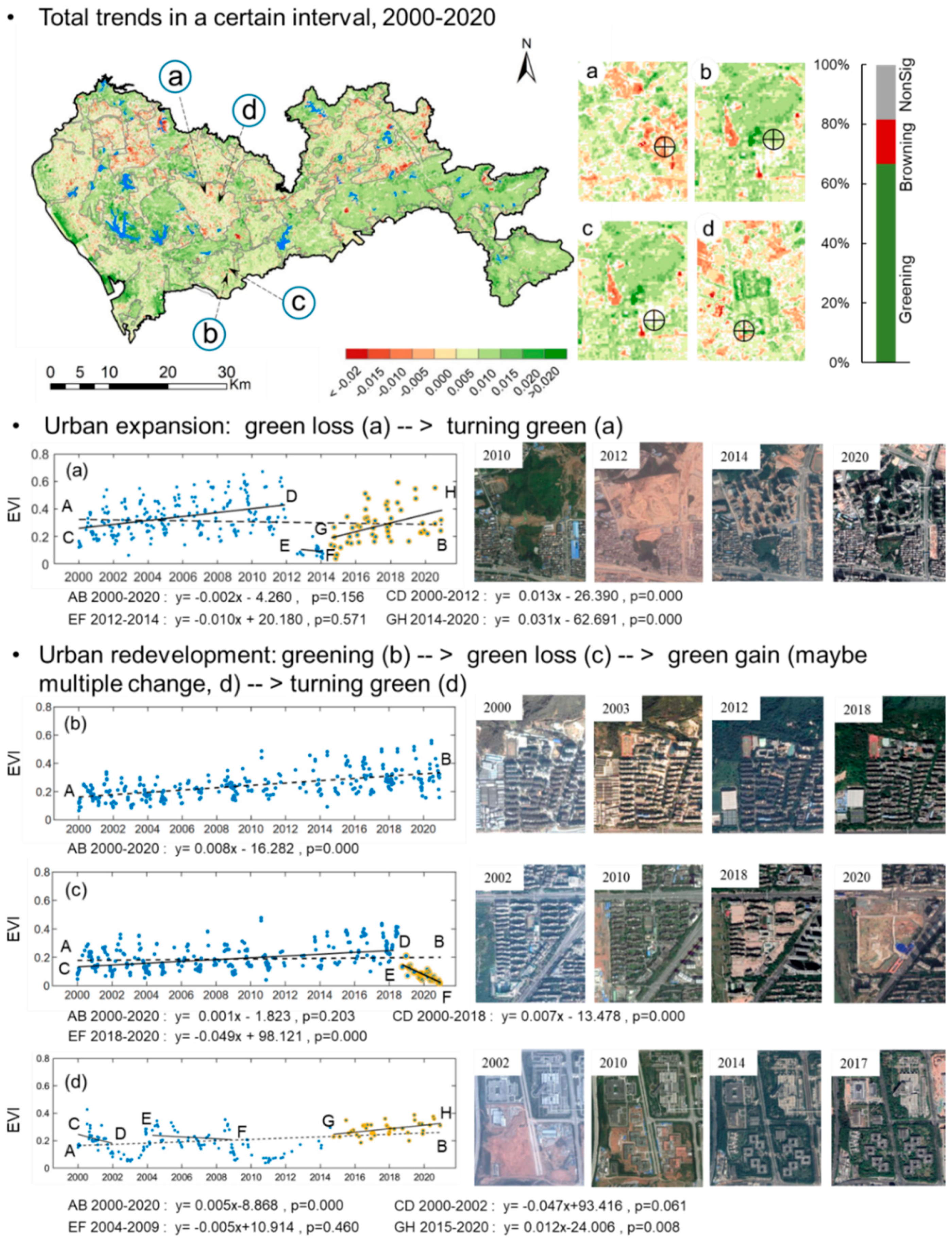
3.1. Non-Monotonous Trends of Vegetation Greenness in the Urban Area

We summarized the vegetation dynamics along with the urban outward expansion and internal redevelopment based on all of the available EVI values calculated from the time-series Landsat imagery in 2000–2020 (Figure 3). The EVI trajectories showed that the vegetation greenness followed the non-monotonous trends and the processes varied from different areas. Such non-monotonous trends were sometimes misleading from the statistical significance and the positive or negative values.
As shown in Figure 3a, the pixel experienced a changing process of urban expansion, in which the EVI abruptly decreased in 2012 and continuously increased in 2014–2020. Although a browning trend was found on Line AB with a slope of −0.002 (p = 0.156), two hidden greening trends, reflected from a positive slope of 0.013 (p = 0.000) in 2000–2012 and another positive slope of 0.031 (p = 0.000) in 2014–2020, were revealed from the process-based analysis.
The changing process of urban redevelopment is summarized in Figure 3b–d, although the EVI values are from different residential areas. When no land cover change occurs and the vegetation continuously grows, a monotonous trend can be simply evaluated. Figure 3b shows a significant increase of the EVI trend on Line AB with a slope of 0.008 (p = 0.000). When a residential/commercial/industrial area is dismantled, an abrupt change occurs on the EVI time-series. Figure 3c shows an insignificant trend presented by Line AB (0.001, p = 0.203) during 2000–2020, while a significantly decreased trend in 2018–2020 was found on Line CD, with a negative slope of −0.049 (p = 0.000). When the residential/commercial/industrial area is redeveloped, the trend will turn green along with the tree replanting. Figure 3d shows a vegetation recovery process, due to which the EVI experienced fluctuant changes of browning and greening, and finally turned green from 2015 with a positive slope of 0.012 (p = 0.008).

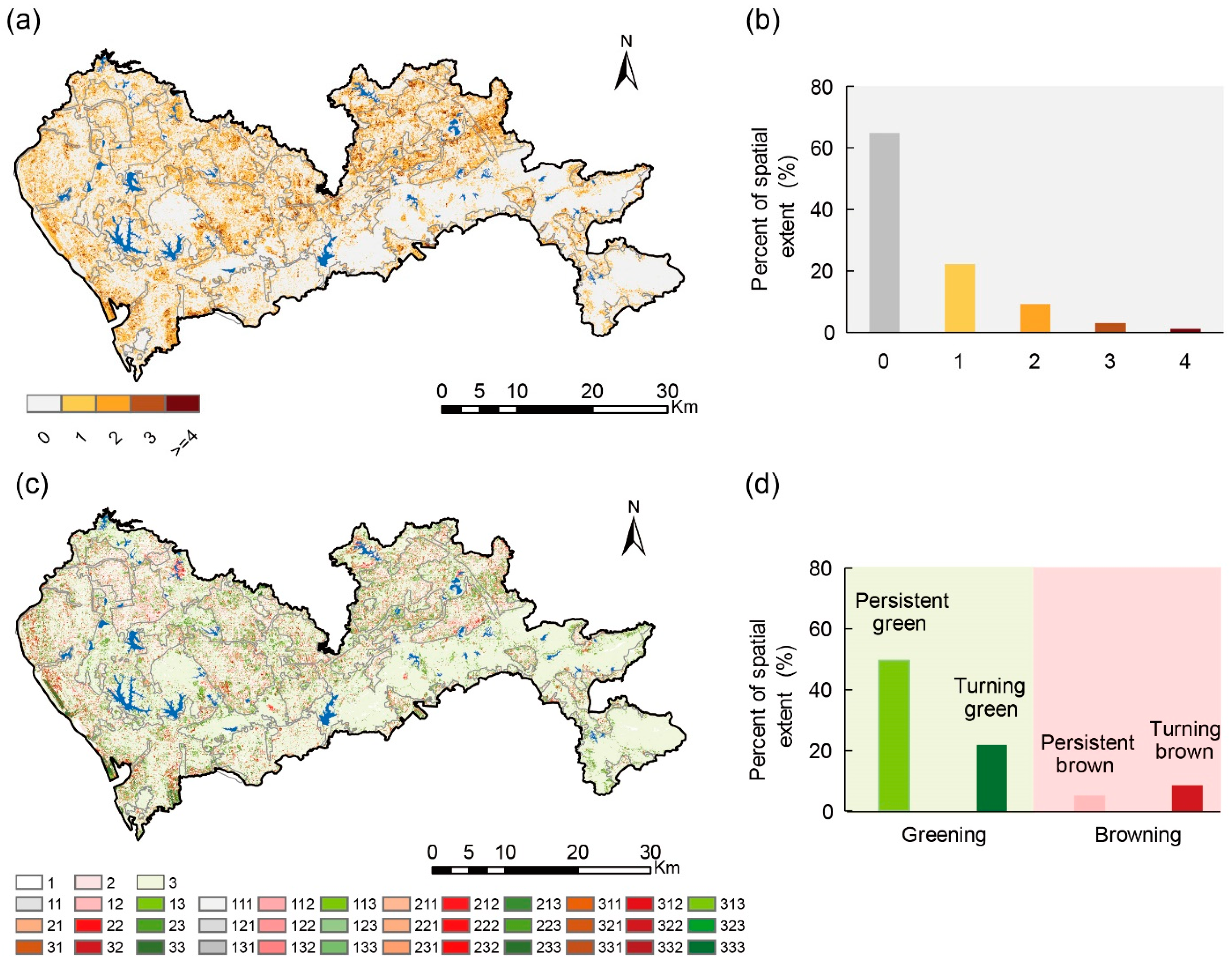
3.2. Spatial Pattern of the Vegetation Dynamics from a Process Perspective

The results of vegetation dynamics from the maps and statistical analysis showed 35.3% of the entire Shenzhen saw at least one-time change and the frequent changes were mostly distributed in the built-up areas, located from the central to the northeast urban areas (Figure 4a,b). Comparing the spatial extents of each level on change frequency, the cover percentages, in order of the change occurrence number, were 22.0%, 9.2%, 3.0%, and 1.1%.
Integrating the trends with dynamics, the statistical results showed 71.2% of all of Shenzhen was greening, among which 49.5% showed consistent trends in greening during the period of 2000–2020 and 21.7% revealed its status of turning green in the recent change period, which began from the latest year of change occurrence detected by the CCDC algorithm to the year of 2020. The results also showed only 13.7% was browning, including 5.2% of persistent browning and 8.5% turning brown. Here, we only display the matrix for the processes of vegetation dynamics with persistence, one-time, and two-time changes caused by land cover, seasonal, and trend changes because their area proportion was over 95%. After summarizing the matrices with one- and two-time changes, three major processes included browning-to-turning green assigned as 23, 123, 223, 233, and 323; no change-to-turning green assigned as 13,113, and 133; and probably turning green assigned as 131 and 231. The areas were 99.0 km2, 108.3 km2, and 20 km2, respectively (Figure 5b,c). It was also found that 106 km2 exhibited green loss, including types of 31, 32, 311, 312, 321, 322, 331, and 332.

3.3. Trends in Recent Change Period for Vegetation Greenness

Focusing on the recent change period, the latest shifts in the trends mostly appeared before 2012, with 66.4% of Shenzhen city with change, indicating a large number of long-term changes occurred in 2000–2020 (Figure 6b). Except for the persistent change, the relatively long-term changes were primarily located in the built-up area, while the short-term changes varied greatly from different areas. The spatial pattern of the latest year of change occurrence showed those short-term changes clustered in four regions, including the western coastal area, central but besides the ecological protection control baseline, the northeast build-up area, and the zone around the northern reservoirs (Figure 6a).
According to the duration of the latest period that starts from the latest year of change occurrence to the year 2020 and the corresponding trends in the latest period, the long-term changes mostly had positive values of EVI slopes and the area proportion of greening in Shenzhen decreased from 2.3% in 2001–2020 to 0.2% in 2019–2020, while the short-term changes showed more insignificant EVI trends with an increased percentage of 0.4% in 2012–2020 to 1.8% in 2019–2020 (Figure 6b). The statistical results of time-varying trends from the boxplot showed those long-term observations had slower change rates. Interestingly, the data distribution of the slopes with positive and negative values were similar, although the amount of them was quite different (Figure 6e,f).

4. Discussion

4.1. The Application of the Temporally Dense Imagery for the Process Identification in Urban Vegetation Greenness

Relatively few studies investigated the urban vegetation dynamics from the process perspective. Our results showed the non-monotonous trends of the vegetation dynamics in urban areas were more complicated because the frequent changes generated several turning points in the EVI time-series, such that the greenness experienced multiple processes (Figure 3 and Figure 4). These multiple processes skewed the trends derived from the linear regression model, misleading the identification of greening and browning via statistical significance and the slope values of trends (Figure 3 and Figure 4). For example, the EVI slope in Figure 3a calculated by the linear regression model exhibited an insignificant decreased trend, with a slope of −0.002. While the process-based analysis showed the vegetation dynamics experienced three stages, including greening in the first stage, insignificant change in the second stage, and greening again in the latest stage, with the slope values of 0.013 (p = 0.000), −0.010 (p = 0.571), and 0.031 (p = 0.000) (Figure 3a). Such effects led by the highly dynamic landscapes, however, can only be improved by the process-based analysis using the temporally dense imagery because the time-series approaches, such as CCDC in this study, segment the EVI time-series into fragments and then evaluate the trends in each sub-period from the piecewise perspective [9,23].
The trends analysis using the temporally dense Landsat data allows more subtle understandings of the urban vegetation change, compared to the composition approach applied to Landsat data that follows a best-pixel selection [56]. As the revisit period of Landsat 5, 7, and 8 was 16 days, the strategy of best-pixel selection, such as annual median EVI or monthly median EVI, will reduce the reliably representative annual value for every year by the Landsat data after removing the cloud cover and cloud shadow pixels. The advantage of the temporally dense data accelerates the detection of structural changes, such as vegetation phenology [57,58] and lake/reservoir shoreline change [59]. The outliers resulting from the simple criteria such as the maximum NDVI or mean NDVI in the growing season based on the time-series can be largely eliminated, which is especially applicable to the regions where the data is frequently absent due to the cloudy and rainy conditions. Additionally, except for the abrupt changes caused by conversions among different land cover types, the inter- and intra-annual changes reflected from the time-series spectral characteristics can only be detected based on the temporally dense imagery [34].

4.2. Process and Recent Trends for the Urban Vegetation Greenness

The information provided from the process analysis, including when the change occurs, how frequently the change happens, and what the changing process experiences, help to better evaluate the vegetation quality and ecosystem function. Compared to most concerns of the vegetation dynamics, including the trends before and after disturbances in forest and grassland, urban ecologists prefer the multiple changes, such as repeated conversions from barren land to grassland in the urban redevelopment process, because the frequent change potentially influences the urban ecosystem properties (e.g. biodiversity and provision of ecosystem services) [26,60,61,62]. The process matrix showed 71.2% (versus 66.7% evaluated from the linear regression model, Figure 3) of Shenzhen was greening, including not only 49.5% of consistent green but also 21.7% of turning green in the latest period. This suggests that the temporal decomposition reveals more information which is frequently ignored and hidden in the total trends quantified by the linear regression model (Figure 5 and Figure 6d). The finding also showed the processes varied greatly even for the greening was found in the latest period (Figure 5). For example, 99 km2 had experienced the process of browning first and then turning green after a period of insignificant change, while 108 km2 had experienced the process of insignificant change first and then turning green. These variations display different stages of urban development, which are beneficial to infer the possible drivers.
The temporally variant trends in the latest change period that starts from the latest change year detected by the CCDC algorithm and ends in the year 2020 exhibit the recent status of vegetation growth and provide opportunities to accurately evaluate the provision of ecosystem services, although the durations varied from different areas (Figure 6). For example, the pixels in the northeast built-up area showed greening in the recent period, suggesting the dwelling environment was improved, although those pixels used to be forest and the urban expansion abruptly decreased the EVI [49]. Such time-varying trends are especially appropriate for the comparison of the ecosystem service provision between the old and new urban areas because the effects of urban outward expansion can be exclusive and can be used to better project the vegetation change.
More importantly, the vegetation dynamics investigated from the process perspective will help government agencies better assess the effectiveness of urban management policies and then implement subsequent planning strategies. The first outcome, change frequency, from the dynamic analysis can be used to evaluate the ecosystem stability. The spatial pattern of change frequency showed the vegetation growth in the eastern area was more stable than that in the western area, although both of them were located inside the ecological protection baseline. When combining the changing process, timing information, and the trends in the recent change period, a large number of dynamics were mostly caused by vegetation recovery after the year 2005 but before 2012, suggesting the previous protection policy, delineating the baseline in 2005, was effective [49]. This forest recovery led to fast greening in a short time interval (Figure 6); the ecosystem continues to function, however, relies on the stability that copes with the obstacles arising from nature and changing environment [63,64]. As a result, how to improve the ecosystem stability, such as increasing the vegetation diversity and making appropriate management schemes, becomes a further consideration for urban planning to achieve the goal of sustainability.

4.3. Limitation and Future Work

In this study, we implemented the CCDC algorithm to detect the vegetation dynamics only based on the EVI time-series constructed from the Landsat SR imagery collection. However, previous studies showed the change detection accuracy will be improved when all of the spectral bands are used as input [42]. Comparing to the Landsat image, the Sentinel-2 data had finer spatial resolution (10 m and 20 m) and temporal resolution (5-day). Additionally, the wavelengths of Sentinel data are more sensitive to the chlorophyll content and phenological states [45,65,66]. It will be more promising when using the Sentinel data to quantify the urban vegetation dynamic. Our results from the process-based analysis showed the Shenzhen city is greening but varies greatly in different areas (Figure 6c,d). Several studies suggested the local climate and the economic input, including irrigation and fertilization, are related to urban greening [31,67], while the economic levels are varied from different regions, which may impact the vegetation greenness. Therefore, more studies need to be performed across many other cities to test and explore the drivers behind urban greenness.

5. Conclusions

This study presented a method that integrates the trends with dynamic analysis and then applied it to investigate the vegetation dynamic from a process perspective in the megacity of Shenzhen by using the temporally dense Landsat imagery. Compared to monotonic trend analysis, this integrated approach has the ability to provide more detailed dynamic information on when and how frequently vegetation change occurs, and what the changing process is. Using the integrated approach, we found that Shenzhen was turning green in 2000–2020, even though a large-scale urban expansion occurred during this period. Nearly half of the city (49.5%) showed consistent trends in greening, most of which were located inside the ecological protection baseline. We also found that 35.3% of Shenzhen experienced at least one abrupt change in vegetation greenness, among which 61.5% of these lands showed trends in turning green in the recent change period. Such information on vegetation greenness, frequently hidden by the trends analysis alone, can be revealed by our approach that integrates the trends with a dynamic process and provides insights for urban vegetation management.

Author Contributions

Conceptualization, W.Y. and W.Z.; methodology, W.Y.; validation, Z.D., J.W. and Y.Q.; writing—original draft preparation, W.Y.; writing—review and editing, W.Z.; funding acquisition, W.Y., W.Z. and W.W. All authors have read and agreed to the published version of the manuscript.

Funding

This research was funded by National Natural Science Foundation of China, grant number 41801178, and 41771203, the Shenzhen Environmental Monitoring Center, grant number SZDL2020335165, and the Shenzhen Municipal Ecology and Environment Bureau, grant number SZCG2018161498.

Institutional Review Board Statement

Not applicable.

Informed Consent Statement

Not applicable.

Data Availability Statement

Not applicable.

Conflicts of Interest

The authors declare no conflict of interest.

Appendix A

Based on the Google Earth Engine platform, the Landsat dataset can be easy to collect and prepare. Here, it needs at least two senses from Landsat to cover the entirety of Shenzhen. A total of 1702 images acquired in 2000–2020 were selected from Landsat 5, 7, and 8 and the available values of every pixel ranged from 446 to 1380. After removing the pixels with cloud cover and cloud shadow, the percentage of clear observations ranged from 15% to 65% (Figure A1).
Figure A1. Spatiotemporal variation revealed by the percentage of clear observations in 2000–2020 acquired from Landsat 5, 7, and 8.
Remotesensing 13 03217 g0a1

References

  1. Shiflett, S.A.; Liang, L.L.; Crum, S.M.; Feyisa, G.L.; Wang, J.; Jenerette, G.D. Variation in the Urban Vegetation, Surface Temperature, Air Temperature Nexus. Sci. Total. Environ. 2017, 579, 495–505. [Google Scholar] [CrossRef]
  2. Van Ryswyk, K.; Prince, N.; Ahmed, M.; Brisson, E.; Miller, J.D.; Villeneuve, P.J. Does Urban Vegetation Reduce Temperature and Air Pollution Concentrations? Findings from an Environmental Monitoring Study of the Central Experimental Farm in Ottawa, Canada. Atmos. Environ. 2019, 218, 116886. [Google Scholar] [CrossRef]
  3. Robinson, S.L.; Lundholm, J.T. Ecosystem Services Provided by Urban Spontaneous Vegetation. Urban. Ecosyst. 2012, 15, 545–557. [Google Scholar] [CrossRef]
  4. Ferrante, G.; Asta, F.; Cilluffo, G.; De Sario, M.; Michelozzi, P.; La Grutta, S. The Effect of Residential Urban Greenness on Allergic Respiratory Diseases in Youth: A Narrative Review. World Allergy Organi. J. 2020, 13, 100096. [Google Scholar] [CrossRef] [Green Version]
  5. Asri, A.K.; Yu, C.P.; Pan, W.C.; Guo, Y.L.; Su, H.J.; Lung, S.C.C.; Wu, C.; Spengler, J. Global Greenness in Relation to Reducing the Burden of Cardiovascular Diseases: Ischemic Heart Disease and Stroke. Environ. Res. Lett. 2020, 124003. [Google Scholar] [CrossRef]
  6. Basner, M.; Babisch, W.; Davis, A.; Brink, M.; Clark, C.; Janssen, S.; Stansfeld, S. Auditory and Non-Auditory Effects of Noise on Health. Lancet 2014, 383, 1325–1332. [Google Scholar] [CrossRef] [Green Version]
  7. Kennedy, R.E.; Cohen, W.B.; Schroeder, T.A. Trajectory-Based Change Detection for Automated Characterization of Forest Disturbance Dynamics. Remote Sens. Environ. 2007, 110, 370–386. [Google Scholar] [CrossRef]
  8. Verbesselt, J.; Hyndman, R.; Newnham, G.; Culvenor, D. Detecting Trend and Seasonal Changes in Satellite Image Time Series. Remote Sens. Environ. 2010, 114, 106–115. [Google Scholar] [CrossRef]
  9. Pan, N.; Feng, X.; Fu, B.; Wang, S.; Ji, F.; Pan, S. Increasing Global Vegetation Browning Hidden in Overall Vegetation Greening: Insights from Time-Varying Trends. Remote Sens. Environ. 2018, 214, 59–72. [Google Scholar] [CrossRef]
  10. Song, X.P.; Huang, C.Q.; Sexton, J.O.; Channan, S.; Townshend, J.R. Annual Detection of Forest Cover Loss Using Time Series Satellite Measurements of Percent Tree Cover. Remote Sens. 2014, 6, 8878–8903. [Google Scholar] [CrossRef] [Green Version]
  11. Fensholt, R.; Rasmussen, K.; Nielsen, T.T.; Mbow, C. Evaluation of Earth Observation Based Long Term Vegetation Trends–Intercomparing NDVI Time Series Trend Analysis Consistency of Sahel from AVHRR GIMMS, Terra MODIS and MODIS and SPOT VGT Data. Remote Sens. Environ. 2009, 113, 1886–1898. [Google Scholar] [CrossRef]
  12. Chen, C.; Park, T.; Wang, X.; Piao, S.; Xu, B.; Chaturvedi, R.K.; Fuchs, R.; Victor, B.; Ciais, P.; Fensholt, R. China and India Lead in Greening of The World through Land-Use Management. Nat. Sustain. 2019, 2, 122–129. [Google Scholar] [CrossRef]
  13. Eklundh, L.; Olsson, L. Vegetation Index Trends for the African Sahel 1982–1999. Geophys. Res. Lett. 2003, 30. [Google Scholar] [CrossRef]
  14. Wu, D.; Wu, H.; Zhao, X.; Zhou, T.; Tang, B.; Zhao, W.; Jia, K. Evaluation of Spatiotemporal Variations of Global Fractional Vegetation Cover Based on GIMMS NDVI Data from 1982 to 2011. Remote Sens. 2014, 6, 4217–4239. [Google Scholar] [CrossRef] [Green Version]
  15. Tucker, C.; Sellers, P. Satellite Remote Sensing of Primary Production. Int. J. Remote Sens. 1986, 7, 1395–1416. [Google Scholar] [CrossRef]
  16. Eklundh, L.; Johansson, T.; Solberg, S. Mapping Insect Defoliation in Scots Pine with MODIS Time-Series Data. Remote Sens. Environ. 2009, 113, 1566–1573. [Google Scholar] [CrossRef]
  17. Zhang, K.; Kimball, J.S.; Nemani, R.R.; Running, S.W.; Hong, Y.; Gourley, J.J.; Yu, Z. Vegetation Greening and Climate Change Promote Multidecadal Rises of Global Land Evapotranspiration. Sci. Rep. 2015, 5, 1–9. [Google Scholar] [CrossRef] [PubMed]
  18. Liang, Z.; Wang, Y.; Sun, F.; Jiang, H.; Huang, J.; Shen, J.; Wei, F.; Li, S. Exploring the Combined Effect of Urbanization and Climate Variability on Urban Vegetation: A Multi-Perspective Study Based on More than 3000 Cities in China. Remote Sens. 2020, 12, 1328. [Google Scholar] [CrossRef] [Green Version]
  19. Wang, X.; Piao, S.; Ciais, P.; Li, J.; Friedlingstein, P.; Koven, C.; Chen, A. Spring Temperature Change and Its Implication in the Change of Vegetation Growth in North America from 1982 to 2006. Proc. Natl. Acad. Sci. USA 2011, 108, 1240–1245. [Google Scholar] [CrossRef] [Green Version]
  20. Nouvellon, Y.; Moran, M.S.; Seen, D.L.; Bryant, R.; Rambal, S.; Ni, W.; Béguéb, A.; Chehbouni, A.; Emmerich, W.E.; Heilman, P.; et al. Coupling a Grassland Ecosystem Model with Landsat Imagery for a 10-Year Simulation of Carbon and Water Budgets. Remote Sens. Environ. 2001, 78, 131–149. [Google Scholar] [CrossRef]
  21. Zhou, W.; Wang, J.; Qian, Y.; Pickett, S.T.A.; Li, W.; Han, L. The Rapid but “Invisible” Changes in Urban Greenspace: A Comparative Study of Nine Chinese Cities. Sci. Total. Environ. 2018, 627, 1572–1584. [Google Scholar] [CrossRef]
  22. Seto, K.C.; Fragkias, M.; Guneralp, B.; Reilly, M.K. A Meta-Analysis of Global Urban Land Expansion. PLoS ONE 2011, 6. [Google Scholar] [CrossRef]
  23. Zhu, Z.; Fu, Y.; Woodcock, C.E.; Olofsson, P.; Vogelmann, J.E.; Holden, C.; Wang, M.; Dai, S.; Yu, Y. Including Land Cover Change in Analysis of Greenness Trends using All Available Landsat 5, 7, and 8 Images: A Case Study from Guangzhou, China (2000–2014). Remote Sens. Environ. 2016, 185, 243–257. [Google Scholar] [CrossRef] [Green Version]
  24. Cohen, W.B.; Yang, Z.G.; Kennedy, R. Detecting Trends in Forest Disturbance and Recovery using Yearly Landsat Time Series: 2. TimeSync–Tools for Calibration and Validation. Remote Sens. Environ. 2010, 114, 2911–2924. [Google Scholar] [CrossRef]
  25. Kennedy, R.E.; Yang, Z.G.; Cohen, W.B. Detecting Trends in Forest Disturbance and Recovery using Yearly Landsat Time Series: 1. LandTrendr–Temporal Segmentation Algorithms. Remote Sens. Environ. 2010, 114, 2897–2910. [Google Scholar] [CrossRef]
  26. Kennedy, R.E.; Andrefouet, S.; Cohen, W.B.; Gomez, C.; Griffiths, P.; Hais, M.; Healey, S.P.; Helmer, E.H.; Hostert, P.; Lyons, M.B.; et al. Bringing an Ecological View of Change to Landsat-Based Remote Sensing. Front. Ecol. Environ. 2014, 12, 339–346. [Google Scholar] [CrossRef]
  27. Filipponi, F.; Valentini, E.; Nguyen Xuan, A.; Guerra, C.A.; Wolf, F.; Andrzejak, M.; Taramelli, A. Global MODIS Fraction of Green Vegetation Cover for Monitoring Abrupt and Gradual Vegetation Changes. Remote Sens. 2018, 10, 653. [Google Scholar] [CrossRef] [Green Version]
  28. Curtis, P.G.; Slay, C.M.; Harris, N.L.; Tyukavina, A.; Hansen, M.C. Classifying Drivers of Global Forest Loss. Science 2018, 361, 1108–1111. [Google Scholar] [CrossRef]
  29. Liu, X.; Huang, Y.; Xu, X.; Li, X.; Li, X.; Ciais, P.; Lin, P.; Gong, K.; Ziegler, A.D.; Chen, A.; et al. High-Spatiotemporal-Resolution Mapping of Global Urban Change from 1985 to 2015. Nat. Sustain. 2020, 3, 564–570. [Google Scholar] [CrossRef]
  30. Wang, J.; Zhou, W.; Wang, J.; Qian, Y. From Quantity to Quality: Enhanced Understanding of the Changes in Urban Greenspace. Landsc. Ecol. 2019, 16, 1145–1160. [Google Scholar] [CrossRef]
  31. Zhong, Q.; Ma, J.; Zhao, B.; Wang, X.; Zong, J.; Xiao, X. Assessing Spatial-Temporal Dynamics of Urban Expansion, Vegetation Greenness and Photosynthesis in Megacity Shanghai, China during 2000–2016. Remote Sens. Environ. 2019, 233, 111374. [Google Scholar] [CrossRef]
  32. Fu, Y.; Li, J.; Weng, Q.H.; Zheng, Q.; Li, L.; Dai, S.; Guo, B. Characterizing the Spatial Pattern of Annual Urban Growth by Using Time Series Landsat Imagery. Sci. Total. Environ. 2019, 666, 274–284. [Google Scholar] [CrossRef]
  33. Corbane, C.; Martino, P.; Panagiotis, P.; Aneta, F.J.; Michele, M.; Sergio, F.; Marcello, S.; Daniele, E.; Gustavo, N.; Thomas, K. The Grey-Green Divide: Multi-Temporal Analysis of Greenness Across 10,000 Urban Centres Derived from the Global Human Settlement Layer (GHSL). Int. J. Digit. Earth 2020, 13, 101–118. [Google Scholar] [CrossRef]
  34. Dara, A.; Baumann, M.; Kuemmerle, T.; Pflugmacher, D.; Rabe, A.; Griffiths, P.; Hölzel, N.; Kamp, J.; Freitag, M.; Hostert, P. Mapping the Timing of Cropland Abandonment and Recultivation in Northern Kazakhstan using Annual Landsat Time Series. Remote Sens. Environ. 2018, 213, 49–60. [Google Scholar] [CrossRef]
  35. Cadenasso, M.L.; Pickett, S.T.A.; Schwarz, K. Spatial Heterogeneity in Urban Ecosystems: Reconceptualizing Land Cover and a Framework for Classification. Front. Ecol. Environ. 2007, 5, 80–88. [Google Scholar] [CrossRef]
  36. Pickett, S.T.A.; Cadenasso, M.L.; Rosi-Marshall, E.J.; Belt, K.T.; Groffman, P.M.; Grove, J.M.; Irwin, E.G.; Kaushal, S.S.; LaDeau, S.L.; Nilon, C.H.; et al. Dynamic Heterogeneity: A Framework to Promote Ecological Integration and Hypothesis Generation in Urban Systems. Urban. Ecosyst. 2017, 20, 1–14. [Google Scholar] [CrossRef] [Green Version]
  37. Woodcock, C.E.; Loveland, T.R.; Herold, M.; Bauer, M.E. Transitioning from Change Detection to Monitoring with Remote Sensing: A Paradigm Shift. Remote Sens. Environ. 2020, 111558. [Google Scholar] [CrossRef]
  38. Li, D.; Lu, D.; Wu, M.; Shao, X.; Wei, J. Examining Land Cover and Greenness Dynamics in Hangzhou Bay in 1985–2016 using Landsat time-series data. Remote Sens. 2018, 10, 32. [Google Scholar] [CrossRef] [Green Version]
  39. Huang, C.Q.; Coward, S.N.; Masek, J.G.; Thomas, N.; Zhu, Z.L.; Vogelmann, J.E. An Automated Approach for Reconstructing Recent Forest Disturbance History using Dense Landsat Time Series Stacks. Remote Sens. Environ. 2010, 114, 183–198. [Google Scholar] [CrossRef]
  40. Li, X.; Zhou, Y.; Zhu, Z.; Liang, L.; Yu, B.; Cao, W. Mapping Annual Urban Dynamics (1985–2015) using Time Series of Landsat Data. Remote Sens. Environ. 2018, 216, 674–683. [Google Scholar] [CrossRef]
  41. Song, X.; Sexton, J.O.; Huang, C.; Channan, S.; Townshend, J.R. Characterizing the Magnitude, Timing and Duration of Urban Growth from Time Series of Landsat-Based Estimates of Impervious Cover. Remote Sens. Environ. 2016, 175, 1–13. [Google Scholar] [CrossRef]
  42. Zhu, Z.; Woodcock, C.E. Continuous Change Detection and Classification of Land Cover using All Available Landsat Data. Remote Sens. Environ. 2014, 144, 152–171. [Google Scholar] [CrossRef] [Green Version]
  43. Zhu, Z.; Zhang, J.; Yang, Z.; Aljaddani, A.H.; Cohen, W.B.; Qiu, S.; Zhou, C. Continuous Monitoring of Land Disturbance Based on Landsat Time Series. Remote Sens. Environ. 2019, 238, 111116. [Google Scholar] [CrossRef]
  44. Gorelick, N.; Hancher, M.; Dixon, M.; Ilyushchenko, S.; Thau, D.; Moore, R. Google Earth Engine: Planetary-Scale Geospatial Analysis for Everyone. Remote Sens. Environ. 2017, 202, 18–27. [Google Scholar] [CrossRef]
  45. Praticò, S.; Solano, F.; Di Fazio, S.; Modica, G. Machine Learning Classification of Mediterranean Forest Habitats in Google Earth Engine Based on Seasonal Sentinel-2 Time-Series and Input Image Composition Optimisation. Remote Sens. 2021, 13, 586. [Google Scholar] [CrossRef]
  46. Dong, Y.; Ren, Z.; Fu, Y.; Miao, Z.; Yang, R.; Sun, Y.; He, X. Recording Urban Land Dynamic and Its Effects during 2000–2019 at 15-m Resolution by Cloud Computing with Landsat Series. Remote Sens. 2020, 12, 2451. [Google Scholar] [CrossRef]
  47. Shenzhen Statistics Bureau. Shenzhen Statistical Yearbook; China Statistics Press: Beijing, China, 2020. [Google Scholar]
  48. Yu, W.; Zhang, Y.; Zhou, W.; Wang, W.; Tang, R. Urban Expansion in Shenzhen Since 1970s: A Retrospect of Change from a Village to a Megacity from the Space. Phys. Chem. Earth Parts A B C 2019, 110, 21–30. [Google Scholar] [CrossRef]
  49. Qian, J.; Peng, Y.; Luo, C.; Wu, C.; Du, Q. Urban Land Expansion and Sustainable Land Use Policy in Shenzhen: A Case Study of China′s Rapid Urbanization. Sustainability 2016, 8, 16. [Google Scholar] [CrossRef] [Green Version]
  50. Song, Y.; Aryal, J.; Tan, L.; Jin, L.; Gao, Z.; Wang, Y. Comparison of Changes in Vegetation and Land Cover Types between Shenzhen and Bangkok. Land Degrad. Dev. 2020, 1–13. [Google Scholar] [CrossRef]
  51. Huete, A.; Didan, K.; Miura, T.; Rodriguez, E.P.; Gao, X.; Ferreira, L.G. Overview of the Radiometric and Biophysical Performance of the MODIS Vegetation Indices. Remote Sens. Environ. 2002, 83, 195–213. [Google Scholar] [CrossRef]
  52. Huete, A.; Justice, C.; Liu, H. Development of Vegetation and Soil Indices for MODIS-EOS. Remote Sens. Environ. 1994, 49, 224–234. [Google Scholar] [CrossRef]
  53. Huete, A.; Liu, H.; Batchily, K.; van Leeuwen, S.J.D. A Comparison of Vegetation Indices over a Global Set of TM Images for EOS-MODIS. Remote Sens. Environ. 1997, 59, 440–451. [Google Scholar] [CrossRef]
  54. Zhu, Z.; Woodcock, C.E.; Holden, C.; Yang, Z. Generating Synthetic Landsat Images based on All Available Landsat Data: Predicting Landsat Surface Reflectance at Any Given Time. Remote Sens. Environ. 2015, 162, 67–83. [Google Scholar] [CrossRef]
  55. Awty-Carroll, K.; Bunting, P.; Hardy, A.; Bell, G. Using Continuous Change Detection and Classification of Landsat Data to Investigate Long-Term Mangrove Dynamics in the Sundarbans Region. Remote Sens. 2019, 11, 2833. [Google Scholar] [CrossRef] [Green Version]
  56. Wulder, M.A.; Loveland, T.R.; Roy, D.P.; Crawford, C.J.; Masek, J.G.; Woodcock, C.E.; Allen, R.G.; Anderson, M.C.; Belward, A.S.; Cohen, W.B.; et al. Current Status of Landsat Program, Science, and Applications. Remote Sens. Environ. 2019, 225, 127–147. [Google Scholar] [CrossRef]
  57. Melaas, E.K.; Friedl, M.A.; Zhu, Z. Detecting Interannual Variation in Deciduous Broadleaf Forest Phenology using Landsat TM/ETM+ Data. Remote Sens. Environ. 2013, 132, 176–185. [Google Scholar] [CrossRef]
  58. DeVries, B.; Decuyper, M.; Verbesselt, J.; Zeileis, A.; Herold, M.; Joseph, S. Tracking Disturbance-Regrowth Dynamics in Tropical Forests using Structural Change Detection and Landsat Time Series. Remote Sens. Environ. 2015, 169, 320–334. [Google Scholar] [CrossRef]
  59. Yao, F.; Wang, J.; Wang, C.; Crétaux, J.F. Constructing Long-Term High-Frequency Time Series of Global Lake and Reservoir Areas using Landsat Imagery. Remote Sens. Environ. 2019, 232, 111210. [Google Scholar] [CrossRef]
  60. Gardiner, M.M.; Burkman, C.E.; Prajzner, S.P. The Value of Urban Vacant Land to Support Arthropod Biodiversity and Ecosystem Services. Environ. Entomol. 2013, 42, 1123–1136. [Google Scholar] [CrossRef]
  61. Lo, A.Y.H.; Jim, C.Y. Differential Community Effects on Perception and Use of Urban Greenspaces. Cites 2010, 27, 430–442. [Google Scholar] [CrossRef] [Green Version]
  62. Zhou, W.; Yu, W.; Qian, Y.; Han, L.; Pickett, S.T.A.; Wang, J.; Li, W.; Ouyang, Z. Beyond City Expansion: Multi-Scale Environmental Impacts of Urban Megaregion formation in China. Natl. Sci. Rev. 2021. [Google Scholar] [CrossRef]
  63. Führer, E. Forest Functions, Ecosystem Stability and Management. For. Ecol. Manag. 2000, 132, 29–38. [Google Scholar] [CrossRef]
  64. Zhou, W.; Pickett, S.T.A.; McPhearson, T. Conceptual frameworks facilitate integration for transdisciplinary urban science. npj Urban Sustain. 2021, 1, 1. [Google Scholar] [CrossRef]
  65. Sothe, C.; Almeida, C.M.d.; Liesenberg, V.; Schimalski, M.B. Evaluating Sentinel-2 and Landsat-8 Data to Map Sucessional Forest Stages in a Subtropical Forest in Southern Brazil. Remote Sens. 2017, 9, 838. [Google Scholar] [CrossRef] [Green Version]
  66. Granero-Belinchon, C.; Adeline, K.; Lemonsu, A.; Briottet, X. Phenological Dynamics Characterization of Alignment Trees with Sentinel-2 Imagery: A Vegetation Indices Time Series Reconstruction Methodology Adapted to Urban Areas. Remote Sens. 2020, 12, 639. [Google Scholar] [CrossRef] [Green Version]
  67. Wellmann, T.; Schug, F.; Haase, D.; Pflugmacher, D. Green Growth? On the Relation between Population Density, Land Use and Vegetation Cover Fractions in a City using a 30-Years Landsat Time Series. Landsc. Urban. Plan. 2020, 202, 103857. [Google Scholar] [CrossRef]
Figure 1. The geographic location of Shenzhen and the Landsat imagery in 2020 (R: SWIR 1 band, G: NIR band, B: Red band). The yellow line represents the ecological protection baseline released in year 2005.
Remotesensing 13 03217 g001
Figure 2. Overview of the approach integrating the trends with dynamic analysis and characterization of the urban vegetation from the process perspective.
Remotesensing 13 03217 g002
Figure 3. Total trends and process of vegetation greenness along with the urban expansion and internal renewal. a shows the process of green loss, green gain, and turning green along with the urban expansion; b, c, and d show different stages in the process of greenness along with the urban redevelopment. The blue filled dot represents the EVI value of one pixel and the yellow dot is the EVI from the latest change period. The historical very high-resolution image is captured from Google Earth.
Remotesensing 13 03217 g003
Figure 4. Spatial pattern of the change incident and process of vegetation change: (a) number of change frequency, (b) percent of each level on change frequency, (c) process of vegetation greenness, and (d) percent of greening and browning.
Remotesensing 13 03217 g004
Figure 5. Matrix for the process of the urban vegetation dynamics. (a) persistent change, (b) process with one-time change, and (c) process with two-time changes. The values in the matrices represent the area proportion.
Remotesensing 13 03217 g005
Figure 6. Spatial and temporal patterns of vegetation change in the recent period. (a) latest change year, (b) trends in the latest change period, (c) EVI slope with persistent change in 2000–2020, (d) EVI slope in the latest changing period, (e,f) data distribution of the EVI slopes in recent change period for greening and browning.
Remotesensing 13 03217 g006
Table 1. Matrix for processes of vegetation dynamics based on the trends in each fragment with different duration.
Status in the Second Fragment Status in the Third Fragment
123
Status in the first fragment11111112113
2121122123
3131132133
21211212213
2221222223
3231232233
31311312313
2321322323
3331332333
Publisher’s Note: MDPI stays neutral with regard to jurisdictional claims in published maps and institutional affiliations.

