Abstract
Equivalent water thickness (EWT) and leaf mass per area (LMA) are important indicators of plant processes, such as photosynthetic and potential growth rates and health status, and are also important variables for fire risk assessment. Retrieving these traits through remote sensing is challenging and often requires calibration with in situ measurements to provide acceptable results. However, calibration data cannot be expected to be available at the operational level when estimating EWT and LMA over large regions. In this study, we assessed the ability of a hybrid retrieval method, consisting of training a random forest regressor (RFR) over the outputs of the discrete anisotropic radiative transfer (DART) model, to yield accurate EWT and LMA estimates depending on the scene modeling within DART and the spectral interval considered. We show that canopy abstractions mostly affect crown reflectance over the 0.75–1.3 m range. It was observed that excluding these wavelengths when training the RFR resulted in the abstraction level having no effect on the subsequent LMA estimates (RMSE of 0.0019 g/cm for both the detailed and abstract models), and EWT estimates were not affected by the level of abstraction. Over AVIRIS-Next Generation images, we showed that the hybrid method trained with a simplified scene obtained accuracies (RMSE of 0.0029 and 0.0028 g/cm for LMA and EWT) consistent with what had been obtained from the test dataset of the calibration phase (RMSE of 0.0031 and 0.0032 g/cm for LMA and EWT), and the result yielded spatially coherent maps. The results demonstrate that, provided an appropriate spectral domain is used, the uncertainties inherent to the abstract modeling of tree crowns within an RTM do not significantly affect EWT and LMA accuracy estimates when tree crowns can be identified in the images.
1. Introduction
The five Mediterranean climate regions (located in California, Chile, South Africa, Australia, and around the Mediterranean Basin) possess a unique biodiversity richness [1,2], including both terrestrial and aquatic ecosystems, despite their limited extent. Supplemented by a favorable climate, with mild and wet winters, these environments saw the early development of many human settlements and civilizations that, in turn, shaped ecosystems through burning, livestock grazing, and agriculture [1,3,4]. Mediterranean vegetation is well adapted to these conditions and can rapidly recover after summer droughts and wildfires.
However, increasing anthropic pressure through both urban and agricultural development and changing climatic conditions is threatening the biodiversity of these ecoregions, so much so that the Mediterranean biome is expected to experience the greatest biodiversity change by 2100 [5]. In particular, as the recent wildfires in California and Australia illustrate, fire risk is likely to considerably increase in the future, with strong impacts on wildlife [6].
Equivalent water thickness (EWT) and leaf mass per area (LMA) are important traits describing of ecosystem processes and functions that can be used to infer essential biodiversity variables [7,8] such as photosynthetic activity and growth rate, and these are recognized indicators of plant health status [9,10,11,12,13]. These traits are also important in fire prevention efforts, as fuel moisture content (FMC) is a common indicator used in fire risk assessment, defined as the ratio between the water content and the dry mass of the vegetation [14,15]. Remote sensing methods can be used to estimate EWT and LMA from hyperspectral images [14,16,17,18,19].
Verrelst et al. [20] defined four different families of methods (parametric empirical-statistical methods, non-parametric empirical-statistical methods, physically based methods, and hybrid methods) used in remote sensing of vegetation, reviewing their respective advantages and drawbacks. Empirical methods, parametric or non-parametric, usually require extensive field data to calibrate models between the hyperspectral reflectance values and the variable of interest and therefore have limited portability to other sensors or sites, as the models are specific to the calibration datasets [21]. They have been extensively used with good success: Cheng et al. [22] demonstrated that EWT maps derived from MODIS images using various vegetation indices (VI) were in agreement with what could be obtained from AVIRIS Classic data, and Dana Chadwick and Asner [23] demonstrated that various leaf biochemical properties, including LMA, could be retrieved from hyperspectral images using partial least-square regressors. Physically based methods rely on the inversion of radiative transfer models (RTM) that simulate canopy reflectance based on model inputs and physical laws. While these methods are able to provide multiple realistic outputs, they are computationally demanding for both database creation and estimations, and their accuracy depends on the level of detail of the modeling within the RTM. Recently, Darvishzadeh et al. [24] demonstrated the ability of LUT-based inversions to estimate leaf chlorophyll content from Sentinel-2 data, with variations in the estimated maps coherent with bark beetle infestation at the site. The last family of methods, designated as hybrid methods, takes advantage of the capacity of RTM to generate realistic reflectances, in order to train scalable and computationally efficient regression models on the simulated databases for subsequent use on hyperspectral images. For instance, using HyMAP imagery, Berger et al. [25] showed that Gaussian process models trained on PROSAIL outputs were appropriate to estimate canopy nitrogen content of crop fields, while Ali et al. [26] illustrated that multiple hybrid methods yield LAI and chlorophyll estimation performances similar to those obtained using LUT-based RTM inversions.
The various RTMs available for physically based and hybrid methods can be roughly categorized into two families. One-dimensional homogeneous models, describing the vegetation as a turbid medium, are the most extensively used [27]. They are easily configurable and fast, at the cost of realism. Three-dimensional heterogeneous models employ ray-tracing methods. These 3D models are highly complex and come at a high computational cost but are much more realistic. These RTMs are more appropriate to model heterogeneous canopies that have a complex architecture, which is all the more important when working at high spatial resolutions. However, due to insufficient field knowledge, trees are often modeled through abstractions, which may lead to inappropriate RTM simulations as these simplifications may affect scene and crown reflectance: Widlowski et al. [28] assessed the effects of omitting or simplifying the woody structure of the trees within DART and found that this could result in a significant bias in the bidirectional reflectance factors (BRF) that increased as the spatial resolution decreased; Ali et al. [29] found that stand height and crown diameter were two of several parameters significantly affecting canopy reflectance; and Janoutová et al. [30] compared the adequacy of various modeling methods in an RTM to lead to realistic spruce crown reflectance. Wocher et al. [19] used a hybrid method to estimate canopy EWT, calibrating their model over PROSAIL outputs: they found that their initial model had to be empirically adjusted to account for radiative effects not modeled in the RTM before providing acceptable results. Overall, making simplifications to model trees or leaves within an RTM may lead to significant reflectance variations over some part of the reflectance spectrum. To what extent does this affect resultant EWT and LMA estimates? Are there spectral ranges that remain mostly unaffected by the abstractions? These issues are of great importance to design methods to estimate EWT and LMA at sites with little a priori information and that could be generalized to sites belonging to the same ecosystem type.
The objective of the present study was to evaluate the effect that tree modeling abstractions within an RTM have on crown reflectance (i) to identify spectral ranges that are not very sensitive and (ii) to assess these findings by training machine learning models on RTM-generated data to estimate EWT and LMA. The DART model [31,32] is a typical 3D RTM that allows for various levels of detail in the modeling and was therefore chosen for the present study. To do so, a preliminary analysis was done using synthetic images to compare the performances of various model runs within an RTM and to serve as reference, followed by a real case study involving two different Mediterranean climate sparse forests. EWT and LMA accuracies were estimated and assessed by comparing estimated values to field measurements, and their consistency was validated using the results from the synthetic analysis.
2. Materials and Methods
2.1. Study Sites and In Situ Validation Data
The study sites are grass-oak pine woodlands located in the lower foothills of the Sierra Nevada Mountains (Tonzi Ranch (TZ), latitude: 38.5°N; longitude: 121.0°W, San Joaquin Experimental Range (SJER), latitude: 37.1°N; longitude: 119.7°W). They both have a Mediterranean-type climate with hot, dry summers and mild, wet winters and are respectively located at about 200 m and 350 m above sea level. The overstory of TZ is dominated by blue oaks (Quercus douglasii—QUDO), while SJER presents a mix of QUDO and interior live oaks (Quercus wislizeni—QUWI). The pine species at both sites is the gray pine (Pinus sabiniana—PISA). QUDO are deciduous and active from April to November, while QUWI and PISA are evergreen.
The understory is composed of annual grass species active from December to May and dry during the summer period. TZ presents a stem density of 144 ha, an average LAI of 0.8 m/m, and a mean canopy cover (CC) of 47% [33]. Mean annual temperatures and precipitations are 16.5 °C and 562 mm, respectively, and the soil is an Auburn very rocky silt loam. Concerning SJER, the canopy cover is around 30%, with an average temperature and annual precipitations of 16.5 °C and 485 mm, respectively. The only soil type at SJER is a Vista rocky coarse sandy loam [34].
Figure 1 shows aerial views of the sites as well as the location of the field measurements used in this study. Table 1 shows the main dimensions of the trees present on both sites.
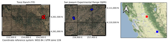
Figure 1.
Aerial view of Tonzi Ranch (red markers) and San Joaquin Experimental Range (blue markers). Location of the trees where leaf collection took place is indicated by the colored markers.

Table 1.
Crown characteristics of the QUDO and QUWI trees obtained from a field survey over the two sites. In parentheses, the number of tree measurements used to compute the statistics.
To retrieve EWT and LMA, fully expanded leaves were collected from healthy QUDO and QUWI individuals presenting a structure typical of the site. Leaves were collected from the upper, sunlit portions of the canopy within an hour of the AVIRIS-Next Generation (AVIRIS-NG) overflights. Samples were obtained from branches on the east and west sides of the trees, and specific attention was paid to ensure that collected leaves were healthy. For both sites, leaf collection occurred during dry days. Once collected, leaves were placed in a plastic bag and stored either on blue ice or in a lab refrigerator until lab measurements could be made (within less than 48 h). Plastic bags had been weighed with a milligram precision scale before going to the field. In the lab, the bags with leaves inside were weighed, and leaf fresh weight was computed as the difference between full and empty bags’ weights. All leaves were scanned in TIF format with 150 dpi. Leaf area was estimated using the scanned image using TOASTER software. Finally, all the leaves were put into a paper bag to dry at 65 °C until the weight did not change when the leaves were reweighed (two to three days) to obtain leaf dry weight. Finally, EWT and LMA were calculated according to Equations (1) and (2) [15]. Table 2 presents the characteristics of the field data obtained for EWT and LMA.
Table 2.
Field data collected over TZ and SJER at the time of the AVIRIS-NG flights for QUDO and QUWI.
Reflectance measurements for ground types and tree trunks took place on both TZ and SJER with an Analytical Spectral Device (ASD; ASD Inc., Boulder, CO, USA). A spectralon panel served for calibration before each acquisition. Different soil types were measured so as to ensure that the spatial variability of both sites was taken into account. These ground types included, but were not limited to: PISA litter, QUDO litter, and mixed dry herbaceous layer (see Figure 2 for illustrations of the various ground types considered in this study). Trunk bark reflectances were obtained from portions of the trunks collected and put on a horizontal surface to facilitate the measurements. All reflectances were obtained over the 0.350–2.500 m spectral range.
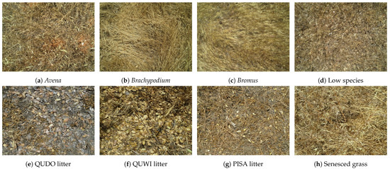
Figure 2.
Illustration of the various ground types that were encountered and used for background spectra measurements.
Figures (a–d) were taken on TZ, while Figures (e–h) were taken on SJER.
2.2. Trunk and Branches Structure
Terrestrial lidar scans were acquired for a number of sites at each of the locations. The Compact Biomass Lidar (CBL) [35], developed in-house at the University of Massachusetts Boston, was used to obtain 4 scans around each tree area. The lightweight, robust, and rapidly scanning CBL utilizes a commercial 905 nm SICK LMS-151 lidar on a motorized rotary table, acquiring a point cloud of the 270° enveloping the instrument out to a maximum of 40 m, with a point cloud of first and second returns at a 0.25° resolution and with a 0.86° beam divergence.
Point clouds were coregistered using CloudCompare 2.6.3.1 (www.cloudcompare.org, accessed on 23 July 2019), and several trees were isolated and trimmed so that the majority of the remaining points originated from the woody structure. Trimming was done in two steps: first, a statistical outlier removal filter was applied, as the points corresponding to foliage followed no structure; then, connected components were segmented, and those visually corresponding to foliated parts of the tree were manually removed. The point clouds were then processed using TreeQSM v2.3.0 (Raumonen et al. [36], doi:10.5281/zenodo.844626) to generate a 3D woody structure through fitting of multiple circular cylinders, up to the fourth order of branches when possible. Six different woody structures were reconstructed for QUDO and were assumed to be representative of the non-photosynthetic vegetation (NPV) of both QUDO and QUWI trees. One of these woody structures is shown in Figure 3 as an example.
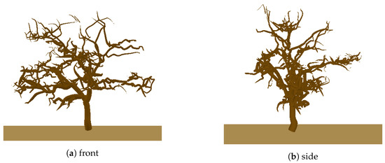
Figure 3.
Illustration of one of the tree non-photosynthetic structures obtained from the lidar
acquisitions.
2.3. Airborne Hyperspectral Remote Sensing Data
AVIRIS-NG hyperspectral data are acquired, processed, and provided by NASA Jet Propulsion Laboratory. The sensor has 432 spectral bands and a full width half maximum of 0.005 m from 0.380 to 2.510 m. Airborne acquisitions took place on 6 June 2014 at 11h24 Pacific Standard Time (PST) over TZ, and on 11 June 2014 at 13h00 PST over SJER. The ER-2 aircraft flew close to noon to avoid spectral directional effects. Preprocessing steps provided by NASA JPL included radiometric calibration, geometrical orthorectification, and atmospherical correction performed with ATREM [37], to retrieve surface reflectance values. The spatial resolution of the hyperspectral images was 2 m.
2.4. Classification of Conifers and Broad-Leaved Trees
Since this study only focuses on broad-leaved trees, a species classification was needed as a first step. A support vector machine (SVM) method was used to classify the tree types (broad-leaved and conifer) present on both sites in the AVIRIS-NG images. For TZ, 506 and 557 pixels were manually selected for the broad-leaved and conifer classes, respectively, while for SJER, 833 and 412 pixels were selected, based on field inventories, tree structural information derived from LiDAR data (crown height) collected in 2009 (PISA sample height assumed to be higher than 20 m for TZ, as per Kobayashi et al. [38]), and visual inspection. Concerning SJER, more pixels were selected for broad-leaved than for conifers to account for both QUDO and QUWI. The SVM was run with the radial basis function kernel (C: 6.5; : 0.0055). Over 20% of the data were used as test set, and accuracy scores were 93% and 96% for TZ and SJER, respectively, so it was decided not to optimize the hyperparameters further. The resulting classification maps were also visually compared to true-color aerial images of the site, as PISA have a visually distinct color from both QUDO and QUWI, in order to further confirm classification accuracy.
2.5. Radiative Transfer Modeling
DART 5.7.8 model was used to simulate canopy reflectances. DART is a Monte Carlo 3D RTM capable of simulating light interactions and multiple scattering effects within any natural or urban 3D scene, taking into account the topography and the atmosphere. A detailed description of the DART model can be found in Gastellu-Etchegorry et al. [31] and Gastellu-Etchegorry et al. [32]. Trees are defined by various structural parameters such as the crown dimensions and location or the distribution and optical properties of the leaves. The reliability of DART as a 3D RTM has been demonstrated in several studies, notably during its participation in the RAMI experiments [39,40,41,42]. Leaf optical properties were simulated within DART using the PROSPECT-D [43] version of PROSPECT [44]. Unless stated otherwise, the sampling scheme for every DART and PROSPECT parameter was done according to a Latin hypercube, and the DART pixel size was 40 cm.
DART was used to generate a synthetic hyperspectral image of a sparse forest, and multiple databases were subsequently used to trained random forest regressors (RFR). These databases are detailed in the following sections:
- Section 2.7, for the sensitivity analysis:
- –
- SFR–Reference database, with a simplified forest representation (SFR) serving as reference;
- –
- variation database, with the variation cases.
- Section 2.8, to train the RFR dedicated to the synthetic image:
- –
- SFR database, with an SFR modeling;
- –
- DETAIL database, with a detailed modeling.
- Section 2.8, to train the RFR dedicated to the AVIRIS-NG images:
- –
- TZ database, with an SFR modeling, dedicated to TZ;
- –
- SJER database, with an SFR modeling, dedicated to SJER.
2.6. Synthetic Image Generation
The use of synthetic images for this study was driven by two main reasons: (i) to overcome the insufficient field validation data available for this study by adding synthetic validation data, and (ii) to give an idea of the estimation performances under controlled conditions, e.g., when all the field data are available to properly configure the RTM, and how the performance degrades with incomplete modeling.
The synthetic forest scenes were procedurally generated in DART. To do so, trees whose characteristics (tree height, crown diameter, tree leaf area index (LAI), leaf biochemical content, trunk and branches 3D model) were randomly determined were placed over a 240 × 240 m area such that the tree crowns did not overlap, until either the CC reached 50% or no tree could fit in anymore—whichever came first. To avoid crown overlap due to the scene repetition done by DART, no tree was present in a 20 m band on the edges of the scenes. Tree crowns were modeled as cylindrical for the lower two thirds, and with a half sphere for the upper third, with 60% empty crown voxels, corresponding to the upper boundary of empty voxels within the tree crown in the sensitivity study done by Ferreira et al. [45]. The vertical profile of tree LAI (ratio of the sum of the upper surfaces of the leaves over the projected surface of the crown) distribution within the crown depended on elevation: crowns were divided into three equal-sized parts (bottom, middle, and top), and each part’s LAI was multiplied by a weighting factor depending on the average height of each part. These weighting factors were obtained by computing a leaf area density for each part following the relationship found by Béland et al. [46] for oak trees and normalizing these densities so that their sum equals 1. Tree LAI corresponded to those that can be found in the literature concerning the blue oaks of Tonzi [47]. The understory was modeled using a heterogeneous Lambertian surface for the soil and a 3D dry grass layer with an LAI of 0.7 m/m, similar to what can be found over the Tonzi Ranch site [38,48]. Sun elevation was set to 75°, which roughly corresponds to the solar elevation at noon at the latitudes of TZ and SJER in June (and the time of the AVIRIS-NG overpasses). The atmosphere was configured for mid-latitude summers, and aerosols were set to rural, summer mid-latitudes with a visibility of 23 km. Table 3 gives a summary of both overstory and understory characteristics.
Table 3.
Overstory and understory characteristics used for the procedural generation of the synthetic scenes within DART.
After generation of reflectance image, it was downsampled to 2 m by pixel aggregation to attain the same ground sampling distance (GSD) as AVIRIS-NG. An example of the modeling of an isolated tree and a top view of the synthetic scene before and after the downsampling are shown in Figure 4.
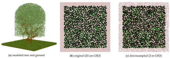
Figure 4.
Example of the scene modeling and colored compositions of the procedurally generated 240 × 240 m2 scene.
The spatial downsampling was done by spatial aggregation and averaging of the pixels.
2.7. Reflectance Sensitivity to Structural Elements
Before generating the training databases for the RFR, a monovariant sensitivity analysis was done to assess reflectance differences between the tree crowns modeled in DART with and without various detailed structural elements. To do so, reflectance values were extracted from the within-crown pixels and averaged. The reference DART modeling for the structural sensitivity was an SFR, with four lollipop trees placed over a Lambertian ground surface so that the scene bidirectional reflectance factor (BRF) was the closest to that of a forest [49]. This simple modeling is based on the work done in Gascon et al. [50], Banskota et al. [51] and Miraglio et al. [52]. The leaf angle distribution was set to ellipsoidal, so that the average leaf angle was a variable parameter. The solar elevation angle was set to 75°.
The reflectance changes due to the introduction of five refined structural elements in the SFR scene were evaluated over the 0.75–2.4 m range, for which EWT and LMA have the most influence on the reflectance [53]. The tested structural elements are indicated in Table 4. The tested canopy height corresponded to the case where tree height was one standard deviation above the average. To ensure that results were not specific to a single combination of LAI, average leaf angle (ALA), and leaf biochemical content, reflectance changes were measured for 1000 combinations (see Table 5 for the variation ranges of each variable).
Table 4.
Structural elements and their variation that were considered as model inputs for the sensitivity analysis.
Table 5.
DART and PROSPECT fixed and variable parameters used to generate the various databases used in this study.
2.8. Random Forest Regressors
In order to assess the best performances that could be obtained by RFR when estimating EWT and LMA over high resolution hyperspectral images, and to understand how these performances were affected by the RTM parametrization, two different training databases were built for estimation purposes over the synthetic images.
The first database, designated as the SFR database, used a simplified forest representation using DART. Therefore, only the mean tree height, height below crown, and crown diameter structural components were considered for modeling purposes. The leaf angle distribution (LAD) was set to ellipsoidal, and the Lambertian ground reflectance was extracted from the open parts of the synthetic images. This is a model that is realistically achievable and has been successfully used to estimate biophysical and biochemical parameters [50,52].
The second database, designated as the DETAIL database, used a very detailed 3D modeling, including all the structural elements used during the building of the synthetic scenes. Ground and tree crowns were modeled as in the synthetic images, using detailed 3D non-photosynthetic vegetation (NPV). Three different tree heights were considered, following the height distribution within the images. Such a precise parametrization, while not realistically feasible on real cases due to insufficient field information, was accomplished here to serve as a reference for the best performance that can be expected from RFR.
For estimations over the two AVIRIS-NG images, two different training databases were built following the specificities of each site. A simplified forest representation was used in each case, taking into account the results presented in Section 3.2 for the synthetic images. Indeed, there was no difference in terms of estimate accuracy over the synthetic image between an RFR trained with the DETAIL database over the 0.75–2.4 m range and one trained with either the SFR or DETAIL database over the 1.5–2.4 m range. To take into account the various understory types present on the sites, it was decided that the ground would be modeled as a Lambertian surface but with varying reflectance values derived from the background spectra obtained in the field (see Section 2.1). Since the specific crown shape and leaf distribution within the crown were unknown, crowns were modeled as homogeneous ellipsoids with varying ALA, similar to what was done for the synthetic image.
Each database comprised 5000 entries, generated according to Table 5. The variation ranges considered for EWT and LMA were set such that they would encompass more than the field values given in Table 2 and reduce the overfitting when training the RFR for TZ and SJER. Similarly, the LAI variation range was set so as to encompass more than the tree LAI field measured values by Karlik and McKay [47]. Indeed, all DART scenes were designed so that the CC was 40%, the relationship between LAI and tree LAI therefore being . Therefore, a LAI range of 0.3–4 m/m leads to a tree LAI range of 0.75–10 m/m, wider than the 2.5–7.7 m/m reported by Karlik and McKay [47]. Variable parameters were sampled following a Latin hypercube sampling. For each case, reflectances from the pixels comprised within the tree crowns were extracted from the DART images, averaged, and linked with their respective EWT and LMA values to build the various databases. All reflectances were noised using a multiplicative wavelength-independent noise and an additive wavelength-independent noise as such:
with the noised reflectance and R the RTM-computed reflectance.
Random forest regressors require a number of hyperparameters to tune them, such as the number of trees, features to consider at each split, number of levels, etc. For all the RFRs used in this study, bootstrapping was used, and all features were considered at each split. The tuning of the other hyperparameters was done through a randomized search with 150 iterations and 3-fold cross validation over the grid defined in Table 6. RFRs were trained using different spectral intervals. Two cases were tested: using information from the full 0.75–2.4 m range, corresponding to the spectral ranges affected by EWT and LMA [53], or only using the spectral information from the 1.5–2.4 m range. Seventy percent of the databases were used for training, the remaining 30% serving as test data. RFRs were trained on the average tree crown reflectances and their associated EWT or LMA values.
Table 6.
Values of the RFR hyperparameters considered in the randomized search for the optimal combination.
For the synthetic images, the position of trees and leaf biochemical content was perfectly known. Therefore, the estimated EWT and LMA contents of each vegetation pixel were directly compared to the true values by averaging estimates done over each crown. Performance estimates were assessed using both root-mean-square error (RMSE) and R. On the other hand, for the AVIRIS-NG images, because of some degree of uncertainty inherent in GPS measurements, registration of the images, and the difficulty in delineating exact tree crowns, the exact crown pixels to be associated with the validation data were not known. To overcome this, it was decided to compare the validation values with the average of estimated values over a window of 5 × 5 pixels centered on the GPS locations of the trees. Estimation performances were also assessed using RMSE and R, although R results are difficult to discuss as the number of validation data and their variation ranges are limited.
3. Results
3.1. Effects of Structural Elements on Crown Reflectance
The sensitivity analysis shed light on the influence of the various structural modeling parameters on tree crown reflectance (see Figure 5a). Three-dimensional NPV, proportion of empty voxels, and canopy height affected crown reflectance in a similar fashion, lowering reflectance by about 0.02 over the 0.75–1.3 m spectral range while barely affecting the 1.5–2.4 m range. Conversely, changing crown shape and LAI distribution within the crown (detailed crown scenario) led to an increase in reflectance over the 0.75–1.3 m range but barely any change at longer wavelengths. Understory modeling did not affect reflectance significantly. Overall, the introduction of 3D NPV had the most effect on crown reflectance: more than 50% of the cases had variations exceeding 0.02, with a standard deviation of about 0.015, the highest among the structural elements. Analyzing the relative variation in reflectance, shown in Figure 5b, it appears that for wavelengths longer than 1.5 m, more than half of the sensitivity cases presented reflectance variations below 5%, a typical uncertainty associated with high calibration efforts [28]. Still, the 3D NPV, empty voxels, and canopy height scenario all showed relative variations greater than 5% for at least 25% of the sensitivity database, highlighting the importance of the various tree structural elements on the crown reflectance computed by DART.
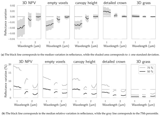
Figure 5.
Crown reflectance variations caused by the introduction of more detailed structural elements during the monovariant
sensitivity analysis over the 1000 tested cases.
To further analyze the results for the 3D NPV case, an analysis of variance (ANOVA) of crown reflectance variations was done at 1.1 m, 1.7 m, and 2.05 m to assess which of the traits (LAI, LMA, EWT, N, ALA) was responsible for them. The results of the ANOVA are presented in Table 7. At 1.1 m, only LMA values were driving the variance, with p values clearly below 0.05 (<10). At 1.7 m, LMA was still the main driver of variance, although at this wavelength, the effects of LAI and EWT were also non-negligible, with p values of , , and , respectively. It is at the 2.05 m that all vegetation traits except N had a significant influence, LAI and EWT being the most important drivers.
Table 7.
p Values of each vegetation trait obtained from the ANOVA on crown reflectance variations.
3.2. EWT and LMA Estimations
Figure 6 shows how the databases generated with DART in forward mode compare with the crown reflectances from the hyperspectral images. For the synthetic image, crown reflectances were within database boundaries for both SFR and DETAIL over the whole 0.75–2.4 m. The effect of the detailed structure on database reflectances was clearly visible over the 0.75–1.3 m spectral range, with reflectances from the DETAIL database being noticeably lower than those from the SFR database and showing overall a larger dispersion. For the TZ and SJER databases, dedicated to the AVIRIS-NG images and generated with an SFR modeling, it appeared that the spectral behavior of the tree crowns over the 0.75–1.2 m range was not well captured, with an overestimation of the reflectance by DART. However, over the 1.5–2.4 m range, crown reflectances were well within database boundaries and could therefore be considered appropriate to train the RFR.
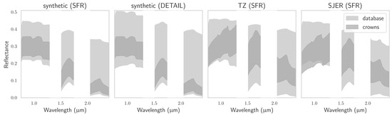
Figure 6.
Reflectance spectra contained within the various databases and the reflectance spectra of the broad-leaved trees
present within the associated hyperspectral images.
Table 8 presents the RMSE and R values of the trained RFR predictions when applied over the train, test, and application sets for the synthetic forest image. For all databases, dedicated to the synthetic or AVIRIS-NG images, training and testing accuracies were consistent. Over the training datasets, RMSEs were about 0.0011 g/cm and R> 0.95 for both EWT and LMA, while over the testing datasets, performances slightly degraded, with RMSE around 0.0025 g/cm and R close to 0.90. Concerning the synthetic images, it appeared that the spectral intervals used to train the RFR, either 0.75–2.4 m or 1.5–2.4 m, did not affect performances on the train and test databases. The feature importance values identified by each RFR after training are presented in Appendix A.
Table 8.
Performances of the RFR dedicated to the synthetic scene when applied over the trained and test sets as well as over the hyperspectral images.
Over the hyperspectral images, however, performances differed depending on the spectral interval. Indeed, when trained over the whole spectral range, LMA estimates were significantly less accurate with an SFR model, with an RMSE of 0.0035 g/cm compared to DETAIL’s 0.0021 g/cm RMSE. Accuracy concerning EWT was unaffected by the model. Restricting the training to wavelengths longer than 1.5 m made the SFR scenario perform significantly better, with an RMSE of 0.0019 g/cm, equal to the DETAIL scenario. For the synthetic image, accuracy estimates were in line with those obtained over the test sets. The estimators dedicated to the AVIRIS-NG images also presented performances similar to those obtained over the test datasets, with the former having an RMSE of 0.0029 and 0.0028 g/cm for LMA and EWT, and the latter having an RMSE between 0.0030 and 0.0033 g/cm for these traits. Figure 7 presents the estimated EWT and LMA values and how they compare with the reference values over the synthetic and AVIRIS-NG images.
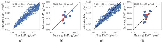
Figure 7.
Comparison between LMA and EWT estimated and true/measured values over the (a,c) synthetic and (b,d)
AVIRIS-NG images. Marker colors concerning the AVIRIS-NG images refer to the study sites: red for TZ, blue for SJER.
Figure 8 shows EWT and LMA estimation maps over the broad-leaved trees of the two study sites. Estimated values within tree crowns did not vary much, indicating that they are not random. At both sites, the zones with the highest tree density were also the zones with the highest EWT and LMA.
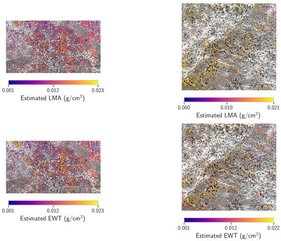
Figure 8.
EWT and LMA estimation maps from the AVIRIS-NG hyperspectral images acquired over the two study sites (left: TZ; right: SJER).
4. Discussion
4.1. On the Use of Synthetic Images
This study complemented the limited field measurement dataset with synthetic forest scenes generated within DART. The DART model took part in the four phases of the RAMI model validation experiments [41], which showed that the simulation results of six 3D Monte Carlo models (including DART) were consistently in good agreement and could therefore be used to generate surrogate truth data for later RTM performance assessment. Synthetic scenes generated with DART have previously been used to calibrate vegetation indexes [54], to assess the sensitivity of a biomass prediction method [55], and DART is regularly used for the estimation of various biophysical and biochemical parameters. While, obviously, synthetic scenes do not fully replace real hyperspectral acquisitions, the consistency that the truth data produce as compared to field data should make them acceptable surrogates for validation purposes, provided sufficient modeling realism has been achieved.
4.2. Influence of the Structural Parameters on Crown Reflectance
The field work presented in Section 2.1 and Section 2.2 allowed for modeling realistic trees in the DART model, in particular by taking into account the structure of the non-photosynthetic elements of the trees. It was thus possible to evaluate the variation in reflectance of scenes with different levels of modeling abstraction. The sensitivity analysis, whose results are presented in Section 3.1, demonstrated that most abstractions done as part of the SFR scenario could significantly influence crown reflectance over the 0.75–2.45 m spectral range, in particular over the 0.75–1.5 m range, with more than 50% of the cases of the 3D NPV scenario exceeding the 5% uncertainty threshold considered by Widlowski et al. [28]. Some of the variations in crown reflectance found in the sensitivity analysis were in line with what was previously obtained in the literature. Ferreira et al. [45] and Malenovský et al. [56] have shown that the presence of NPV within the tree crown (in the form of a turbid medium with branch optical properties) significantly affected reflectance over 0.7–0.9 m and dampened the red-edge, especially for the sunlit portions of the crowns. The results related to the proportion of empty voxels within tree crowns also corroborated what was obtained by Ferreira et al. [45] that at shorter wavelengths, for pixels that were completely filled by the tree crowns, it produced higher reflectance values than those without, due to increased within-crown scattering leading to more radiance leaving the crown. It appears that these model parameters still significantly affect crown reflectance in the short-wave infrared.
Even for wavelengths longer than 1.5 m, this 5% uncertainty threshold was exceeded for the scenarios 3D NPV, empty voxels, and canopy height for more than 25% of the (LAI, EWT, LMA, N, ALA) combinations tested. However, the ANOVA results presented in Table 7 show that the reflectance variation in the various scenarios depended on the values of the vegetation traits. Moreover, the relative quantity of variance explained by each trait depended on the spectral band. This is significant: if reflectance variations due to a certain level of abstraction depend on vegetation traits in the forward mode, it means that the abstraction will lead to uncertainties regarding the trait estimations in inverse mode.
Therefore, considering wavelengths shorter than 1.5 m to estimate LMA may lead to large inaccuracies when working with images of trees crowns with a low GSD if crowns are not modeled realistically, regardless of the fact that wavelengths in this spectral region are mostly sensitive to LMA [53]. As visible in Figure 6, the reflectance range covered by the DETAIL database was much larger than the one covered by the SFR database for these spectral bands with, in particular, an upward slope from 0.75 to 1.0 m that is not present in the SFR database. Such a slope can be found in the TZ and SJER AVIRIS-NG images. While the TZ crown reflectances were actually within the database reflectance ranges, the shape difference at these wavelengths may make the latter inadequate candidates for the training of an estimator. In the case of the SJER AVIRIS-NG images, considering the shape difference between the SFR and DETAIL databases, it appears plausible that if the trees within the RTM had been modeled without any abstraction, crown reflectances for wavelengths below 1.5 m would have been comprised within the ranges of the RTM outputs.
At wavelengths longer than 1.5 m, the majority of the variations in the tested combinations were below the 5% threshold, and the variance did not depend on a single vegetation trait anymore, tampering with the possible retrieval inaccuracies. Brede et al. [57] assessed the sensitivity of spectral bands in this region to various vegetation traits for two RTMs (DART and PROSAIL) and found that that EWT and LMA were the main reflectance driver for both RTMs, even though PROSAIL scenes were of course considerably more abstracted than even the DART SFR model done in their study. It would therefore appear that the spectral bands in this region are better fit for EWT and LMA estimation purposes when 3D tree crowns are not accurately modeled.
Modeling the understory as a 3D turbid layer instead of a simple flat Lambertian surface had almost no effect on the scene reflectance, provided that the reflectance used for the Lambertian was representative of the effective understory. Melendo-Vega et al. [58] found that, despite refining the model of the understory by coupling PROSAIL with FLIGHT, scene reflectances were systematically overestimated in the near-infrared, possibly due to the inability of PROSPECT to properly model senescent and decomposing grass material. This could be addressed in the future: while more validation studies are necessary to properly understand the limitations of their proposed PROSPECT version, Lu et al. [59] obtained promising results for modeling senescent grass material at the leaf and canopy scale. Meanwhile, provided that the spatial resolution of the hyperspectral images allows it, it appears that directly extracting understory reflectance from the image to use as an input in the RTM is sufficient and barely affects the final crown reflectance even for low-LAI trees.
4.3. EWT and LMA Estimations
Because the DART scene used to generate the synthetic hyperspectral image was completely known, direct comparison between EWT and LMA estimates for crowns and the true values was possible, ensuring that the estimation errors were only due to limitations inherent to the RFR or to the DART model used to generate the databases. In the present study, from each tree crown, all pixels were used when applying the RFR, as the final estimate was computed as the average of the estimates from all the pixels of a crown. While this was not shown, this averaging helped to improve the accuracy of the estimates, possibly because, otherwise, pixels from the shaded parts of the crown could be detrimental to the estimates due to their lower signal-to-noise ratio [54]. For this reason, multiple studies had only considered sunlit crown pixels for estimation purposes. Ferreira et al. [45] rejected all pixels with an NIR reflectance below 25%; Malenovský et al. [56] separated sunlit and shaded parts using a maximum likelihood classifier; and Asner et al. [60] and Dana Chadwick and Asner [23] both employed a lidar-based mask to identify and reject shaded parts of the crowns. The distinction between sunlit and shaded foliage was not done in the present study, as the 2 m GSD would have been rather coarse with regards to the tree crowns at the studied sites.
Over the synthetic image, it was shown that LMA accuracy estimation varied significantly depending on the spectral range and the database used to train the RFR. Indeed, when including the spectral bands below 1.5 m, they were rightfully identified by the RFR to be sensitive to LMA. However, the reflectance bias due to the modeling abstractions, discussed in the previous section, led to poorer results with the SFR than with the DETAIL database. Forcing the RFR to train only on a subset of the short-wave infrared (longer than 1.5 m) allowed rejection of the most biased bands and translated into the SFR database being equivalent to the DETAIL database for estimation purposes. However, EWT estimations were unaffected by tree crown abstractions: indeed, the wavelengths identified as critical by the RFR were close to the atmospheric water vapor bands (as shown in Appendix A) and thus not very sensitive to the actual tree structural characteristics, as seen in Figure 5.
Estimates of EWT and LMA for broad-leaved trees over the AVIRIS-NG images showed slightly poorer performances to those obtained over the synthetic images (see Table 8), with an RMSE around 0.0030 instead of 0.0020 g/cm. Nevertheless, these RMSEs were very close to those obtained over the test datasets after training of the RFR, and better performances could hardly have been expected in this situation. While the variation range of the in situ measurements was limited, results concerning the estimation of EWT and LMA were still encouraging considering the multiple uncertainties inherent in field validation such as small inaccuracies in the image registration, incorrect identification of some pixels as belonging to the crown of a broad-leaved tree, or imprecisions in the estimation of the reference EWT and LMA values. At the leaf level, Féret et al. [61] obtained RMSEs of 0.0015 g/cm for both traits when using PROSPECT inversions and suggested rejecting the 0.9–1.3 m range due to possible modeling inaccuracies of the leaf optical properties in this domain. At the canopy level, Dana Chadwick and Asner [23] and Asner et al. [60] estimated LMA with an RMSE of 0.0020 g/cm and 0.0023 g/cm, respectively, when fitting a partial least-square regression model on some of the data acquired in the field for a tropical forest from images acquired with a 2 m spatial resolution. le Maire et al. [62] fitted vegetation indexes on databases generated with PROSAIL and obtained an RMSE of 0.0009 g/cm. However, this also required a calibration of the spectral indices on in situ reflectance measurements, which cannot possibly be expected if regular image acquisitions over large areas are to be processed in an operational context. Few studies have focused on the retrieval of EWT over forests: Zarco-Tejada et al. [63] focused on chapparal vegetation and demonstrated a relationship between estimated EWT and measured fuel moisture, while studies more generally focus on canopy water content estimation (EWT × LAI) for agricultural purposes [19,64]. Still, EWT estimations over a variety of communities have been accomplished, and Li et al. [65] obtained encouraging results when training a partial least-square regressor with PROSAIL outputs.
Further work is needed to determine how well LMA and EWT can be estimated from hyperspectral images acquired with a lower spatial resolution. Indeed, the present and future satellite hyperspectral missions, such as PRISMA [66], SBG (inheritor mission of HyspIRI [67]), or Biodiversity (inheritor mission of HYPXIM [68]), will have spatial resolution ranging from 8 to 30 m. Indeed, difficulties should arise with 30 m-resolution images acquired over open canopies, as spectral mixing would occur. However, 8 m-resolution images could, in general, allow the effective isolation of tree crowns quite well, and the results obtained in the present study concerning the sensitivity of crown reflectance to the modeling used within the RTM, as well as the conclusions regarding the best spectral range to use for the training of the estimator, should still be valid.
5. Conclusions
In this paper, we assessed how the level of abstraction used to represent a scene within an RTM affects crown reflectance over the 0.75–2.4 m spectral range and what it means concerning EWT and LMA estimation accuracies in the context of hybrid retrieval methods. The hybrid method consisted of training an RFR over databases generated with the DART model, considering two different spectral intervals. The estimators were then applied to (i) a synthetic forest image and (ii) two AVIRIS-NG hyperspectral images of sparse woodlands.
Our results showed that using an abstracted tree representation in the RTM, in the form of homogeneous ellipsoidal crowns with no NPV, significantly affected reflectance over the 0.75–1.3 m spectral range. The impact of this simplified modeling over the 1.5–2.4 m range was less significant, and we showed that LMA estimates of the RFR trained over this range were not affected by the crown representation. EWT estimates were overall not affected by the DART model. Application of the RFR on the two AVIRIS-NG images yields an RMSE for LMA and EWT in line with what had been obtained on the test sets in the training phase (0.0031 and 0.0030 g/cm, respectively), with spatially coherent estimation maps, illustrating the potential of hybrid methods for retrieval of these vegetation traits over large swathes. Further work is needed to assess the transferability of the present conclusions to hyperspectral images that could be acquired by satellite hyperspectral sensors.
Author Contributions
Conceptualization, T.M., K.R.M.A., S.L.U. and X.B.; Data curation, T.M., M.H. and C.S.; Formal analysis, T.M.; Funding acquisition, K.R.M.A.; Investigation, T.M.; Methodology, T.M.; Project administration, S.L.U. and X.B.; Resources, M.H., K.R.M.A. and S.L.U.; Software, T.M., J.-P.G.-E. and C.S.; Supervision, K.R.M.A., S.L.U. and X.B.; Validation, T.M.; Visualization, T.M.; Writing—original draft, T.M.; Writing—review and editing, M.H., J.-P.G.-E., C.S., K.R.M.A., S.L.U. and X.B. All authors have read and agreed to the published version of the manuscript.
Funding
This research was funded by the Office Nationale d’Études et de Recherches Aérospatiales (ONERA) and by Région Occitanie.
Data Availability Statement
The data presented in this study are available on request from the corresponding author. The data are not publicly available due to company policy.
Acknowledgments
The authors are grateful to the John Muir Institute of the Environment and members of Crystal Schaaf’s University of Massachusetts Boston Lab for collecting and processing the field data (including Francesco Peri, developer of the CBL, Ian Paynter for the curation of the CBL data, and Peter Boucher for his help with the processing), and to NASA JPL for providing AVIRIS-NG data. They also thank the DART team for their help in the RTM parametrization, and Sidonie Lefebvre (ONERA) for her insight concerning the sensitivity analysis.
Conflicts of Interest
The authors declare no conflict of interest. The funders had no role in the design of the study; in the collection, analyses, or interpretation of data; in the writing of the manuscript; or in the decision to publish the results.
Appendix A. Feature Importances of the Random Forest Regressors

Figure A1.
Feature importances of the RFR trained for the synthetic hyperspectral image over the 0.75–2.4 μm interval.
Figure A1.
Feature importances of the RFR trained for the synthetic hyperspectral image over the 0.75–2.4 μm interval.


Figure A2.
Feature importances of the RFR trained for the synthetic hyperspectral image over the 1.5–2.4 μm interval.
Figure A2.
Feature importances of the RFR trained for the synthetic hyperspectral image over the 1.5–2.4 μm interval.


Figure A3.
Feature importances of the RFR trained for the AVIRIS-NG images over the 1.5–2.4 μm for (a,b) TZ and
(c,d) SJER.
Figure A3.
Feature importances of the RFR trained for the AVIRIS-NG images over the 1.5–2.4 μm for (a,b) TZ and
(c,d) SJER.

References
- Cowling, R.M.; Rundel, P.W.; Lamont, B.B.; Kalin Arroyo, M.; Arianoutsou, M. Plant diversity in mediterranean-climate regions. Trends Ecol. Evol. 1996, 11, 362–366. [Google Scholar] [CrossRef]
- Myers, N.; Mittermeier, R.A.; Mittermeier, C.G.; da Fonseca, G.A.B.; Kent, J. Biodiversity hotspots for conservation priorities. Nature 2000, 403, 853–858. [Google Scholar] [CrossRef] [PubMed]
- Jiménez-Ruano, A.; Mimbrero, M.R.; de la Riva Fernández, J. Earth Observation of Wildland Fires in Mediterranean Ecosystems; Springer: Berlin/Heidelberg, Germany, 2009; Volume 89, pp. 100–111. [Google Scholar] [CrossRef]
- Scarascia-Mugnozza, G.; Oswald, H.; Piussi, P.; Radoglou, K. Forests of the Mediterranean region: Gaps in knowledge and research needs. For. Ecol. Manag. 2000, 132, 97–109. [Google Scholar] [CrossRef]
- Sala, O.E.; Chapin, F.S.; Armesto, J.J.; Berlow, E.; Bloomfield, J.; Dirzo, R.; Huber-Sanwald, E.; Huenneke, L.F.; Jackson, R.B.; Kinzig, A.; et al. Global biodiversity scenarios for the year 2100. Science 2000, 287, 1770–1774. [Google Scholar] [CrossRef]
- Moriondo, M.; Good, P.; Durao, R.; Bindi, M.; Giannakopoulos, C.; Corte-Real, J. Potential impact of climate change on fire risk in the Mediterranean area. Clim. Res. 2006, 31, 85–95. [Google Scholar] [CrossRef]
- Skidmore, A. Essential biodiversity variables (EBV) and plant functional traits from earth observation and image spectroscopy: Powerpoint. In Proceedings of the AGU Fall Meeting 2013, San Fransisco, CA, USA, 9–13 December 2013; p. 13 slides. [Google Scholar]
- Jetz, W.; McGeoch, M.A.; Guralnick, R.; Ferrier, S.; Beck, J.; Costello, M.J.; Fernandez, M.; Geller, G.N.; Keil, P.; Merow, C.; et al. Essential biodiversity variables for mapping and monitoring species populations. Nat. Ecol. Evol. 2019, 3, 539–551. [Google Scholar] [CrossRef] [PubMed]
- Westoby, M.; Baruch, Z.; Bongers, F.; Cavender-Bares, J.; Chapin, T.; Diemer, M.; Wright, I.J.; Reich, P.B.; Ackerly, D.D.; Cornelissen, J.H. The worldwide leaf economics spectrum. Nature 2004, 428, 821–827. [Google Scholar]
- Serbin, S.P.; Wu, J.; Ely, K.S.; Kruger, E.L.; Townsend, P.A.; Meng, R.; Wolfe, B.T.; Chlus, A.; Wang, Z.; Rogers, A. From the Arctic to the tropics: Multibiome prediction of leaf mass per area using leaf reflectance. New Phytol. 2019, 224, 1557–1568. [Google Scholar] [CrossRef] [PubMed]
- Schimel, D.; Pavlick, R.; Fisher, J.B.; Asner, G.P.; Saatchi, S.; Townsend, P.; Miller, C.; Frankenberg, C.; Hibbard, K.; Cox, P. Observing terrestrial ecosystems and the carbon cycle from space. Glob. Chang. Biol. 2015, 21, 1762–1776. [Google Scholar] [CrossRef] [PubMed]
- Penuelas, J.; Filella, I.; Biel, C.; Serrano, L.; Save, R. The reflectance at the 950–970 nm region as an indicator of plant water status. Int. J. Remote Sens. 1993, 14, 1887–1905. [Google Scholar] [CrossRef]
- Penuelas, J.; Pinol, J.; Ogaya, R.; Filella, I. Estimation of plant water concentration by the reflectance Water Index WI (R900/R970). Int. J. Remote Sens. 1997, 18, 2869–2875. [Google Scholar] [CrossRef]
- Roberts, D.A.; Dennison, P.E.; Peterson, S.; Sweeney, S.; Rechel, J. Evaluation of Airborne Visible/Infrared Imaging Spectrometer (AVIRIS) and Moderate Resolution Imaging Spectrometer (MODIS) measures of live fuel moisture and fuel condition in a shrubland ecosystem in southern California. J. Geophys. Res. Biogeosci. 2006, 111. [Google Scholar] [CrossRef]
- Yebra, M.; Dennison, P.E.; Chuvieco, E.; Riaño, D.; Zylstra, P.; Hunt, E.R.; Danson, F.M.; Qi, Y.; Jurdao, S. A global review of remote sensing of live fuel moisture content for fire danger assessment: Moving towards operational products. Remote Sens. Environ. 2013, 136, 455–468. [Google Scholar] [CrossRef]
- Jacquemoud, S.; Ustin, S.L. Application of radiative transfer models to moisture content estimation and burned land mapping. In Proceedings of the 4th International Workshop on Remote Sensing and GIS Applications to Forest Fire Management, Ghent, Belgium, 5–7 June 2003; pp. 3–12. [Google Scholar]
- Yebra, M.; Quan, X.; Riaño, D.; Rozas Larraondo, P.; van Dijk, A.I.; Cary, G.J. A fuel moisture content and flammability monitoring methodology for continental Australia based on optical remote sensing. Remote Sens. Environ. 2018, 212, 260–272. [Google Scholar] [CrossRef]
- Mohammed Ali, A.; Skidmorea, A.K.; Darvishzadeha, R.; Durena, I.V.; Holzwarthc, S.; Muellerd, J. Mapping forest leaf dry matter content from hyperspectral data. In Proceedings of the ASPRS 2016 Annual Conference: IGTF 2016—Imaging and Geospatial Technology Forum and Co-Located JACIE Workshop, Fort Worth, TX, USA, 11–15 April 2016. [Google Scholar]
- Wocher, M.; Berger, K.; Danner, M.; Mauser, W.; Hank, T. Physically-based retrieval of canopy equivalent water thickness using hyperspectral data. Remote Sens. 2018, 10, 1924. [Google Scholar] [CrossRef]
- Verrelst, J.; Camps-Valls, G.; Muñoz-Marí, J.; Rivera, J.P.; Veroustraete, F.; Clevers, J.G.; Moreno, J. Optical remote sensing and the retrieval of terrestrial vegetation bio-geophysical properties - A review. ISPRS J. Photogramm. Remote Sens. 2015, 108, 273–290. [Google Scholar] [CrossRef]
- Atzberger, C.; Richter, K.; Vuolo, F.; Darvishzadeh, R.; Schlerf, M. Why confining to vegetation indices? Exploiting the potential of improved spectral observations using radiative transfer models. In Remote Sensing for Agriculture, Ecosystems, and Hydrology XIII; Neale, C.M.U., Maltese, A., Eds.; SPIE: Prague, Czech Republic, 2011; Volume 8174, p. 81740Q. [Google Scholar] [CrossRef]
- Cheng, Y.B.; Ustin, S.L.; Riaño, D.; Vanderbilt, V.C. Water content estimation from hyperspectral images and MODIS indexes in Southeastern Arizona. Remote Sens. Environ. 2008, 112, 363–374. [Google Scholar] [CrossRef]
- Dana Chadwick, K.; Asner, G.P. Organismic-scale remote sensing of canopy foliar traits in lowland tropical forests. Remote Sens. 2016, 8, 87. [Google Scholar] [CrossRef]
- Darvishzadeh, R.; Skidmore, A.; Abdullah, H.; Cherenet, E.; Ali, A.; Wang, T.; Nieuwenhuis, W.; Heurich, M.; Vrieling, A.; O’Connor, B.; et al. Mapping leaf chlorophyll content from Sentinel-2 and RapidEye data in spruce stands using the invertible forest reflectance model. Int. J. Appl. Earth Obs. Geoinf. 2019, 79, 58–70. [Google Scholar] [CrossRef]
- Berger, K.; Verrelst, J.; Féret, J.B.; Hank, T.; Wocher, M.; Mauser, W.; Camps-Valls, G. Retrieval of aboveground crop nitrogen content with a hybrid machine learning method. Int. J. Appl. Earth Obs. Geoinf. 2020, 92, 102174. [Google Scholar] [CrossRef]
- Ali, A.M.; Darvishzadeh, R.; Skidmore, A.; Gara, T.W.; Heurich, M. Machine learning methods’ performance in radiative transfer model inversion to retrieve plant traits from Sentinel-2 data of a mixed mountain forest. Int. J. Digit. Earth 2020, 1–15. [Google Scholar] [CrossRef]
- Berger, K.; Atzberger, C.; Danner, M.; D’Urso, G.; Mauser, W.; Vuolo, F.; Hank, T. Evaluation of the PROSAIL model capabilities for future hyperspectral model environments: A review study. Remote Sens. 2018, 10, 85. [Google Scholar] [CrossRef]
- Widlowski, J.L.; Côté, J.F.; Béland, M. Abstract tree crowns in 3D radiative transfer models: Impact on simulated open-canopy reflectances. Remote Sens. Environ. 2014. [Google Scholar] [CrossRef]
- Ali, A.M.; Darvishzadeh, R.; Skidmore, A.K.; Duren, I.V. Effects of Canopy Structural Variables on Retrieval of Leaf Dry Matter Content and Specific Leaf Area from Remotely Sensed Data. IEEE J. Sel. Top. Appl. Earth Obs. Remote Sens. 2016. [Google Scholar] [CrossRef]
- Janoutová, R.; Homolová, L.; Malenovský, Z.; Hanuš, J.; Lauret, N.; Gastellu-Etchegorry, J.P. Influence of 3D spruce tree representation on accuracy of airborne and satellite forest reflectance simulated in DART. Forests 2019, 10, 292. [Google Scholar] [CrossRef]
- Gastellu-Etchegorry, J.P.; Demarez, V.; Pinel, V.; Zagolski, F. Modeling radiative transfer in heterogeneous 3-D vegetation canopies. Remote Sens. Environ. 1996, 58, 131–156. [Google Scholar] [CrossRef]
- Gastellu-Etchegorry, J.P.; Yin, T.; Lauret, N.; Cajgfinger, T.; Gregoire, T.; Grau, E.; Feret, J.B.; Lopes, M.; Guilleux, J.; Dedieu, G.; et al. Discrete anisotropic radiative transfer (DART 5) for modeling airborne and satellite spectroradiometer and LIDAR acquisitions of natural and urban landscapes. Remote Sens. 2015, 7, 1667. [Google Scholar] [CrossRef]
- Kobayashi, H.; Ryu, Y.; Baldocchi, D.D.; Welles, J.M.; Norman, J.M. On the correct estimation of gap fraction: How to remove scattered radiation in gap fraction measurements? Agric. For. Meteorol. 2013. [Google Scholar] [CrossRef]
- Tate, K.W.; Dudley, D.M.; McDougald, N.K.; George, M.R. Effect of Canopy and Grazing on Soil Bulk Density. J. Range Manag. 2004, 57, 411. [Google Scholar] [CrossRef]
- Paynter, I.; Saenz, E.; Genest, D.; Peri, F.; Erb, A.; Li, Z.; Wiggin, K.; Muir, J.; Raumonen, P.; Schaaf, E.S.; et al. Observing ecosystems with lightweight, rapid-scanning terrestrial lidar scanners. Remote Sens. Ecol. Conserv. 2016, 2, 174–189. [Google Scholar] [CrossRef]
- Raumonen, P.; Kaasalainen, M.; Markku, Å.; Kaasalainen, S.; Kaartinen, H.; Vastaranta, M.; Holopainen, M.; Disney, M.; Lewis, P. Fast automatic precision tree models from terrestrial laser scanner data. Remote Sens. 2013, 5, 491–520. [Google Scholar] [CrossRef]
- Gao, B.-C.; Goetz, A.F. Column atmospheric water vapor and vegetation liquid water retrievals from airborne imaging spectrometer data. J. Geophys. Res. 1990, 95, 3549–3564. [Google Scholar] [CrossRef]
- Kobayashi, H.; Baldocchi, D.D.; Ryu, Y.; Chen, Q.; Ma, S.; Osuna, J.L.; Ustin, S.L. Modeling energy and carbon fluxes in a heterogeneous oak woodland: A three-dimensional approach. Agric. For. Meteorol. 2012, 152, 83–100. [Google Scholar] [CrossRef]
- Pinty, B.; Gobron, N.; Widlowski, J.L.; Gerstl, S.A.; Verstraete, M.M.; Antunes, M.; Bacour, C.; Gascon, F.; Gastellu, J.P.; Goel, N.; et al. Radiation transfer model intercomparison (RAMI) exercise. J. Geophys. Res. Atmos. 2001, 106, 11937–11956. [Google Scholar] [CrossRef]
- Pinty, B.; Widlowski, J.L.; Taberner, M.; Gobron, N.; Verstraete, M.M.; Disney, M.; Gascon, F.; Gastellu, J.P.; Jiang, L.; Kuusk, A.; et al. Radiation Transfer Model Intercomparison (RAMI) exercise: Results from the second phase. J. Geophys. Res. Atmos. 2004, 109. [Google Scholar] [CrossRef]
- Widlowski, J.L.; Taberner, M.; Pinty, B.; Bruniquel-Pinel, V.; Disney, M.; Fernandes, R.; Gastellu-Etchegorry, J.P.; Gobron, N.; Kuusk, A.; Lavergne, T.; et al. Third Radiation Transfer Model Intercomparison (RAMI) exercise: Documenting progress in canopy reflectance models. J. Geophys. Res. Atmos. 2007, 112. [Google Scholar] [CrossRef]
- Widlowski, J.L.; Pinty, B.; Lopatka, M.; Atzberger, C.; Buzica, D.; Chelle, M.; Disney, M.; Gastellu-Etchegorry, J.P.; Gerboles, M.; Gobron, N.; et al. The fourth radiation transfer model intercomparison (RAMI-IV): Proficiency testing of canopy reflectance models with ISO-13528. J. Geophys. Res. Atmos. 2013, 118, 6869–6890. [Google Scholar] [CrossRef]
- Féret, J.B.; Gitelson, A.A.; Noble, S.D.; Jacquemoud, S. PROSPECT-D: Towards modeling leaf optical properties through a complete lifecycle. Remote Sens. Environ. 2017. [Google Scholar] [CrossRef]
- Jacquemoud, S.; Baret, F. PROSPECT: A model of leaf optical properties spectra. Remote Sens. Environ. 1990, 34, 75–91. [Google Scholar] [CrossRef]
- Ferreira, M.P.; Féret, J.B.; Grau, E.; Gastellu-Etchegorry, J.P.; Shimabukuro, Y.E.; de Souza Filho, C.R. Retrieving structural and chemical properties of individual tree crowns in a highly diverse tropical forest with 3D radiative transfer modeling and imaging spectroscopy. Remote Sens. Environ. 2018. [Google Scholar] [CrossRef]
- Béland, M.; Baldocchi, D.D.; Widlowski, J.L.; Fournier, R.A.; Verstraete, M.M. On seeing the wood from the leaves and the role of voxel size in determining leaf area distribution of forests with terrestrial LiDAR. Agric. For. Meteorol. 2014, 184, 82–97. [Google Scholar] [CrossRef]
- Karlik, J.F.; McKay, a.H. Leaf Area Index, Leaf Mass Density, and Allometric Relationships Derived From Harvest of Blue Oaks in a California Oak Savanna. USDA For. Serv. Gen. Tech. Rep. 2002, PSW-GTR-18, 719–729. [Google Scholar]
- Misson, L.; Baldocchi, D.; Black, T.; Blanken, P.; Brunet, Y.; Curiel Juste, J.; Dorsey, J.; Falk, M.; Granier, A.; Irvine, M.; et al. Partitioning forest carbon fluxes with overstory and understory eddy-covariance measurements: A synthesis based on FLUXNET data. Agric. For. Meteorol. 2007, 144, 14–31. [Google Scholar] [CrossRef]
- Gastellu-Etchegorry, J.P.; Gascon, F.; Estève, P. An interpolation procedure for generalizing a look-up table inversion method. Remote Sens. Environ. 2003. [Google Scholar] [CrossRef]
- Gascon, F.; Gastellu-Etchegorry, J.P.; Lefevre-Fonollosa, M.J.; Dufrene, E. Retrieval of forest biophysical variables by inverting a 3-D radiative transfer model and using high and very high resolution imagery. Int. J. Remote Sens. 2004. [Google Scholar] [CrossRef]
- Banskota, A.; Serbin, S.P.; Wynne, R.H.; Thomas, V.A.; Falkowski, M.J.; Kayastha, N.; Gastellu-Etchegorry, J.P.; Townsend, P.A. An LUT-Based Inversion of DART Model to Estimate Forest LAI from Hyperspectral Data. IEEE J. Sel. Top. Appl. Earth Obs. Remote Sens. 2015. [Google Scholar] [CrossRef]
- Miraglio, T.; Adeline, K.; Huesca, M.; Ustin, S.; Briottet, X. Monitoring LAI, Chlorophylls, and Carotenoids Content of a Woodland Savanna Using Hyperspectral Imagery and 3D Radiative Transfer Modeling. Remote Sens. 2019, 12, 28. [Google Scholar] [CrossRef]
- Xiao, Y.; Zhao, W.; Zhou, D.; Gong, H. Sensitivity Analysis of Vegetation Reflectance to Biochemical and Biophysical Variables at Leaf, Canopy, and Regional Scales. IEEE Trans. Geosci. Remote Sens. 2013. [Google Scholar] [CrossRef]
- Malenovský, Z.; Homolová, L.; Zurita-Milla, R.; Lukeš, P.; Kaplan, V.; Hanuš, J.; Gastellu-Etchegorry, J.P.; Schaepman, M.E. Retrieval of spruce leaf chlorophyll content from airborne image data using continuum removal and radiative transfer. Remote Sens. Environ. 2013, 131, 85–102. [Google Scholar] [CrossRef]
- Proisy, C.; Barbier, N.; Guroult, M.; Plissier, R.; Gastellu-Etchegorry, J.P.; Grau, E.; Coutero, P. Biomass Prediction in Tropical Forests: The Canopy Grain Approach. In Remote Sensing of Biomass—Principles and Applications; InTech: 2012. Available online: https://www.intechopen.com/chapters/33851 (accessed on 12 August 2021). [CrossRef]
- Malenovský, Z.; Martin, E.; Homolová, L.; Gastellu-Etchegorry, J.P.; Zurita-Milla, R.; Schaepman, M.E.; Pokorný, R.; Clevers, J.G.; Cudlín, P. Influence of woody elements of a Norway spruce canopy on nadir reflectance simulated by the DART model at very high spatial resolution. Remote Sens. Environ. 2008. [Google Scholar] [CrossRef]
- Brede, B.; Verrelst, J.; Gastellu-Etchegorry, J.P.; Clevers, J.G.; Goudzwaard, L.; den Ouden, J.; Verbesselt, J.; Herold, M. Assessment of workflow feature selection on forest LAI prediction with sentinel-2A MSI, landsat 7 ETM+ and Landsat 8 OLI. Remote Sens. 2020, 12, 915. [Google Scholar] [CrossRef]
- Melendo-Vega, J.R.; Martín, M.P.; Pacheco-Labrador, J.; González-Cascón, R.; Moreno, G.; Pérez, F.; Migliavacca, M.; García, M.; North, P.; Riaño, D. Improving the performance of 3-D radiative transfer model FLIGHT to simulate optical properties of a tree-grass ecosystem. Remote Sens. 2018, 10, 2061. [Google Scholar] [CrossRef]
- Lu, B.; Proctor, C.; He, Y. Investigating different versions of PROSPECT and PROSAIL for estimating spectral and biophysical properties of photosynthetic and non-photosynthetic vegetation in mixed grasslands. GISci. Remote Sens. 2021. [Google Scholar] [CrossRef]
- Asner, G.P.; Martin, R.E.; Anderson, C.B.; Knapp, D.E. Quantifying forest canopy traits: Imaging spectroscopy versus field survey. Remote Sens. Environ. 2015, 158, 15–27. [Google Scholar] [CrossRef]
- Féret, J.B.; le Maire, G.; Jay, S.; Berveiller, D.; Bendoula, R.; Hmimina, G.; Cheraiet, A.; Oliveira, J.C.; Ponzoni, F.J.; Solanki, T.; et al. Estimating leaf mass per area and equivalent water thickness based on leaf optical properties: Potential and limitations of physical modeling and machine learning. Remote Sens. Environ. 2019, 231. [Google Scholar] [CrossRef]
- le Maire, G.; François, C.; Soudani, K.; Berveiller, D.; Pontailler, J.Y.; Bréda, N.; Genet, H.; Davi, H.; Dufrêne, E. Calibration and validation of hyperspectral indices for the estimation of broadleaved forest leaf chlorophyll content, leaf mass per area, leaf area index and leaf canopy biomass. Remote Sens. Environ. 2008. [Google Scholar] [CrossRef]
- Zarco-Tejada, P.J.; Rueda, C.A.; Ustin, S.L. Water content estimation in vegetation with MODIS reflectance data and model inversion methods. Remote Sens. Environ. 2003. [Google Scholar] [CrossRef]
- Clevers, J.G.; Kooistra, L.; Schaepman, M.E. Using spectral information from the NIR water absorption features for the retrieval of canopy water content. Int. J. Appl. Earth Obs. Geoinf. 2008, 10, 388–397. [Google Scholar] [CrossRef]
- Li, L.; Cheng, Y.B.; Ustin, S.; Hu, X.T.; Riaño, D. Retrieval of vegetation equivalent water thickness from reflectance using genetic algorithm (GA)-partial least squares (PLS) regression. Adv. Space Res. 2008. [Google Scholar] [CrossRef]
- Stefano, P.; Angelo, P.; Simone, P.; Filomena, R.; Federico, S.; Tiziana, S.; Umberto, A.; Vincenzo, C.; Acito, N.; Marco, D.; et al. The PRISMA hyperspectral mission: Science activities and opportunities for agriculture and land monitoring. In Proceedings of the International Geoscience and Remote Sensing Symposium (IGARSS), Melbourne, VIC, Australia, 21–26 July 2013; pp. 4558–4561. [Google Scholar] [CrossRef]
- Lee, C.M.; Cable, M.L.; Hook, S.J.; Green, R.O.; Ustin, S.L.; Mandl, D.J.; Middleton, E.M. An introduction to the NASA Hyperspectral InfraRed Imager (HyspIRI) mission and preparatory activities. Remote Sens. Environ. 2015, 167, 6–19. [Google Scholar] [CrossRef]
- Carrere, V.; Briottet, X.; Jacquemoud, S.; Marion, R.; Bourguignon, A.; Chami, M.; Dumont, M.; Minghelli-Roman, A.; Weber, C.; Lefevre-Fonollosa, M.J.; et al. HYPXIM: A second generation high spatial resolution hyperspectral satellite for dual applications. In Proceedings of the 2013 5th Workshop on Hyperspectral Image and Signal Processing: Evolution in Remote Sensing (WHISPERS), Gainesville, FL, USA, 26–28 June 2013. [Google Scholar] [CrossRef]


Publisher’s Note: MDPI stays neutral with regard to jurisdictional claims in published maps and institutional affiliations. |
© 2021 by the authors. Licensee MDPI, Basel, Switzerland. This article is an open access article distributed under the terms and conditions of the Creative Commons Attribution (CC BY) license (https://creativecommons.org/licenses/by/4.0/).