Abstract
An outbreak of Ulva prolifera poses a massive threat to coastal ecology in the Southern Yellow Sea, China (SYS). It is a necessity to extract its area and monitor its development accurately. At present, Ulva prolifera monitoring by remote sensing imagery is mostly based on a fixed threshold or artificial visual interpretation for threshold selection, which has large errors. In this paper, an adaptive threshold model based on Google Earth Engine (GEE) is proposed and applied to extract U. prolifera in the SYS. The model first applies the Floating Algae Index (FAI) or Normalized Difference Vegetation Index (NDVI) algorithm on the preprocessed remote sensing images and then uses the Canny Edge Filter and Otsu threshold segmentation algorithm to extract the threshold automatically. The model is applied to Landsat8/OLI and Sentinel-2/MSI images, and the confusion matrix and cross-sensor comparison are used to evaluate the accuracy and applicability of the model. The verification results show that the model extraction of U. prolifera based on the FAI algorithm has higher accuracy (R2 = 0.99, RMSE = 5.64) and better robustness. However, when the average cloud cover is more than 70% in the image (based on the statistical results of multi-year cloud cover information), the model based on the NDVI algorithm has better applicability and can extract the algae distributed at the edge of the cloud. When the model uses the FAI algorithm, it is named FAI-COM (model based on FAI, the Canny Edge Filter, and Otsu thresholding). And when the model uses the NDVI algorithm, it is named NDVI-COM (model based on NDVI, the Canny Edge Filter, and Otsu thresholding). Therefore, the final extraction results are generated by supplementing NDVI-COM results on the basis of FAI-COM extraction results in this paper. The F1-score of U. prolifera extracted results is above 0.85. The spatiotemporal distribution of U. prolifera in the South Yellow Sea from 2016 to 2020 is obtained through the model calculation. Overall, the coverage area of U. prolifera shows a decreasing trend over the five years. It is found that the delay in recovery time of Porphyra yezoensis culture facilities in the Northern Jiangsu Shoal and the manual salvage and cleaning-up of U. prolifera in May are among the reasons for the smaller interannual scale of algae in 2017 and 2018.
1. Introduction
In recent years, green macroalgae blooms (MABs) caused by the green tide have been widely reported and have become major global marine disasters [1,2,3]. Green tide is a kind of harmful algae bloom, and Ulva prolifera is the dominant algal species involved in these blooms. Since 2007, U. prolifera has broken out in the South Yellow Sea of China for 13 consecutive years. The main characteristics of this marine disaster are rapid outbreak and wide distribution. Studies show that the disaster could quickly spread to most coastal cities on the Shandong Peninsula [4,5,6]. If U. prolifera is not treated in time, it will harm marine life, destroy aquaculture, block the river, and affect human life. The large-scale growth of U. prolifera could result in the surrounding seawater environment lacking oxygen and the production of allelochemicals that inhibit the reproduction of other phytoplankton algae and disrupt the coastal environment [7,8,9]. In addition, cleaning up U. prolifera poses a huge burden on the government [10,11]. There are about 3.6 × 10⁵ tons of U. prolifera on the sea each year, and most decomposes into the environment, which has a negative impact on the ecology and economy of coastal cities [12,13,14].
In the past 10 years, many scholars have carried out various studies on the whole life cycle of U. prolifera. The results show that U. prolifera can be divided into five stages: “growth”, “development”, “outbreak”, “decline”, and “extinction” [15]. Remote sensing technology and field monitoring data showed that the earlier discovery U. prolifera was from the large-scale Porphyra yezoensis culture in Jiangsu shoal, and the P. yezoensis culture raft provided attachment conditions for the growth of U. prolifera [16]. The growth and drift of the early algae occur in April and May each year. In June, the growth rate of the U. prolifera increased day by day due to the abundant nutrients and suitable surface temperature, and it gathered in the South Yellow Sea at a large scale [17,18]. Then, in July and August, with the increase in the sea surface temperature and changes in environmental factors, such as a nutrient decrease, U. prolifera began to decay and die. A large amount of U. prolifera sank to the seabed and decomposed, and only a small portion accumulated the coast [19].
Remote sensing technology can quickly and dynamically monitor the growth cycle and coverage area of U. prolifera. The first step is to select the appropriate algorithm. The spectral characteristics of U. prolifera are very similar to those of green vegetation. Therefore, the Normalized Difference Vegetation Index (NDVI) algorithm and enhanced vegetation index (EVI) algorithm have been used in MERIS (Medium-Resolution Imaging Spectrometer), Aqua and Terra/MODIS (Moderate-Resolution Images Spectroradiometer), Landsat5/TM (Thematic Mapper), Landsat8/OLI (Operational Land Imager), and HJ-1/CCD (Charge-Coupled Device) satellite images to realize the monitoring of U. prolifera. [18,20,21,22]. After that, Hu et al. proposed a floating algae index (FAI) algorithm suitable for the MODIS satellite [23]. Compared with the traditional algorithms, this method has higher accuracy and is less sensitive to changes in environmental and observing conditions. Even in the presence of thin clouds, it can also detect algae. Affected by the environment, geography, and other factors, images in different periods with the same algorithms will have different values. Therefore, we need to set an optimal threshold. The same threshold may not be suitable for images on long-term sequences, so manual intervention is required to select the threshold. Qi et al. applied the FAI algorithm to MODIS images and used objective statistical methods to analyze the average coverage of U. prolifera in the South Yellow Sea from 2007 to 2015. The results showed that the coverage of U. prolifera was the largest in 2015 [24]. However, since 2015, questions have remained: whether the average coverage of U. prolifera will continue to increase, whether we can reduce the scale of U. prolifera outbreaks under the policy of early salvage and cleanup of U. prolifera, and whether one can quickly and dynamically grasp the scale information of U. prolifera after an outbreak.
Scholars have applied machine learning, deep learning, and cloud computing to the extraction and monitoring of U. prolifera [25,26]. Using the FAI algorithm, Qiu et al. established a machine learning model for the automatic continuous recognition of large algae with a multilayer perceptron, then applied this model to the Geostationary Ocean Color Imager (GOCI) satellite data. The results showed that the method has stronger robustness than the traditional threshold selection algorithm [27]. However, for machine learning methods based on training samples, the classification relies on a large number of training samples. However, training samples are usually laborious and expensive. Xu et al. applied the Otsu algorithm to a variety of satellite data to extract U. prolifera [28]. It was found that this method can achieve dynamic threshold selection and extract U. prolifera more accurately. The Otsu algorithm overcomes the disadvantage of a uniform threshold in traditional algorithms but suffers from threshold anomalies when there is a large range of water pixels in the image.
To solve the above problems, an automated, accurate threshold calculation model needs to be proposed with a large amount of data for U. prolifera monitoring. The emergence of the Google Earth Engine (GEE) has changed the traditional remote sensing data processing mode, which is a cloud platform for huge geospatial data analysis [29,30]. This platform provides users with high-resolution satellite image data (Landsat series satellites, Sentinel series satellites) and performs image preprocessing operations on the cloud platform. By embedding the algae extraction algorithm, we can monitor the distribution of algae in a long-term sequence.
Therefore, this study is based on GEE and aims to (1) propose an adaptive threshold model and realize the automatic and rapid extraction of U. prolifera in the Southern Yellow Sea; (2) apply the model to high-resolution Landsat8/OLI and Sentinel-2/MSI images within GEE, and then evaluate the accuracy and applicability of this model for extracting U. prolifera, and (3) generate a distribution map of U. prolifera in the South Yellow Sea of China from 2016 to 2020, and analyze the spatial and temporal changes of U. prolifera over the five years.
2. Data and Methods
2.1. Study Area
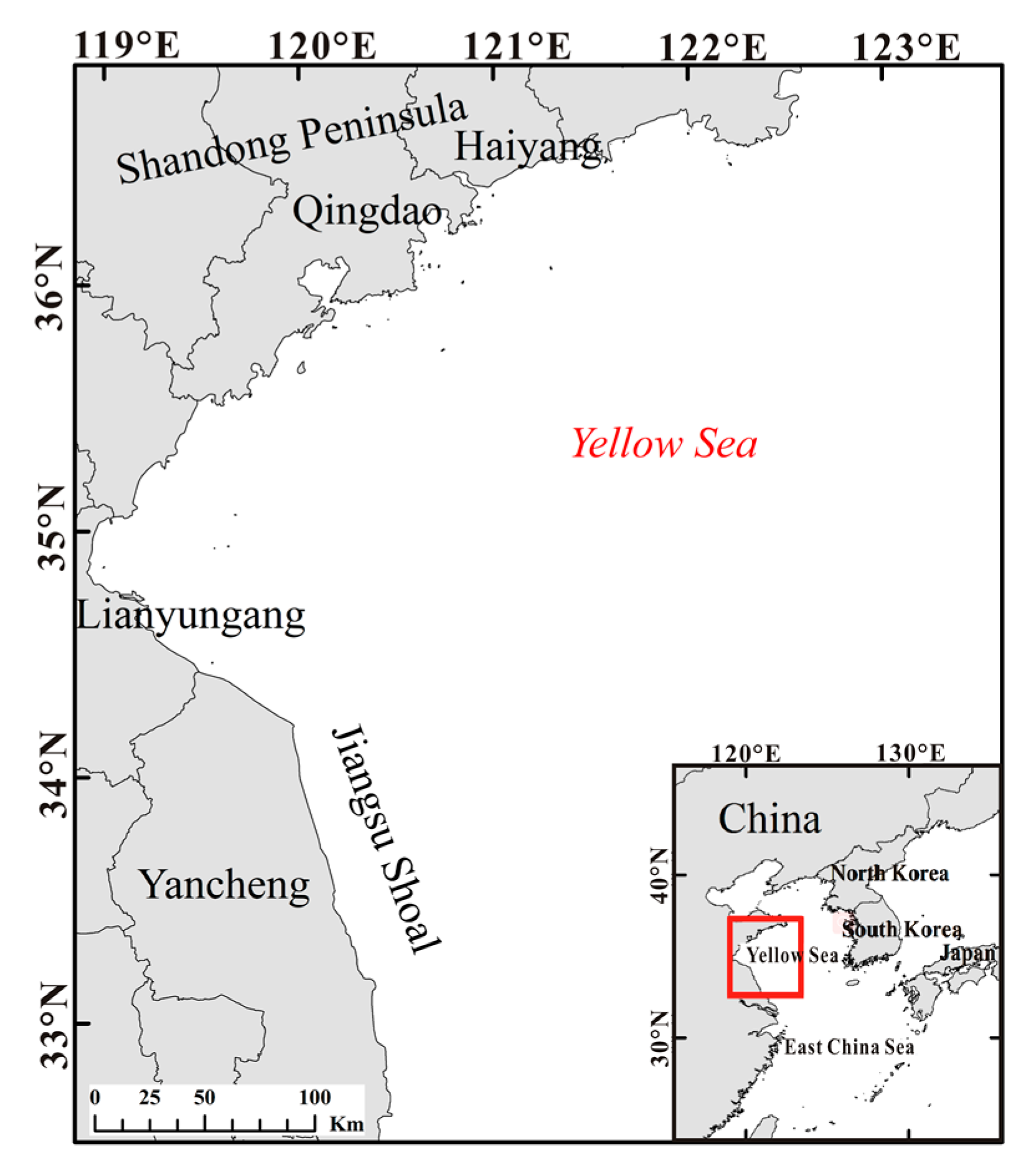
This study area belongs to the Southern Yellow Sea (119–123° E, 32–37° N), a part of the Yellow Sea in China. The Southern Yellow Sea is a semi-enclosed shallow sea with an average depth of 44 m (Figure 1) [31,32], covering an area of 309,000 km2. Influenced by the Yellow Sea Warm Current (YSWC), the Yellow Sea Cold Water Mass (YSCWM), the coastal current of the Yellow Sea, and the diluted current of the Yangtze River, the Southern Yellow Sea has complex hydrographic conditions [33]. In addition, the southern part of the study area is adjacent to the northern Jiangsu shoal, containing radial sand ridges. The special geographical location and climatic conditions make this area suitable for laver culture, and it has become the largest P. yezoensis culture base in China.
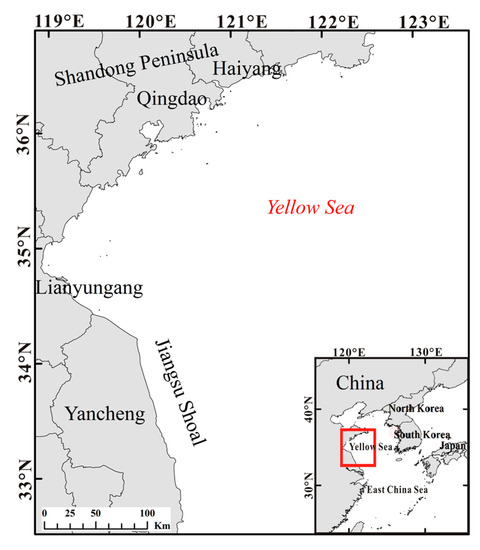
Figure 1.
Map of the study area in the Southern Yellow Sea, China.
2.2. Remote Sensing Data and Processing
Operations, such as remote sensing, data selection, and preprocessing, were completed on the GEE. In this paper, the remote sensing image data were used included atmospherically corrected surface reflectance data from the Landsat8 OLI/TIRS sensors and Level-2A orthorectified atmospherically corrected surface reflectance data from Sentinel-2/MSI sensors. Landsat8/OLI images have a revisit period of 16 days and a spatial resolution of 30 m, with 11 bands, of which the eighth is a panchromatic band. The spatial resolution of Sentinel-2/MSI imagery is 10 m, 20 m, and 60 m, with 13 bands, and the revisit period is five days. The parameters of the satellite images selected in this paper are shown in Table 1. The reason for choosing these data was that, compared with high temporal resolution satellite data (such as MODIS and GOCI), the high spatial resolution satellite images were more in line with the actual situation. This reduces the effect of mixed pixels on the extraction of algae (especially in the period of early growth) and improves the accuracy of disaster monitoring.

Table 1.
Satellite image information.
Among them, the satellite images of the same date were crop and mosaic so as to transform the multi-scene small image into a large range of one scene image. The land mask was a mask operation performed after importing China’s coastline data into GEE from 2016 to 2019. For the Landsat8/OLI images selected in this paper, the “Landsat. simpleCloudScore” cloud recognition and mask algorithm that comes with GEE was used. This algorithm added a “cloud” band to the image, with a band value of 0–100. The larger the value, the greater the possibility of clouds, so this paper set the value of the “cloud” band to 20. For the Sentinel-2/MSI images in the selected study area, this study used the QA60 band, which contains cloud information for cloud mask and image quality problems caused by cirrus clouds [34].
2.3. Field Data
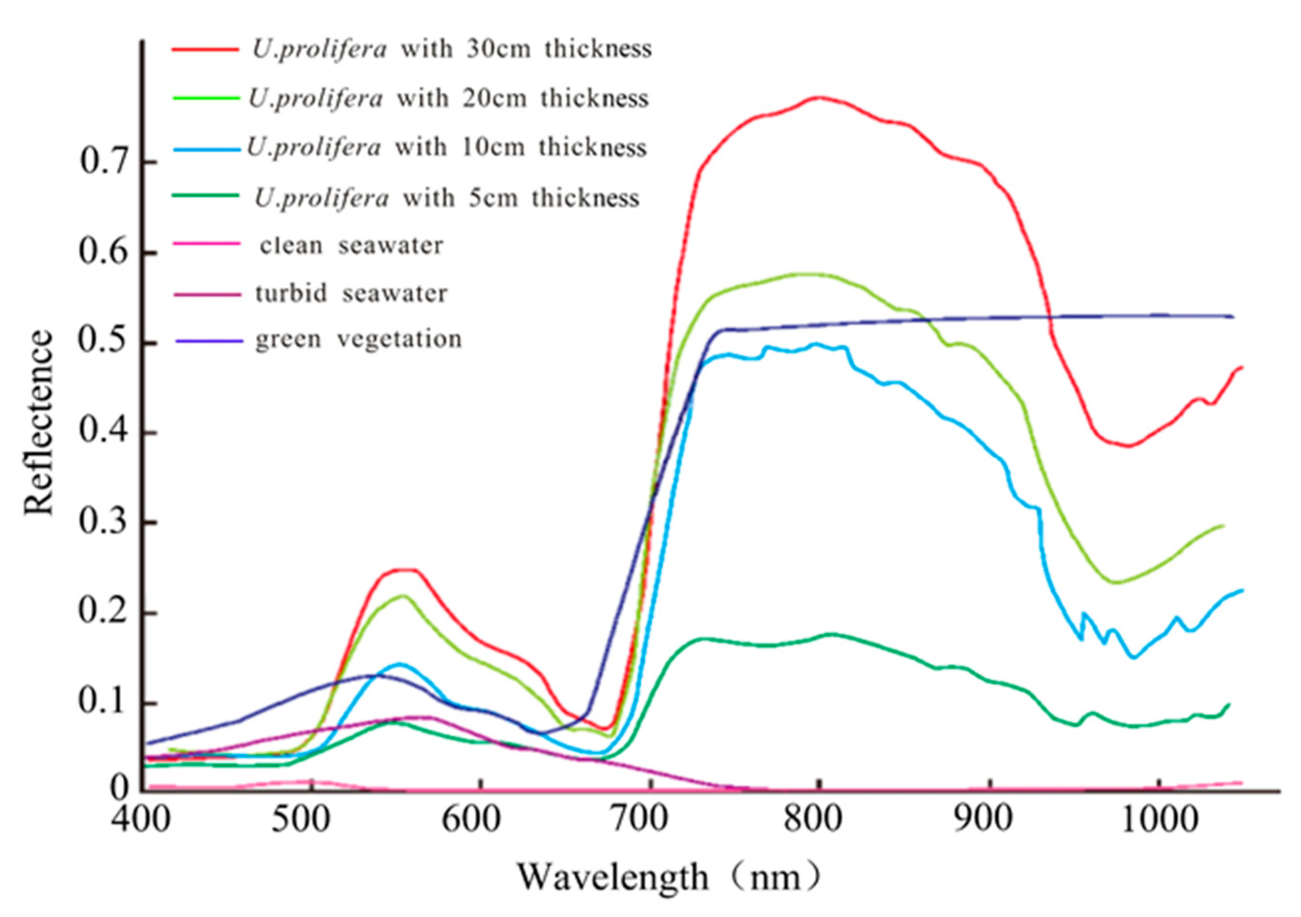
Unlike the traditional method of verifying satellite accuracy based on the field measurement data, it is very difficult to directly validate the U. prolifera detection from satellite data using field measurements. This is because the macroalgae are in a wide range and patchy, and it is difficult to obtain near-timely field measurements of the wide distribution. Therefore, the field data were collected mainly to understand the spectral characteristics of the algae in order to help the identification of it in seawater (Figure 2). In situ reflectance of living floating macroalgae was measured on 30 June 2017 and 04 July 2019 when green tides arrived in coastal waters off Haiyang. A fiber-optic probe with a 10° field of view connecting to a portable spectroradiometer (ASD FieldSpec) was pointed vertically 1 m over the sea surface to record the radiance of macroalgae (La, DN), and then pointed to a reference plaque with a calibrated reflectance of 0.25 to record the radiance of the plaque (Lp, DN); this procedure was repeated five times for every set of measurements to determine the mean La and Lp. Reflectance of algae was calculated as R (unitless) = La × 0.25/Lp [18].
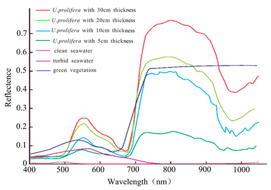
Figure 2.
Reflectance spectra of the U. prolifera and seawater measured in situ.
2.4. Methods
2.4.1. Normalized Difference Vegetation Index
In the past few years, the Normalized Difference Vegetation Index (NDVI) has been widely used in the extraction and classification of algae [35,36,37]. The calculation formula of NDVI is as follows:
where RNIR and RRED represent the reflectance of the near-infrared and infrared bands, respectively, in the atmospheric window. In the visible and near-infrared bands, U. prolifera showed similar spectral characteristics to green vegetation, and the reflectance curve of algae increased sharply near 700 nm (“red edge”). The reflectance of seawater in this band is low, so it is easy to distinguish U. prolifera floating in seawater. Generally, the NDVI value is between −1 and 1, the NDVI value of the water body is less than 0, and the NDVI value of U. prolifera is greater than 0. However, the NDVI value in each scene image was not constant due to weather conditions. Therefore, it was not reasonable to set the NDVI threshold as 0 to distinguish the algae from the water body. In specific cases, it was necessary to set the threshold based on a large number of threshold experiments and manual visual interpretation results. The fifth and fourth bands of the Landsat8/OLI image and the eighth and fourth bands of Sentinel-2/MSI imagery were selected to calculate NDVI in this study.
2.4.2. Floating Algae Index
In GEE, Landsat8/OLI and Sentinel-2/MSI atmospheric correction data were converted to Rayleigh-corrected reflectance (Rrc) by the following formula:
where is the calibrated sensor radiance after adjustment for ozone and other gaseous absorption, is the extraterrestrial solar irradiance at data acquisition time, is the solar zenith angle, and is Rayleigh reflectance [38].
NDVI values fluctuate greatly and are sensitive to environmental changes, such as aerosol type and thickness, solar angle and observation geometry, and sun glint [39,40]. Unlike the green vegetation growing on the land, the seawater strongly absorbs the light in the short-wave infrared band, so the seawater appears “black” in this band, forming a strong contrast with U. prolifera floating on the sea [18,41]. Based on this, Hu et al. proposed a baseline subtraction algorithm, which can correct the atmosphere simply and effectively [23]. FAI is calculated as follows:
where RRED, RNIR, and RSWIR represent the Rayleigh-corrected reflectance of the red, near-infrared, and short-wave infrared bands, respectively. , and represent the central wavelength of the red, near-infrared, and short-wave infrared bands, respectively. represents the baseline reflectance of the near-infrared band obtained by linear interpolation between the red band and the short-wave infrared band. Compared with the NDVI algorithm, the FAI value has a smaller fluctuation range. However, the FAI algorithm separated floating algae from other nonbloom sea waters very well. This is understandable because at the bloom–nonbloom boundary, there should be a sharp change (large gradient) in the FAI values [42]. The FAI algorithm was initially applied to MODIS images. The central wavelengths of the red, near-infrared, and short-wave infrared bands of MODIS images were 645 nm, 859 nm, and 1240 nm. There are many bands of Landsat8/OLI and Sentinel-2/MSI data. In this paper, the sixth, fifth, and fourth bands of Landsat8/OLI images (central wavelengths were 1610 nm, 865 nm, and 655 nm, respectively) and the tenth, fifth, and fourth bands of Sentinel-2/MSI imagery (central wavelengths were 1375 nm, 705 nm, and 665 nm, respectively) were selected for FAI calculation in this paper [43,44,45].
2.4.3. Canny Edge Filter and Otsu Thresholding
As mentioned above, the index was calculated from the spectral characteristics of algae. However, due to the influence of the environment, sensors, and other factors, the spectral properties of algae were different, which made the calculated values of algae index different. Therefore, it was necessary to intervene in the threshold selection algorithm manually. The Otsu thresholding algorithm is the most widely used. It is used to automatically find the best threshold through the image histogram obtained by least squares [46,47,48]. In the Otsu algorithm, the optimal threshold was based on maximizing the interclass variance (equivalently, it minimizes the sum of intraclass variances), as in Equation (4):
where BSS represents the between-sum-of-squares, describing the variance structure of a dataset; p is the number of classes, which in this study was 2. V is the value of the band selected to divide different classes. Class k is defined by every V less than a certain threshold. The optimal threshold is obtained by maximizing the BSS [49].
The Canny Edge Filter was originally used to extract the boundary between rivers and the land. Here, the Canny Edge Filter was applied to the boundary between algae and seawater to improve the extraction accuracy of micro-U. prolifera scattered in the sea [50]. It should be noted that the distribution of the histogram appeared at the junction of the seawater and U. prolifera pixels. Therefore, the filter was buffered, and a buffer area of 10 m × 10 m was established at the edge [51]. In this paper, the parameters (sigma and threshold) of the Canny Edge Filter were set to = 0.1, = 0.01. The and parameters were used to define the standard deviation of the Gaussian smoothing kernel and the sensitivity of the filter, respectively.
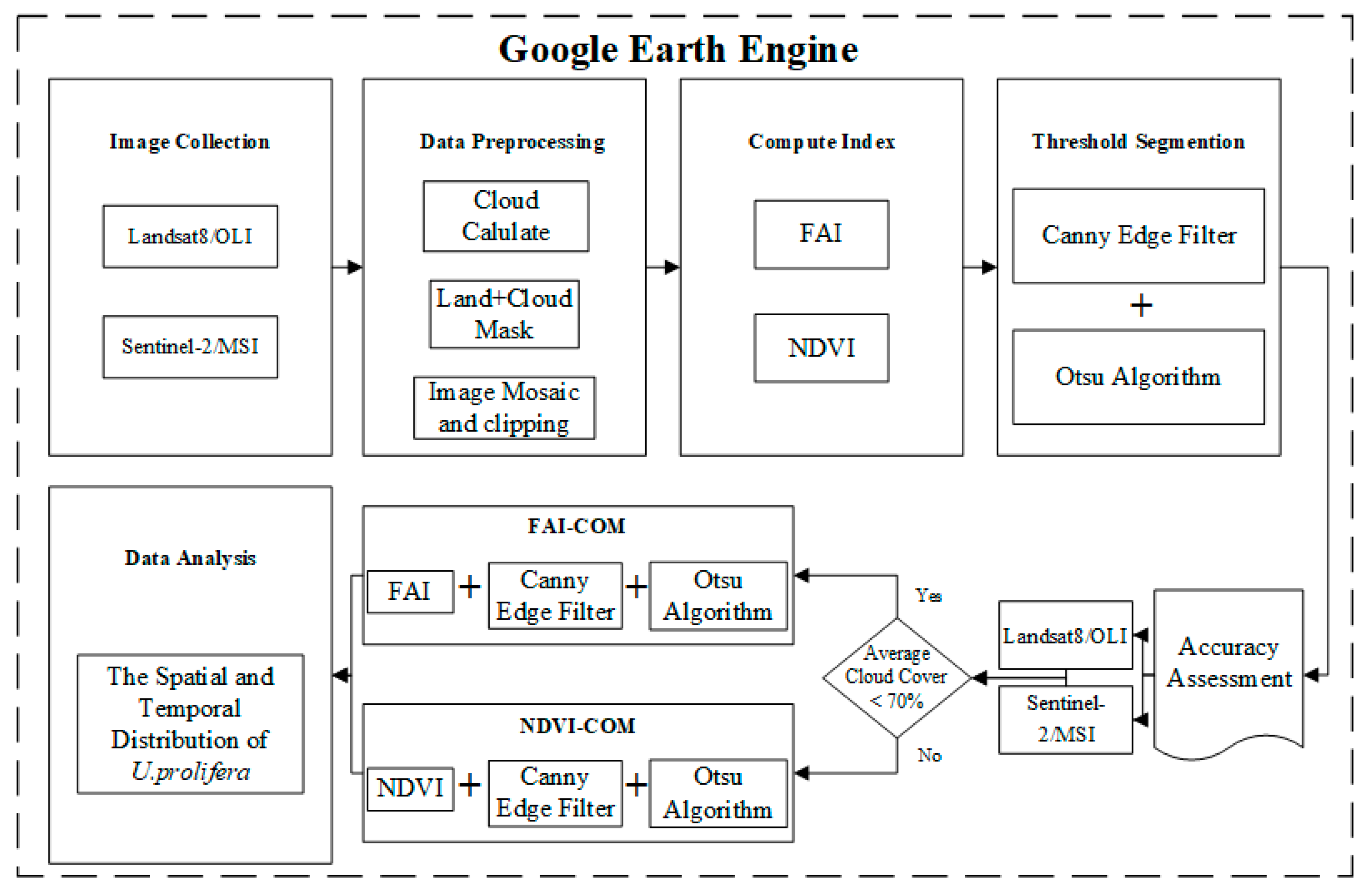
2.4.4. Model Building
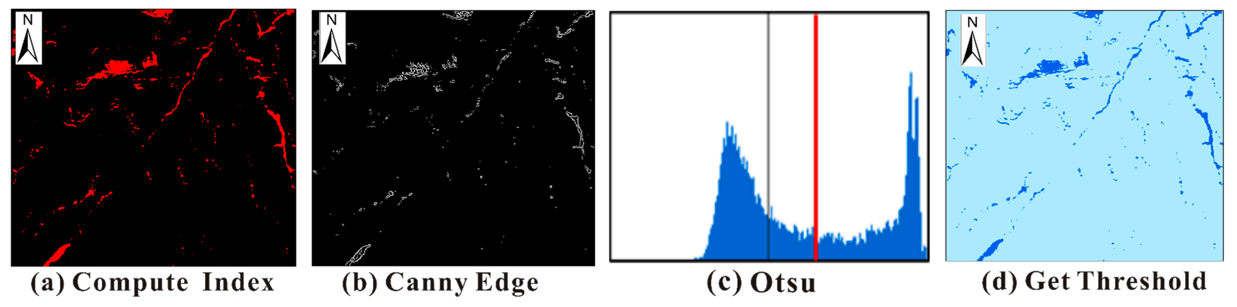
In this paper, the adaptive threshold detection model, which enables fast and automated threshold selection by adding the Otsu threshold algorithm of the Canny Edge Filter based on algal calculation indices (FAI, NDVI), was used. It should be noted that this model only achieved a threshold when there was algae occurred in the seawater (we first perform FAI or NDVI calculation on the image before performing Canny Edge Filter and Otsu segmentation). When the model used the FAI algorithm, it was named FAI-COM (model based on FAI, the Canny Edge Filter, and Otsu thresholding). When the model used the NDVI algorithm, it was named NDVI-COM (model based on NDVI, the Canny Edge Filter, and Otsu thresholding). A demonstration of each module in the model is shown in Figure 3 (the gray line in Figure 3c represents the threshold only based on Index, and the red line represents the optimal threshold line based on Canny Edge Filter and Otsu method).

Figure 3.
Demonstration of each algorithm in GEE.
The model was embedded into the GEE platform. After preprocessing the image data, the threshold values in different areas could be automatically selected, which greatly improved the efficiency of monitoring U. prolifera based on remote sensing methods. The technical route of this paper is shown in Figure 4. It should be noted that, after assessing the accuracy of the model, this paper determined the condition for using FAI-COM or NDVI-COM to generate U. prolifera results, and the condition was whether “the average cloud cover was <70% (for all images on the same date in the study area)”. See Section 3.1 and Section 4.1 for details.
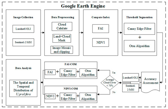
Figure 4.
Workflow of adaptive threshold detection model.
3. Results
3.1. Model Accuracy and Applicability
3.1.1. Ground Truth
In this paper, we took the visual interpretation of macroalgae on the image as the ground truth for the model verification because the green macroalgae floating on the water surface has a generally similar spectral property to land vegetation in the visible and NIR wavelengths with a typical red-edge signal (700 nm). Moreover, based on previous research results, macroalgae disasters are often a single species in the study area. Although other algae, such as Sargassum, may be found in some years, the spectral reflectance characteristics of these algae are significantly different [52]. Therefore, the pixels of algae could be determined by comparing the spectral reflectance characteristics of satellite images (Figure 5) and in situ measured U. prolifera (Figure 2). In essence, visually determined algae slicks can be used as the ground truth [24].
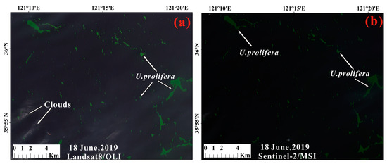
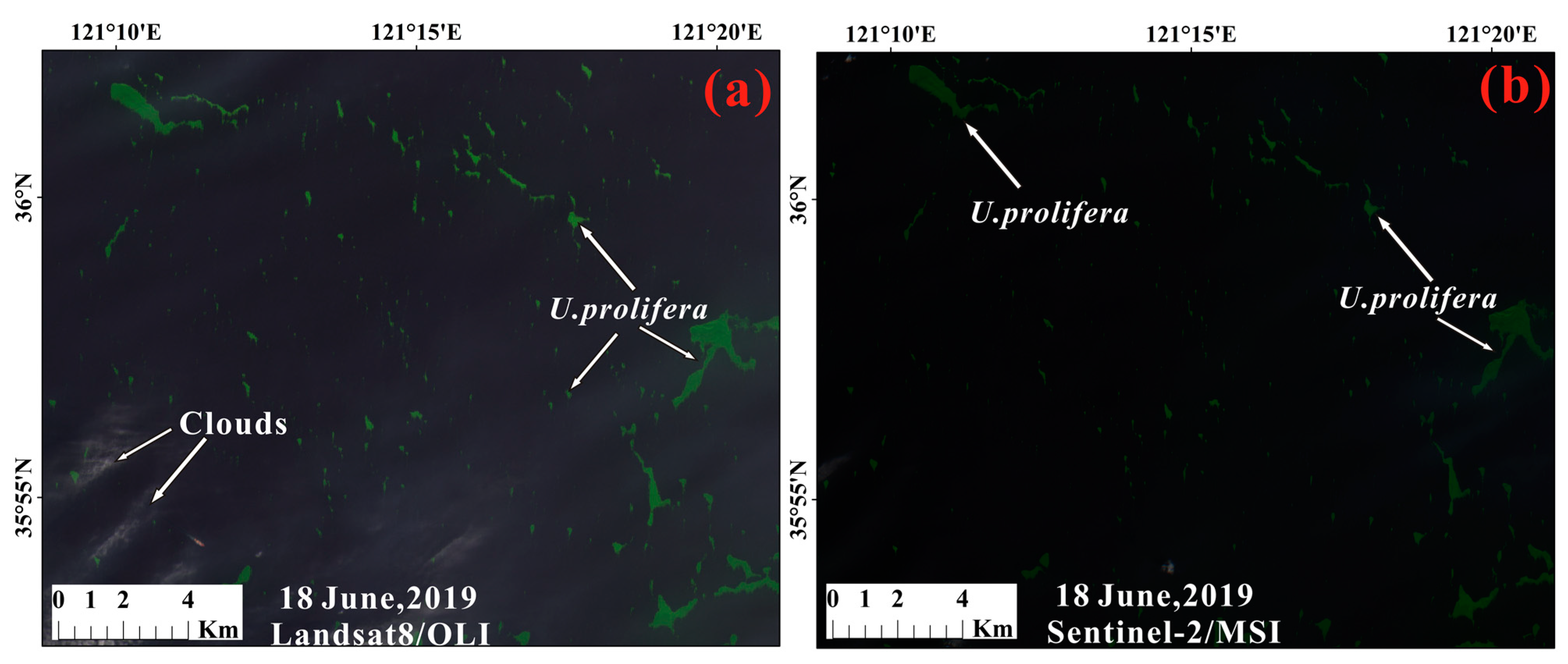
Figure 5.
A visual interpretation of the satellite Red-Green-Blue “true-color” composite image recorded by Landsat8/OLI and Sentinel-2/MSI. (a) Landsat8/OLI true-color image on 18 June 2019, R:G:B = band 4:3:2, (b) Sentinel-2/MSI true-color image on 18 June 2019, R:G:B = band 4:3:2.
3.1.2. Accuracy Comparison Based on Cross-Sensor
Influenced by the environment and physiological characteristics, the spectral reflectance of U. prolifera is different in different periods [12,15,53]. In this study, we selected some images of U. prolifera at different scales and dates to verify the accuracy of the model. Compared with Landsat8/OLI image, Sentinel-2/MSI data have a short revisit period and high resolution (10 m). The method of artificial visual interpretation can be used to verify the accuracy of the model with Sentinel-2/MSI data.
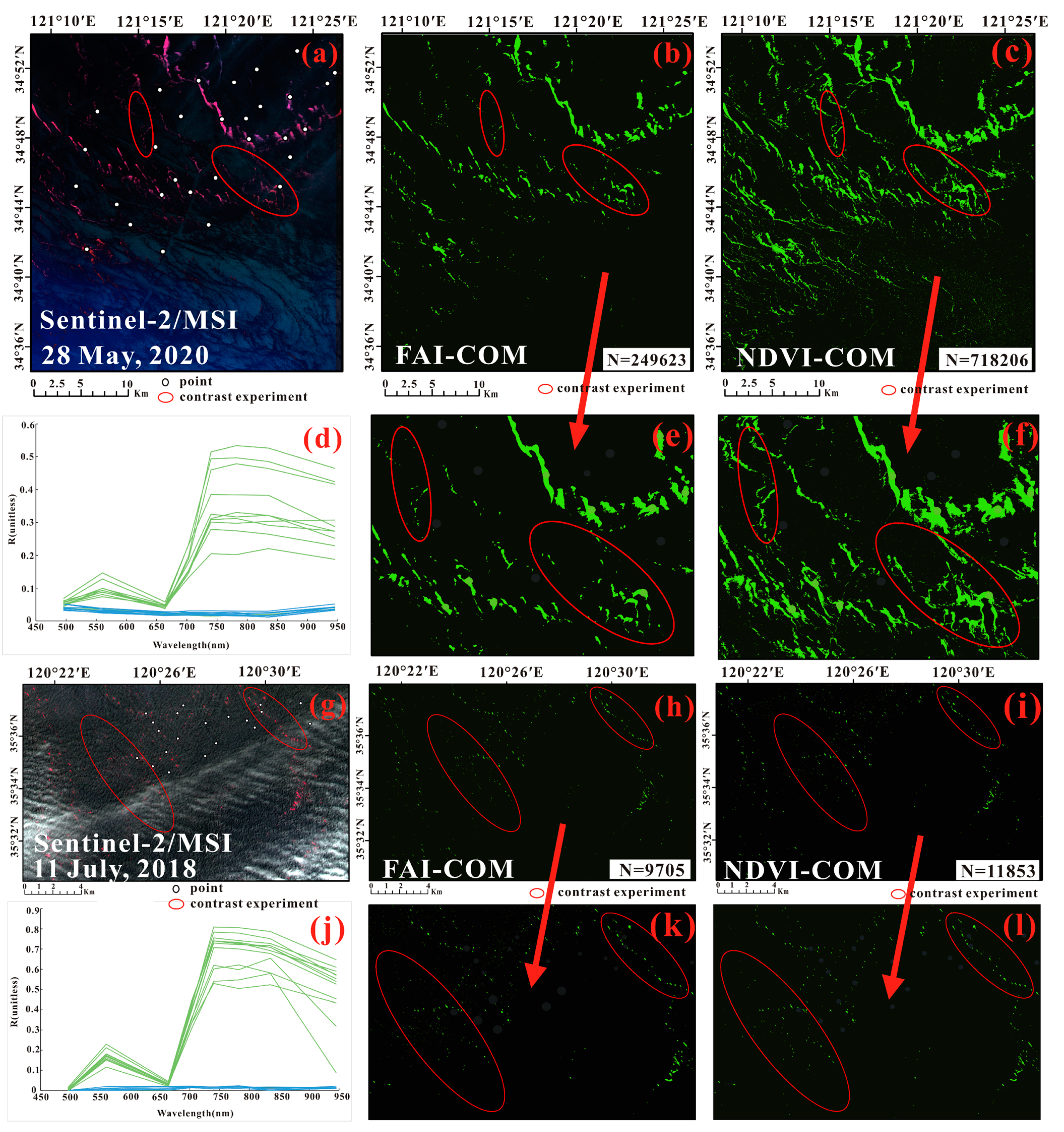
On 3 June 2018, U. prolifera appeared red in the Sentinel-2/MSI false-color image. Then, combined with the spectral characteristics of random sampling points in Figure 6d, we found U. prolifera was mainly distributed in the sea area near the P. yezoensis culture area in the northern Jiangsu shoal and appeared sporadically at a small scale. The FAI-COM and NDVI-COM were calculated, and a comparison map of U. prolifera extraction was obtained, as shown in Figure 6b,c. As shown in the red circles, the U. prolifera prevalence extracted based on FAI-COM was more consistent with the distribution of U. prolifera in the image, while there were more algae pixels extracted by NDVI-COM (N = 207,164, “N” means the number of U. prolifera pixels) than by FAI-COM (N = 199,731), which was inconsistent with the actual situation.
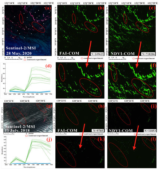
Figure 6.
Comparison of U. prolifera extraction from Sentinel-2/MSI images on 28 May 2020 (a–f) and 11 July 2018 (g–l). “N” means the number of U. prolifera pixels. (a,g) Sentinel-2/MSI pseudo-true-color image, R:G:B = band 8:4:3, (b,h) U. prolifera extracted from FAI-COM, (c,i) U. prolifera extracted from NDVI-COM, (d) reflectance spectra with random points of U. prolifera and seawater corresponding to the eight Sentinel-2 bands on 28 May 2020, (e,f) enlarged view of (b,c), respectively, (j) reflectance spectra with random points of U. prolifera and seawater corresponding to the eight Sentinel-2 bands on 11 July 2018, (k,l) enlarged view of (h,i), respectively.
On 11 July 2018, according to the spectral characteristics of random sampling points and visual interpretation of macroalgae in Figure 6, it was found that the U. prolifera were scarce and distributed sporadically in the south of Qingdao City, Shandong Province. FAI-COM and NDVI-COM were calculated for this image. As shown in Figure 6g, there were a few thin clouds. However, U. prolifera were distributed under thin clouds. In the red circles, the extracted distribution of algae based on FAI-COM (N = 9705) was more consistent with the distribution of U. prolifera in this image, and the number of U. prolifera pixels was less than that extracted by NDVI-COM (N = 11,853). The image of thin cloud pixel also had a higher NDVI value, which increased the extraction number of U. prolifera pixels.
Comparing the extraction of U. prolifera in the red circles of Figure 6, it can be found that the model based on the NDVI algorithm (NDVI-COM) was classified into pure pixels of U. prolifera by mistake under the same parameters, which led to the overall number of U. prolifera pixels being more than that of FAI-COM. This phenomenon exists in remote sensing images of U. prolifera at different scales and dates. Due to the influence of satellite image quality, atmospheric environment conditions (thin clouds, sun glint), and satellite resolution, NDVI-COM is affected by environmental changes and has poor robustness. Therefore, the model based on the FAI algorithm (FAI-COM) is more suitable for extracting U. prolifera from the Sentinel-2/MSI image.
As mentioned above, this paper takes the Sentinel-2/MSI image data with higher spatial resolution as the true values and uses them to perform a cross-sensor comparison on Landsat8/OLI image data of relatively low resolution. From 2016 to 2020, there were four scenes of Landsat8/OLI and Sentinel-2/MSI images with the same date in the study area, as shown in Table 2.
Table 2.
Landsat8/OLI and Sentinel-2/MSI image data.
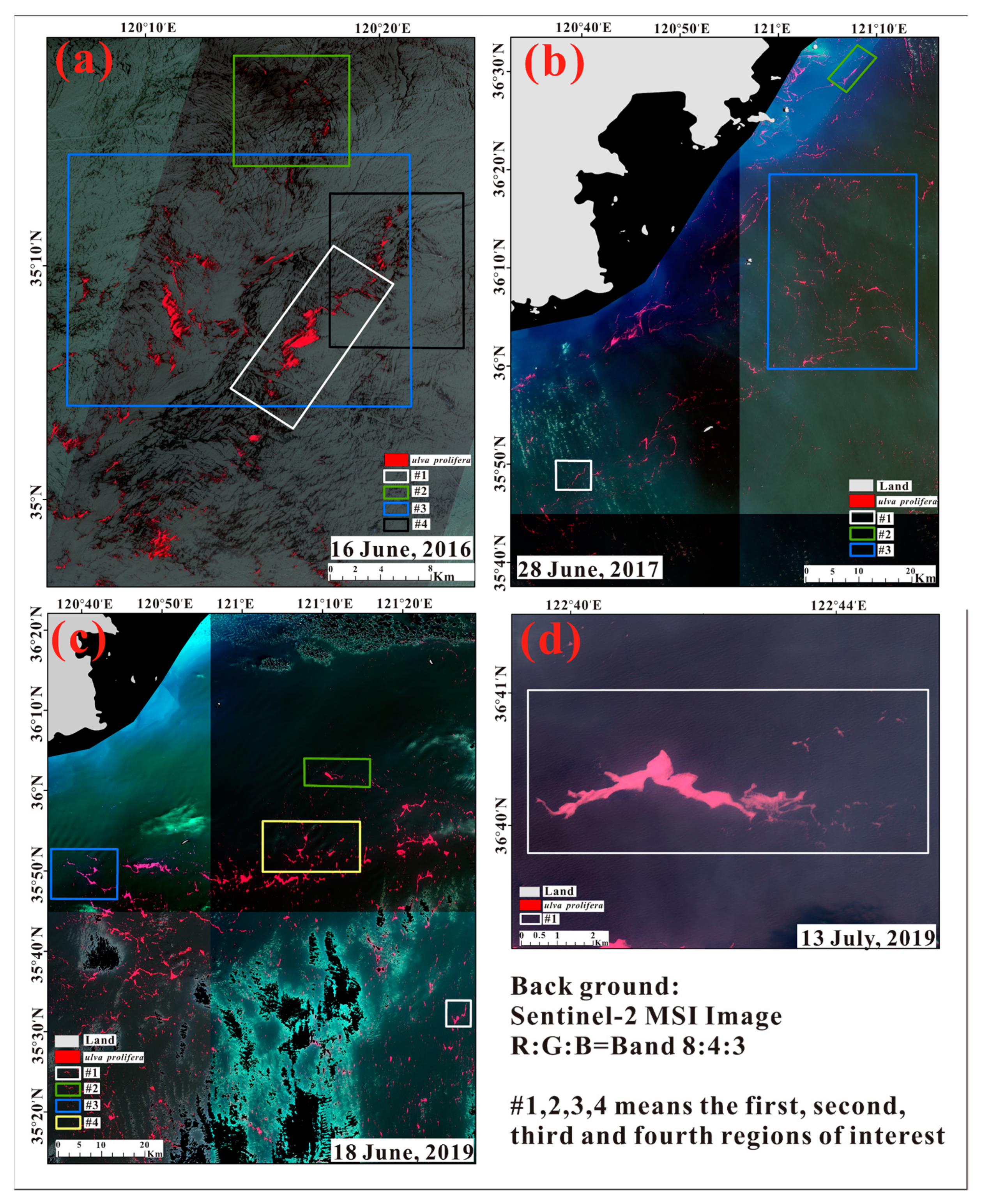
The width of the Landsat8/OLI image is unlike that of the Sentinel-2/MSI image. For better accuracy, different regions of interest were randomly selected from the overlapping regions of two kinds of images. The distribution of regions of interest (ROI) is shown in Figure 7. It should be noted that on 13 July 2019, there were a large number of clouds in the study area, and there were few U. prolifera in the Landsat8/OLI images on that day, so only one region of interest was selected.
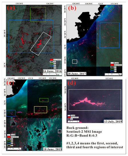
Figure 7.
Map of regions of interest. (a) Distribution map of four ROI on 16 June 2016, (b) Distribution map of three ROI on 28 June 2017, (c) Distribution map of four ROI on 18 June 2019, (d) A distribution map of one ROI on 13 July 2019.
Next, the above data were processed. As shown in Figure 8, the extraction comparison map of interest area was obtained by the model (FAI-COM and NDVI-COM).
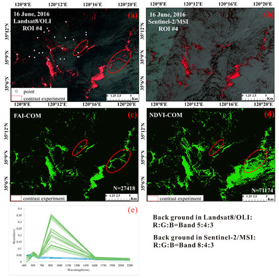
Figure 8.
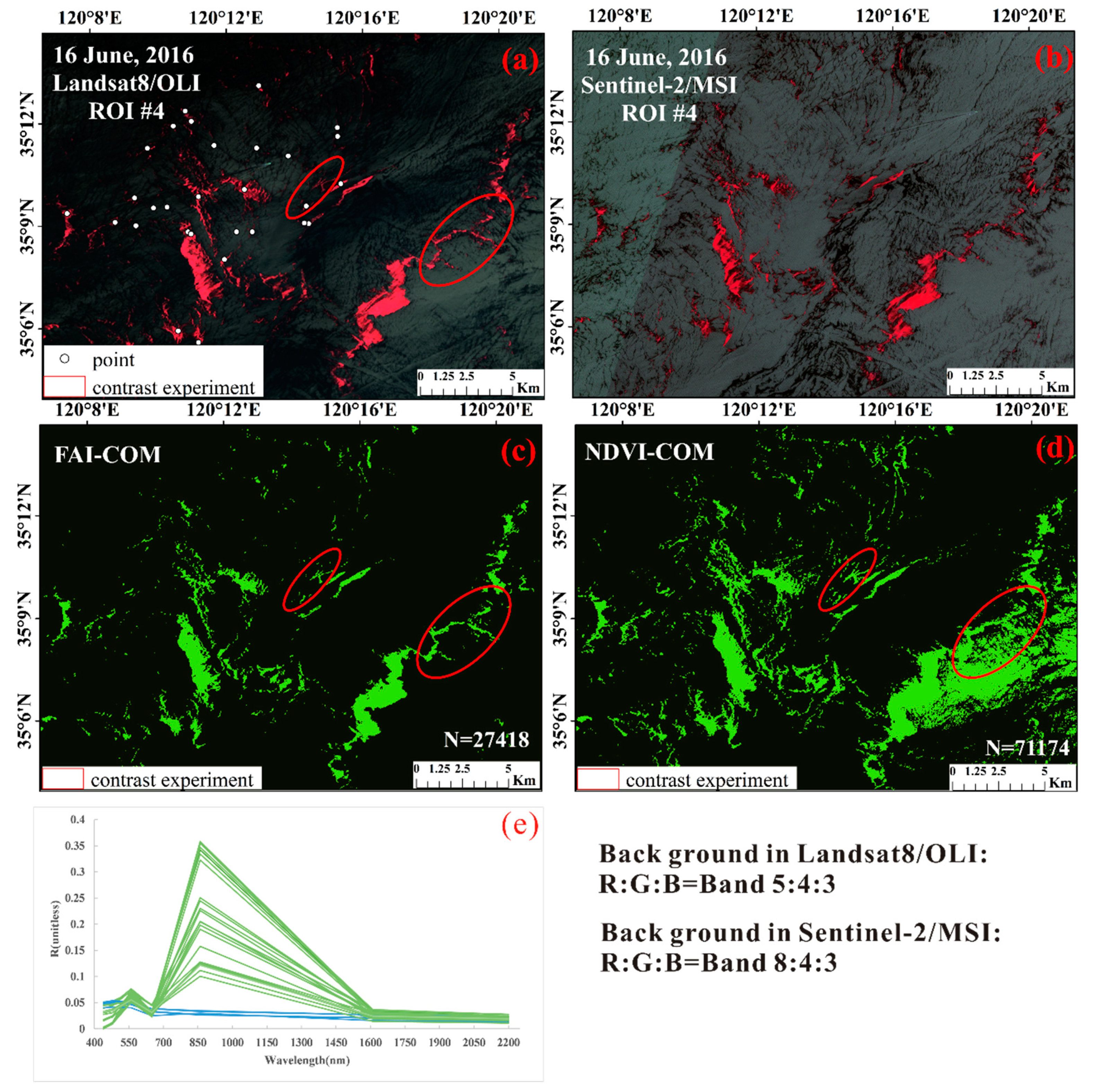
Comparison of U. prolifera extraction in #4 ROI on 16 June 2016. “N” means the number of U. prolifera pixels. (a) Landsat8/OLI pseudo-true-color image, R:G:B = band 5:4:3, (b) Sentinel-2/MSI pseudo-true-color image, R:G:B = band 8:4:3, (c) U. prolifera extracted from FAI-COM, (d) U. prolifera extracted from NDVI-COM, (e) reflectance spectra with random points of U. prolifera and seawater corresponding to the seven Landsat8 bands on 16 June 2016.
Figure 8 reveals that, similar to the Sentinel-2/MSI imagery on the same date, the Landsat8/OLI imagery on 16 June 2016 also had sun glint. The distribution of U. prolifera from FAI-COM (N = 27,418) was closer to the distribution of the U. prolifera in the actual image. The distribution of U. prolifera extracted by NDVI-COM (N = 71,174) was misclassified in the pixels because of the sun glint, which made the overall classification of U. prolifera pixels increase and not conform to the actual situation. This phenomenon was similar to the misclassification of U. prolifera in Sentinel-2/MSI images (Figure 6a).
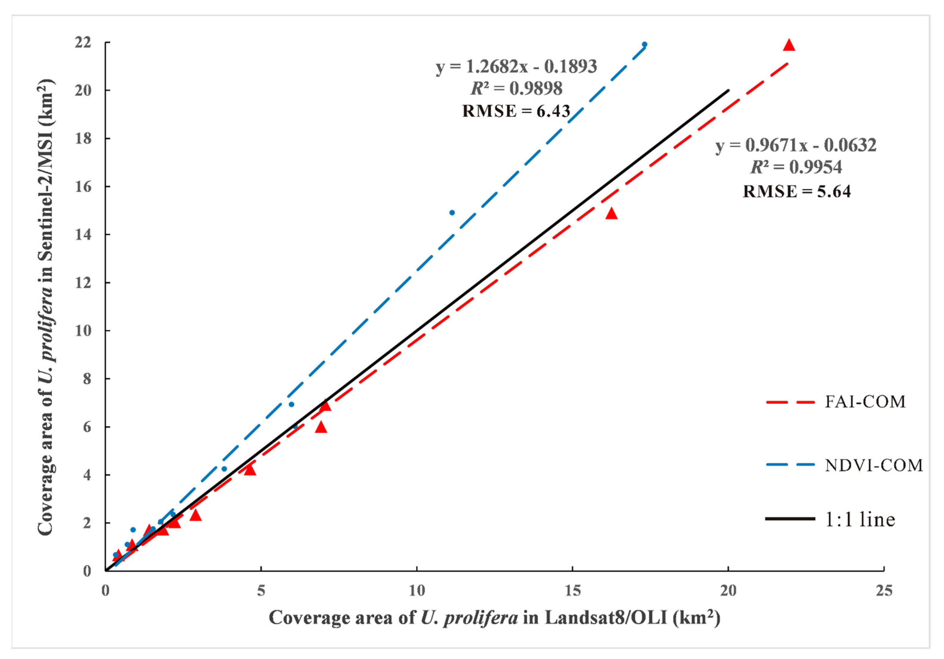
This paper analyzed the correlation between the area of U. prolifera extracted from the two algorithm models (Figure 9). The correlation results showed that, through study area thresholds, the area of U. prolifera extracted by two models were well correlated (greater than 0.9), but the root mean square error of FAI-COM was small (RMSE = 5.64).

Figure 9.
Accuracy comparison of two models for extracting U. prolifera in Landsat8/OLI images. The coverage area of U. prolifera in Sentinel-2/MSI is taken as the true value.
Overall, the accuracy of FAI-COM was higher in Landsat8/OLI and Sentinel-2/MSI images, but when there were more clouds (such as 13 July 2019) in the imagery, FAI-COM was no longer applicable. Therefore, the average cloud cover of the image was calculated in the study area from 2016 to 2020, and then the cloud cover information of the date was counted when FAI-COM was not applicable to extract algae (Table 3).
Table 3.
Statistical table of cloud cover information in the date when FAI-COM was not able to extract U. prolifera.
Based on the statistical results of the average cloud cover of images in Table 3, the condition of using FAI-COM or NDVI-COM was set to 70% of the average cloud cover of all images on the same date. Then, the FAI-COM was used to generate U. prolifera results in the study area when the average cloud cover was less than 70% (model parameter: = 0.1, = 0.01); on the contrary, NDVI-COM was used to generate U. prolifera results when the average cloud cover more than 70% (model parameter: = 0.1, = 0.1). See Section 4.1.1 for detailed analysis.
3.1.3. Accuracy Comparison Based on Confusion Matrix
A total of 15 Sentinel-2/MSI images from 2016 to 2020 were selected as training samples, as well as for evaluation of the confusion matrix of the two models (FAI-COM and NDVI-COM) used in Landsat8/OLI images. A confusion matrix is a common method for evaluating the accuracy of two or more classes of classification and is often used to evaluate the performance of classification methods. Based on the confusion matrix, the overall accuracy (OA), user accuracy (User acc.), F1 score, and Kappa coefficients were calculated [54,55,56]. The classification of 15 test images was determined by the algorithm index and visual interpretation experience. These independent images with a representative environment (clear sky, thin clouds) and aggregate conditions were used as training samples. The statistical table of the confusion matrix of the model is shown in Table 4, where the overall classification accuracy of the model was above 0.9 with a high kappa coefficient value. The F1 score of the U. prolifera in the confusion matrix was above 0.8 overall. These results showed that the F1 score of the U. prolifera was lower than 0.8 on 12 June 2017, 19 June, and 22 June 2018, and 27 June, 1 July, and 13 July 2019. On these days, there were a lot of clouds in the Landsat8/OLI images (Table 3), and only a small amount of U. prolifera was distributed at the edge of the cloud. In these circumstances, NDVI-COM was able to classify U. prolifera. In addition, the resolution of Landsat8/OLI images was lower than the Sentinel-2/MSI sample data, and NDVI-COM classified more mixed pixels of algae, which led to the lower F1 scores of the model.
Table 4.
Confusion matrix of FAI-COM and NDVI-COM.
We applied this model to Landsat8/OLI and Sentinel-2/MSI images and then performed U. prolifera extraction. The F1 score of U. prolifera extracted by the combined model was above 0.85. The results showed that the model had high extraction accuracy and strong robustness to environmental changes, as well as better applicability.
3.2. Spatio-Temporal Distribution of U. prolifera
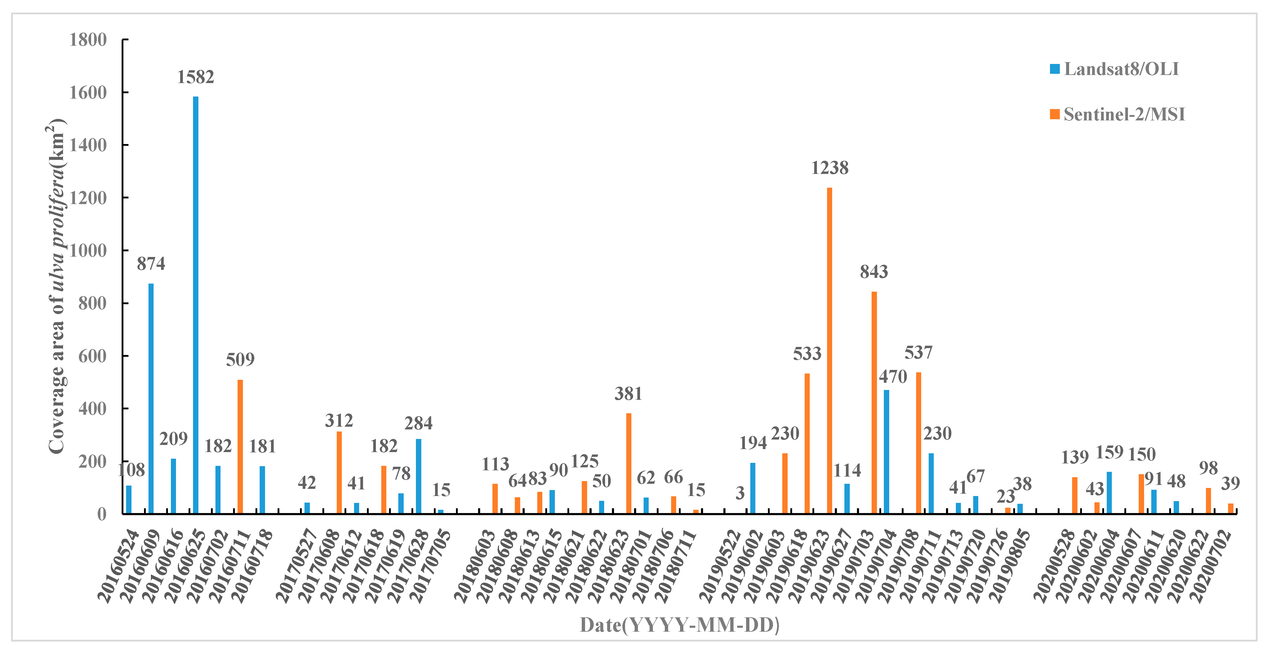
Based on the adaptive threshold calculated by the model, the coverage area and spatiotemporal distribution of U. prolifera in the study area over five years were generated from Landsat8/OLI and Sentinel-2/MSI images (Figure 10 and Figure 11).

Figure 10.
Statistical chart of U. prolifera area based on Landsat8/OLI and Sentinel-2/MSI satellites in the study area from 2016 to 2020.
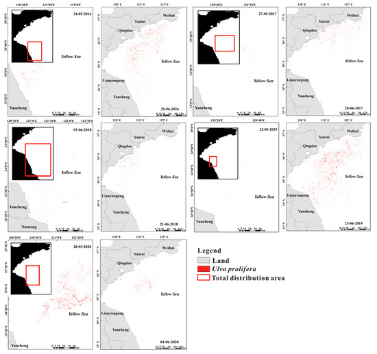
Figure 11.
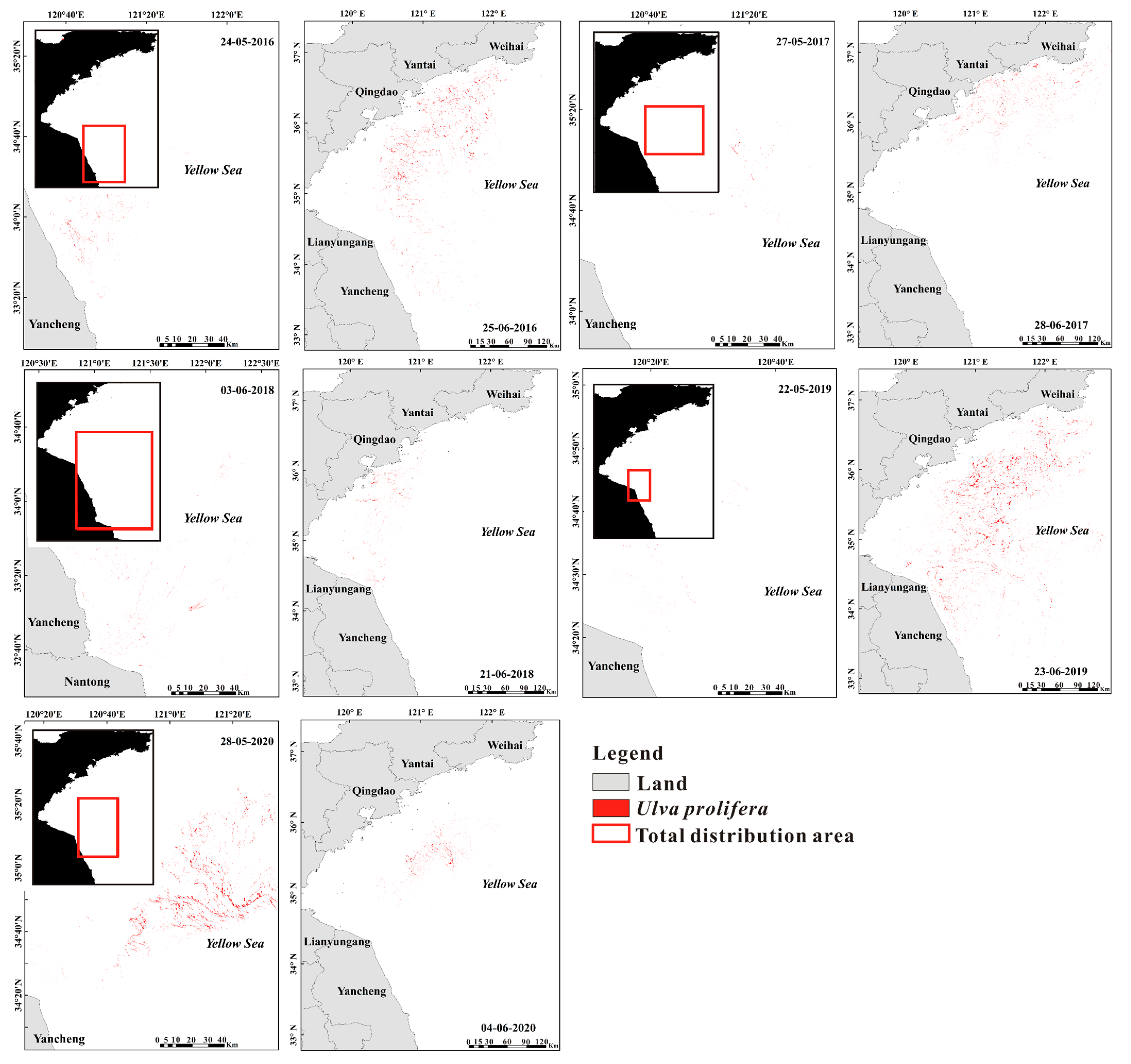
Temporal and spatial distribution of U. prolifera in the study area from 2016 to 2020. Only two representative images with the earliest discovery date and the largest daily area of U. prolifera were selected for each year.
On 25 June 2016, U. prolifera had the largest scale and the widest distribution range (from the eastern sea area of Yancheng City, Jiangsu Province to the southern sea area of Weihai City, Shandong Province). The daily coverage area of U. prolifera was about 1582 km2, which was the largest coverage area of U. prolifera in the five years. In general, 2016 was the largest outbreak of U. prolifera in the five years. Previous studies have shown that 2015 was the most serious year of the U. prolifera disaster in the study area. After that, in 2016, the coverage area of U. prolifera decreased, but the distribution scope and duration persisted [57,58,59].
Compared with 2016, the daily coverage area of U. prolifera in 2017 showed a significant downward trend. On 28 June 2017, U. prolifera had the largest scale, mainly distributed in the sea area near the Shandong Peninsula (Qingdao City, Yantai City, and Weihai City), with a daily coverage area of about 284 km2. In 2016, the first discovery date of U. prolifera was 24 May; it covered an area of 108.07 km2 in the northeast sea area of Yancheng City, Jiangsu Province. In 2017, the first discovery date of U. prolifera was 27 May; it covered an area of 39.59 km2, and the sea area where U. prolifera gathered was also near Yancheng City, Jiangsu Province. The largest area was on 28 June in that year, with a daily coverage of about 284 km2. U. prolifera was mainly distributed in the sea area near Yantai City with Sentinel-2/MSI data. There was no rebound in the outbreak scale of U. prolifera in 2018. Sentinel-2/MSI images showed that on 21 June 2018, U. prolifera had the largest scale, and was mostly distributed in the southern sea area of Qingdao City, and a small part was in the sea area near Yancheng City. The daily coverage area of U. prolifera was about 125 km2. In 2018, U. prolifera was first found on 3 June (Sentinel-2/MSI image). At this time, U. prolifera was distributed in the eastern sea area of Yancheng City, Jiangsu Province, with daily coverage of about 113 km2. Affected by the weather conditions in 2018 and 2020, Landsat8/OLI images only monitored the distribution of U. prolifera in June. The outbreak scale in these two years was much smaller than that in 2016.
In 2019, the outbreak scale of U. prolifera increased compared to the previous three years. On 23 June, U. prolifera broke out at the largest scale. Through Sentinel-2/MSI images, it was shown that algae were distributed in most of the sea areas of Shandong Peninsula and Yancheng City, Jiangsu Province, with a daily coverage of about 1238 km2. The outbreak scale in 2019 was like that in 2016. On 22 May, a Sentinel-2/MSI pseudo-true-color image showed U. prolifera floating in the sea area near the northeast of Yancheng City. After that, algae were detected again on 2 June, when the coverage area was about 194 km2.
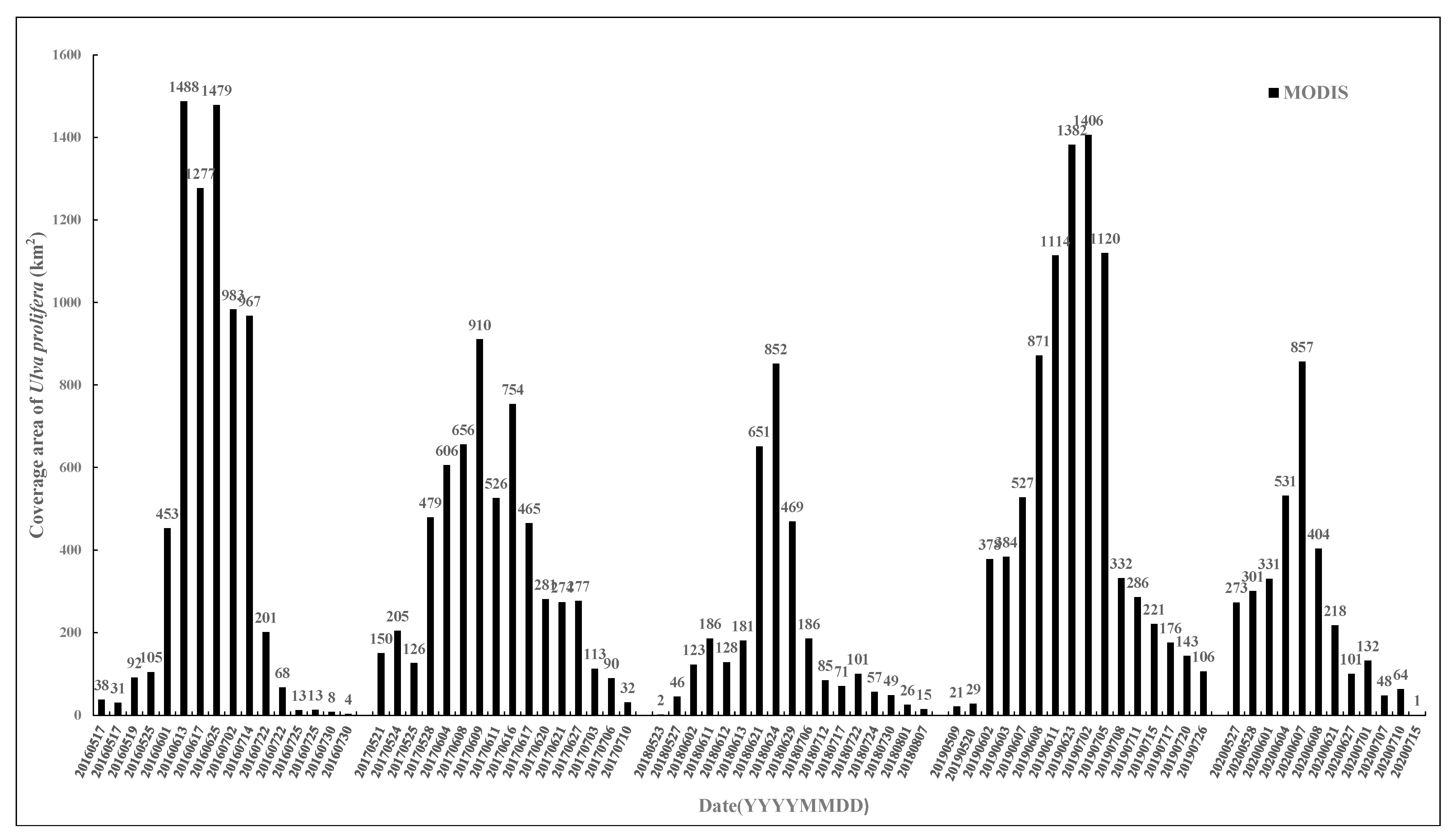
It should be noted that the Landsat8/OLI and Sentinel-2/MSI data cannot cover the whole study area. Therefore, in order to reflect the trend of the distribution area of U. prolifera more accurately over the past five years, MODIS data were selected in this paper. Then preprocessed MODIS Level-1A images, such as radiation correction, atmospheric correction, and geometric correction, were extracted from the distribution area of U. prolifera by artificial visual interpretation. The MODIS results (Figure 12) were similar to the scale of U. prolifera reported by the Ministry of Natural Resources North China Sea Administration.
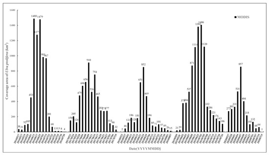
Figure 12.
Statistical chart of U. prolifera area based on MODIS satellite in the study area from 2016 to 2020.
Through the annual average statistics of the coverage area of U. prolifera in the five years (Figure 13), it was found that the area showed a decreasing trend year by year. And the results of MODIS were consistent with those of Landsat8/OLI and Sentinel-2/MSI. In general, the interannual coverage of U. prolifera in 2017, 2018, and 2020 was relatively small, while that of 2016 and 2019 was relatively large. Among the Landsat8/OLI and Sentinel-2/MSI results, the annual average area of algae in 2016 was the largest (521 km2); compared with 2017 and 2018, the annual mean coverage of algae in 2019 increased to about 326 km2.
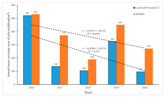
Figure 13.
Statistical chart of annual mean coverage area of U. prolifera.
Compared to Figure 10, the daily coverage area of U. prolifera in Figure 12 was larger, which was related to the existence of many mixed pixels in MODIS images (many pixels may be mixed with both water and macroalgae). It was also related to the smaller width of Landsat8/OLI and Sentinel-2/MSI satellites, which did not cover the whole area. But the area of U. prolifera in the early stage (late May to early June) over the five years in Figure 12 was similar to that in Figure 10. By contrast, high-resolution satellite images were more suitable for the extraction of the early stage of the algae because the coverage area of U. prolifera was small and scattered in patches in this stage. In addition, the largest daily coverage area extracted by the model in this paper was similar to the data of the China Marine Disasters Bulletin from 2008 to 2019. Overall, the combined results of Landsat8/OLI and Sentinel-2/MSI can support the monitoring and early warning of U. prolifera in the study area.
4. Discussion
4.1. Evaluation of the Model
4.1.1. Advantages of the Model
(1) The advantage of the adaptive threshold extraction model is that it can select the threshold automatically for the whole research area. The model integrates the advantages of the FAI algorithm and has high stability. That is, when the dynamic threshold calculated from a large area was applied to the extraction of U. prolifera in a small area, the extraction result was similar to the actual distribution area of U. prolifera.
Therefore, this paper selected four Landsat8/OLI images with repeated dates in Section 3.1, used the thresholds obtained in the whole study area to calculate the extraction area of U. prolifera in the ROI (small area), and then compared the stability of the model (Figure 14). It should be noted that the dynamic threshold model could extract the threshold in different ranges and had high accuracy (as shown in Figure 9). Therefore, the true value in Figure 14 was the area of U. prolifera, extracted by the dynamic threshold model based on the ROI in Sentinel-2/MSI images.
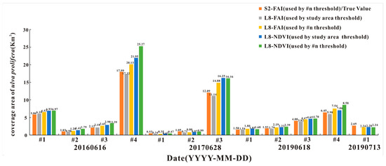
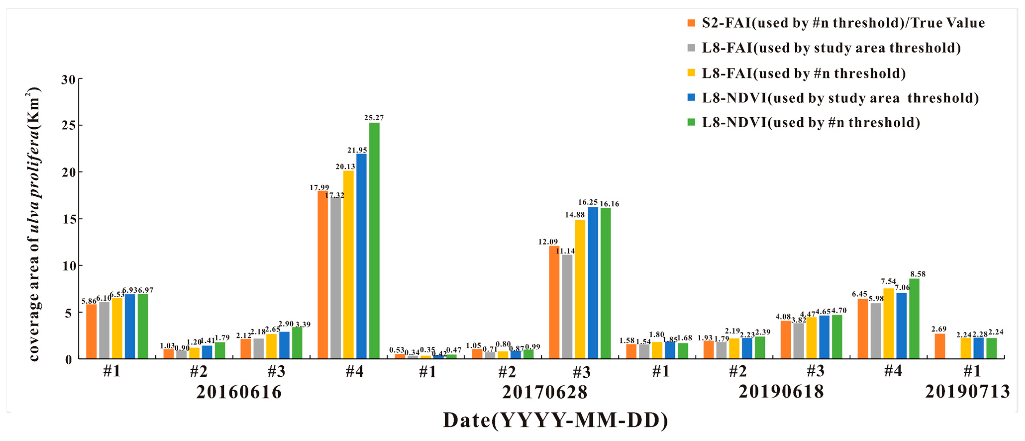
Figure 14.
Statistical map of U. prolifera area. “S2” represents Sentinel-2/MSI images, “L8” represents Landsat8/OLI images, “used by #n threshold” represents the area of U. prolifera based on the threshold of the n-th ROI, n = 1, 2, 3, 4, “used by study area threshold” represents the area of U. prolifera based on the threshold of the whole study area.
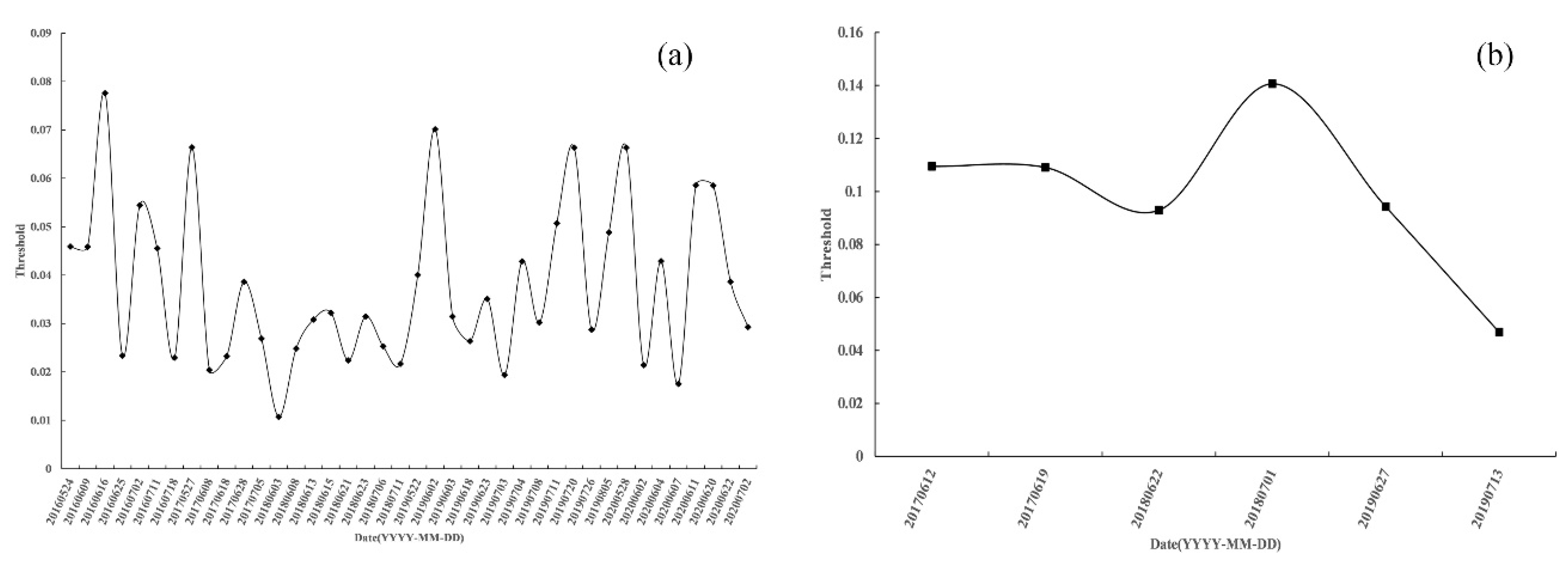
It can be seen from Figure 14 that, based on NDVI-COM, under the threshold of the whole study area, the extracted area of U. prolifera was larger than that of the Sentinel-2/MSI image on the same date. Based on FAI-COM, the area of U. prolifera from the whole study area was similar to the true area of U. prolifera, and the area change was small. Therefore, the adaptive threshold model based on FAI is more stable and accurate. This is mainly because the value fluctuation range of FAI is small (Figure 15), which makes the area of U. prolifera extracted between different thresholds change less.

Figure 15.
Statistical of optimal threshold of U. prolifera in the study area from 2016 to 2020: (a) threshold by FAI-COM; (b) threshold by NDVI-COM.
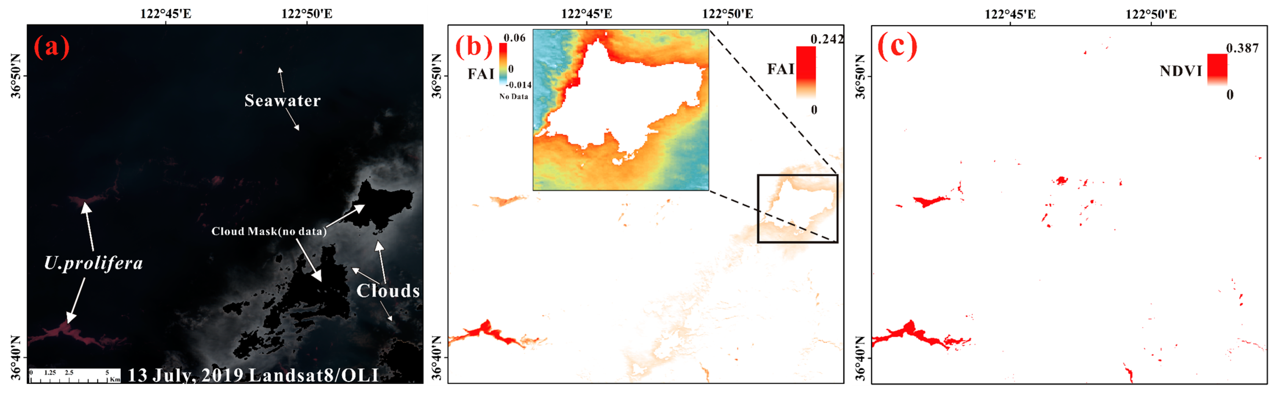
(2) By adjusting the parameters of the Canny Edge Filter ( = 0.1), the NDVI-COM realized the adaptive threshold extraction of U. prolifera when the average cloud cover was more than 70%. This is because, in the NDVI algorithm, the values of cloud and seawater were generally negative [60,61]. The parameter of the Canny Edge Filter can determine the minimum gradient magnitude, and the sigma parameter () is the standard deviation (SD) of a Gaussian prefilter to remove high-frequency noise. When was set to a larger value (such as 0.1, the minimum gradient magnitude was similar to the difference in NDVI value between cloud and algae), the model could extract algae at the edge of thick clouds.
As mentioned above, the average cloud cover of Langsat8/OLI image on 13 July 2019 was higher than 70%. As shown in Figure 16, the cloud mask algorithm provided by GEE could not mask the cloud well, and a small part of algae was distributed at the edge of the cloud. After calculating the FAI and NDVI of the image, we found that the remaining cloud had a high FAI value (the maximum is about 0.06), while the NDVI value was negative. The higher FAI value of cloud could affect the threshold selection of the model, which made the FAI-COM no longer applicable at this time.

Figure 16.
Schematic diagram of the model. (a) Landsat8/OLI pseudo-true-color image on 13 July 2019, R:G:B = band 5:4:3, (b) the result of FAI value greater than 0 on 13 July 2019, and the black box is the result of FAI value in cloud area, (c) the result of NDVI value greater than 0 on 13 July 2019.
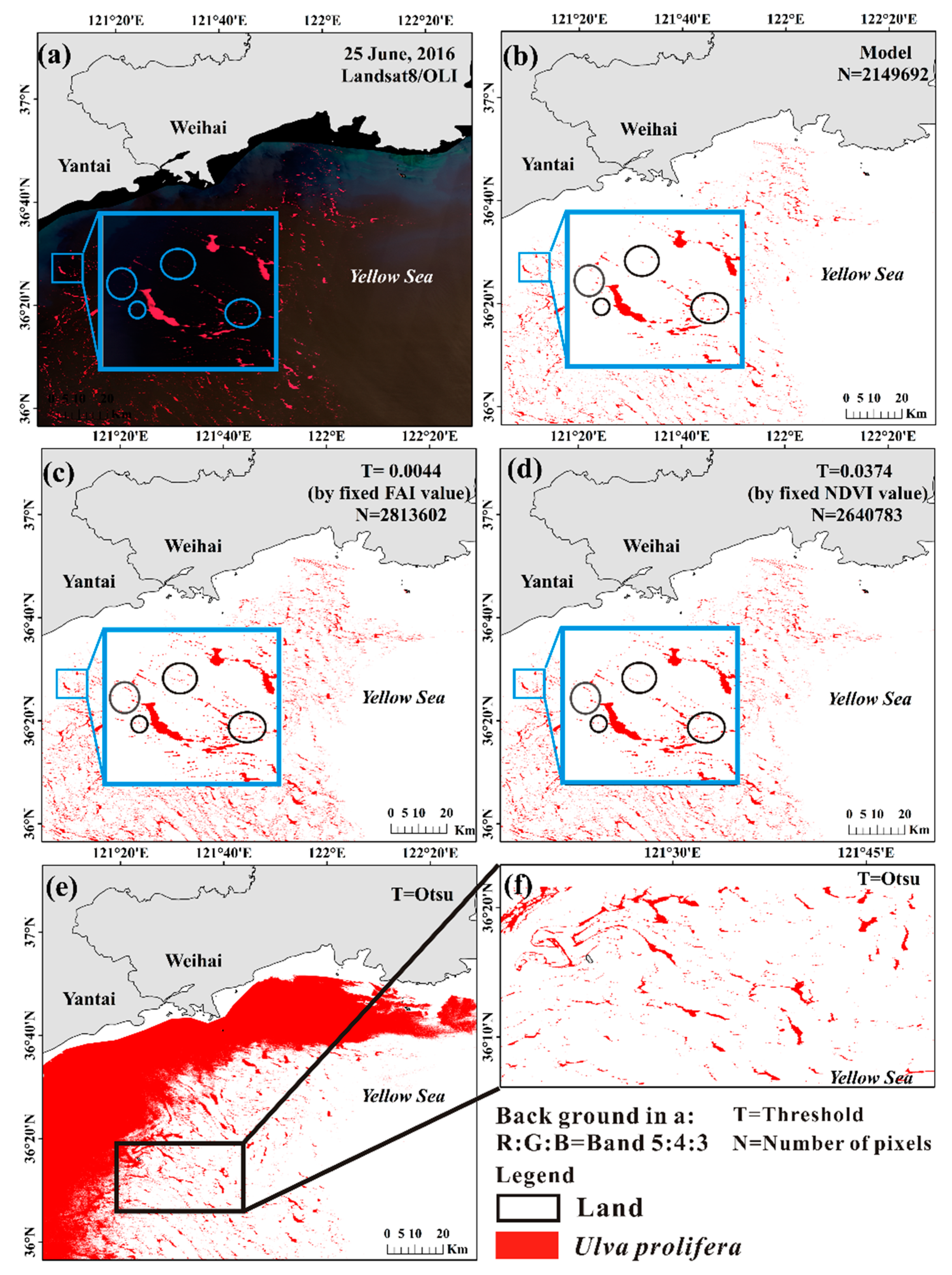
(3) Another advantage of the dynamic threshold is that, compared with the fixed threshold, the extracted area of U. prolifera was more in line with the actual situation. Using the threshold extraction method by Hu et al. [42], this paper first calculated the mean and standard deviation by all individual images. Then, the fixed threshold was obtained by the mean minus two standard deviations. As shown in Figure 17b–d, in the sea area near Yantai City, Shandong Province on 25 June 2016, the fixed FAI threshold (T = 0.0044, Mean threshold value = 0.0378, and Stdev threshold value = 0.0167) and the fixed NDVI threshold (T = 0.0374, Mean threshold value = 0.0988, and Stdev threshold value = 0.0307) were not suitable for the extraction of U. prolifera while the dynamic threshold model in this paper could accurately extract U. prolifera. We found that the number of algae pixels extracted by the fixed threshold method (NFAI = 2813602 and NNDVI = 2640783) were more than the model proposed in this paper (NModel = 2149692), and it was not consistent with the distribution of U. prolifera in Figure 17a.
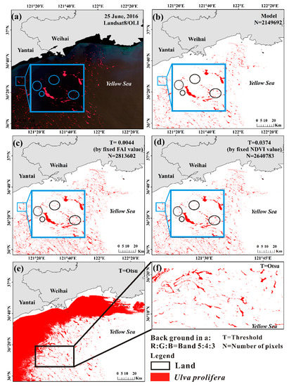
Figure 17.
Comparison of adaptive threshold model with other methods. The blue box is the zoom of the same area in (a–d). (a) Landsat8/OLI pseudo-true-color image on 25 June 2016, R:G:B = band 5:4:3, (b) distribution map of U. prolifera based on the model in this paper, (c) distribution map of U. prolifera based on a fixed FAI threshold of 0.0044, (d) distribution map of U. prolifera based on a fixed NDVI threshold of 0.0374, (e) distribution map of U. prolifera based on the Otsu method, (f) distribution map of U. prolifera based on the Otsu method from the black box area in (e).
The Otsu threshold algorithm had defects in extracting U. prolifera on 25 June 2016, as shown in Figure 17e,f. The results showed that the Otsu algorithm was not suitable for large-scale threshold selection because the number of seawater pixels was far more than that of U. prolifera. When the research area was reduced, the Otsu algorithm showed better threshold selection results (Figure 17f). Compared with the Otsu algorithm, the dynamic threshold model in this paper was more suitable for a wide study area of threshold selection, which was related to the Canny Edge Filter added to the model. This filter improved the defects of the Otsu algorithm so that it only classified the edge pixels of U. prolifera and seawater by a histogram, limiting the area of the Otsu algorithm [62].
4.1.2. Uncertainty of the Model
(1) The construction of the model was mainly based on the GEE. The advantage of the GEE lies in its fast and convenient cloud processing operation, which saves a lot of time for remote sensing image preprocessing. However, the remote sensing image data provided in GEE are limited, such as HJ-1A/B CCD, Gaofen, and VIIRS (Visible Infrared Imager/Radiometer Suite); other remote sensing image data are not used, so the applicability of the model to cross-sensor image data needs to be studied further. However, the band combination required by the NDVI is suitable for most satellite images, while the short-wave infrared band required by the FAI is not suitable for some satellite images. This problem can be solved by adding the VB-FAH algorithm [18] into the model so as to achieve fast and dynamic extraction of U. prolifera through multi-sensors.
(2) When there are more clouds in the image, the accuracy of the model will be affected. Although this situation can be avoided by choosing an image with a cloud cover less than 20%, the fact that U. prolifera distribution in the image with cloud cover of more than 20% is ignored. The cloud mask algorithm provided by GEE is not effective and will misclassify algae pixels into cloud pixels. Due to the failure of the FAI-COM, using NDVI-COM is a compromise method.
4.2. The Critical Period for the Growth and Spread of U. Prolifera
The growth of U. prolifera is inseparable from the suitable temperature and rich nutrients. As it happens, the special geographical conditions of Jiangsu shoal and the Porphyra culture environment provide support for the growth of U. prolifera. During the period from the end of May to the beginning of June, the early stage of U. prolifera was detected by remote sensing data, floating in the sea area near Jiangsu shoal, and the daily coverage increased day by day. Therefore, this period can be inferred as a critical period for the growth and spread of U. prolifera [63].
Figure 10 shows that the distribution of U. prolifera was originally discovered at the end of May in 2016 and 2019, covering areas of 108 km2 and 3 km2, respectively. The distribution of U. prolifera in early June of 2018, 2019, and 2020 was roughly similar, covering areas of 113 km2, 194 km2, and 159 km2, respectively. The coverage of U. prolifera in early June of 2016 and 2017 was relatively high at 874 km2 and 312 km2, respectively. Overall, from the end of May to the beginning of June, a higher coverage area of U. prolifera distribution was observed during the five years. However, compared with 2016 and 2019, the overall scale of U. prolifera in 2017 and 2018 showed a decreasing trend (Figure 10). Wang found that, in 2017 and 2018, in the waters near Sheyang City, Jiangsu Province, early floating U. prolifera were salvaged and cleaned up. Therefore, the overall coverage of U. prolifera in these two years was relatively small [64].
Previous studies have shown that the growth rate of U. prolifera attached to the raft in April and May is not higher than 12.5% per day. When U. prolifera falls off the raft, the growth rate of U. prolifera floating on the sea will reach 20% per day [65]. The number of U. prolifera attached to the raft is very small, and difficult to detect by remote sensing satellite. Through UAV and field observation, Xing et al. learned that, in 2016, P. yezoensis facilities were recycled in mid-May [65]. While the recycling in 2017 and 2018 was at the end of May, the biomass of U. prolifera was 46% and 18% in the other two years of the same period; follow-up studies showed that P. yezoensis facilities were recycled in early May in 2019, and the biomass of U. prolifera was higher in May. This delayed the recycling time of P. yezoensis facilities, and thus the delay in the shedding of attached algae into seawater may be the reason for the short time and low amount of U. prolifera growth and spread in 2017 and 2018. In summary, the early warning and monitoring of U. prolifera play a very important role. Early control and management of the source of U. prolifera (such as the recovery and cleaning of P. yezoensis culture facilities and the salvage of U. prolifera) can effectively curb the annual biomass.
5. Conclusions
Based on Google Earth Engine, this study used an adaptive threshold model to extract U. prolifera. The model was applied to Sentinel-2/MSI and Landsat8/OLI images to extract and analyze the distribution of U. prolifera in the South Yellow Sea, China from 2016 to 2020. The results show that:
- (1)
- The model first performed Floating Algae Index (FAI) or Normalized Difference Vegetation Index (NDVI) algorithms on the preprocessed remote sensing images and then used the Canny Edge Filter and Otsu threshold segmentation algorithm to automatically extract the threshold.
- (2)
- The model extraction of U. prolifera based on the FAI algorithm has higher accuracy (R2 = 0.99, RMSE = 5.64) and better robustness. However, when the average cloud cover is more than 70% in the image (based on the statistical results of multi-year cloud cover information), the model based on the NDVI algorithm has better applicability and can extract the algae distributed at the edge of the cloud. Therefore, the final extraction results were generated by supplementing NDVI-COM results on the basis of FAI-COM extraction results in this paper. Further, the F1-score of U. prolifera extracted by the combined model was above 0.85.
- (3)
- From 2016 to 2020, the interannual change in U. prolifera in the study area showed a decreasing trend. The overall outbreak scale of U. prolifera in 2017 and 2018 was relatively small, which was related to the delay in the recycle time of P. yezoensis culture facilities in the Northern Jiangsu shoal and the artificial salvage of U. prolifera in May. In contrast, early warning and cleanup measures were not taken in 2019, and the outbreak scale of U. prolifera rebounded.
Compared with the traditional threshold selection and the Otsu threshold algorithm, the model proposed in this paper is more convenient and accurate for the extraction of U. prolifera, and it has high robustness to environmental changes. This article focused on a case study in the South Yellow Sea, China, where green tides frequently occur. It is hoped that it can bring scientific and technical support to the monitoring and early warning of green tides in the study area.
Author Contributions
Conceptualization, G.Z., G.X.; methodology, G.Z.; software, H.L.; validation, G.Z., J.W.; formal analysis, L.N.; investigation, Y.H.; resources, G.Z.; data curation, G.Z.; writing—original draft preparation, G.Z.; writing—review and editing, M.W.; visualization, G.X.; supervision, G.X.; project administration, G.X.; funding acquisition, G.X. All authors have read and agreed to the published version of the manuscript.
Funding
This work is supported by the Shenzhen Science and Technology Program (Grant No. KQTD20180410161218820), the National Natural Science Foundation of China (No. 42071385), and the Shandong Natural Science Foundation (No. ZR2019MD041).
Institutional Review Board Statement
Not applicable.
Informed Consent Statement
Informed consent was obtained from all subjects involved in the study.
Data Availability Statement
The data presented in this study are available upon request from the corresponding author.
Acknowledgments
The remote sensing data of Google Earth Engine are available online at https://earthengine.google.com/ (accessed on 10 July 2021). Data of the U.prolifera by the Ministry of Natural Resources North China Sea Administration are available online at http://ncs.mnr.gov.cn/ (accessed on 10 July 2021). The statistical data of U.prolofera by the China Marine Disasters Bulletin from 2008 to 2019 are available online at http://www.mnr.gov.cn/ (accessed on 10 July 2021). In the end, the authors like to thank the anonymous reviewers for their efforts and constructive comments to improve the quality of this paper.
Conflicts of Interest
The authors declare no conflict of interest.
References
- Lapointe, B.E.; Burkholder, J.M.; van Alstyne, K.L. Harmful macroalgal blooms in a changing world: Causes, impacts, and management. In Harmful Algal Blooms: A Compendium Desk Reference; John Wiley: Hoboken, NJ, USA, 2018; pp. 515–560. [Google Scholar]
- Wang, M.; Hu, C. Mapping and quantifying Sargassum distribution and coverage in the Central West Atlantic using MODIS observations. Remote Sens. Environ. 2016, 183, 350–367. [Google Scholar] [CrossRef]
- Hu, C.; Cannizzaro, J.; Carder, K.L.; Muller-Karger, F.E.; Hardy, R. Remote detection of Trichodesmium blooms in optically complex coastal waters: Examples with MODIS full-spectral data. Remote Sens. Environ. 2010, 114, 2048–2058. [Google Scholar] [CrossRef]
- Hu, C.; He, M.X. Origin and offshore extent of floating algae in Olympic sailing area. Eos Trans. Am. Geophys. Union 2008, 89, 302–303. [Google Scholar] [CrossRef]
- Liu, D.; Keesing, J.K.; Xing, Q.; Shi, P. World’s largest macroalgal bloom caused by expansion of seaweed aquaculture in China. Mar. Pollut. Bull. 2009, 58, 888–895. [Google Scholar] [CrossRef]
- Xing, Q.; Hu, C.; Tang, D.; Tian, L.; Tang, S.; Wang, X.H.; Lou, M.; Gao, X. World’s largest macroalgal blooms altered phytoplankton biomass in summer in the Yellow Sea: Satellite observations. Remote Sens. 2015, 7, 12297–12313. [Google Scholar] [CrossRef] [Green Version]
- Peggy Fong, R.M.D.; Zedler, J.B. Competition with macroalgae and benthic cyanobacterial mats limits phytoplankton abundance in experimental microcosms. Mar. Ecol. Prog. Ser. 1993, 100, 97–102. [Google Scholar] [CrossRef]
- Wang, C.; Yu, R.-C.; Zhou, M.-J. Effects of the decomposing green macroalga Ulva (Enteromorpha) prolifera on the growth of four red-tide species. Harmful Algae 2012, 16, 12–19. [Google Scholar] [CrossRef]
- Zhang, X.; Luan, Q.-S.; Sun, J.-Q.; Wang, J. Influence of Enteromorpha prolifera (Chlorophyta) on the phytoplankton community structure. Mar. Sci. 2013, 37, 24–31. [Google Scholar]
- Liu, D.; Keesing, J.K.; Dong, Z.; Zhen, Y.; Di, B.; Shi, Y.; Fearns, P.; Shi, P. Recurrence of the world’s largest green-tide in 2009 in Yellow Sea, China: Porphyra yezoensis aquaculture rafts confirmed as nursery for macroalgal blooms. Mar. Pollut. Bull. 2010, 60, 1423–1432. [Google Scholar] [CrossRef]
- Liu, D.; Keesing, J.K.; He, P.; Wang, Z.; Shi, Y.; Wang, Y. The world’s largest macroalgal bloom in the Yellow Sea, China: Formation and implications. Estuar. Coast. Shelf Sci. 2013, 129, 2–10. [Google Scholar] [CrossRef]
- Zhang, G.; Wu, M.; Zhou, M.; Zhao, L. The seasonal dissipation of Ulva prolifera and its effects on environmental factors: Based on remote sensing images and field monitoring data. Geocarto Int. 2020, 1–19. [Google Scholar] [CrossRef]
- Zhang, Y.; He, P.; Li, H.; Li, G.; Liu, J.; Jiao, F.; Zhang, J.; Huo, Y.; Shi, X.; Su, R. Ulva prolifera green-tide outbreaks and their environmental impact in the Yellow Sea, China. Neurosurgery 2019, 6, 825–838. [Google Scholar] [CrossRef] [Green Version]
- Hu, L.; Hu, C.; Ming-Xia, H. Remote estimation of biomass of Ulva prolifera macroalgae in the Yellow Sea. Remote Sens. Environ. 2017, 192, 217–227. [Google Scholar] [CrossRef]
- Jin, S.; Liu, Y.; Sun, C.; Wei, X.; Li, H.; Han, Z. A study of the environmental factors influencing the growth phases of Ulva prolifera in the southern Yellow Sea, China. Mar. Pollut. Bull. 2018, 135, 1016–1025. [Google Scholar] [CrossRef]
- Keesing, J.K.; Liu, D.; Fearns, P.; Garcia, R. Inter-and intra-annual patterns of Ulva prolifera green tides in the Yellow Sea during 2007–2009, their origin and relationship to the expansion of coastal seaweed aquaculture in China. Mar. Pollut. Bull. 2011, 62, 1169–1182. [Google Scholar] [CrossRef]
- Wang, Z.; Xiao, J.; Fan, S.; Li, Y.; Liu, X.; Liu, D. Who made the world’s largest green tide in China?—an integrated study on the initiation and early development of the green tide in Yellow Sea. Limnol. Oceanogr. 2015, 60, 1105–1117. [Google Scholar]
- Xing, Q.; Hu, C. Mapping macroalgal blooms in the Yellow Sea and East China Sea using HJ-1 and Landsat data: Application of a virtual baseline reflectance height technique. Remote Sens. Environ. 2016, 178, 113–126. [Google Scholar] [CrossRef]
- Liu, X.; Wang, Z.; Zhang, X. A review of the green tides in the Yellow Sea, China. Mar. Environ. Res. 2016, 119, 189–196. [Google Scholar] [CrossRef]
- Visitacion, M.; Alnin, C.; Ferrer, M.; Suñiga, L. Detection of algal bloom in the coastal waters of boracay, philippines using Normalized Difference Vegetation Index (NDVI) and Floating Algae Index (FAI). Int. Arch. Photogramm. Remote Sens. Spat. Inf. Sci 2019, XLII-4/W19, 479–486. [Google Scholar] [CrossRef] [Green Version]
- Garcia, R.A.; Fearns, P.; Keesing, J.K.; Liu, D. Quantification of floating macroalgae blooms using the scaled algae index. J. Geophys. Res. Ocean. 2013, 118, 26–42. [Google Scholar] [CrossRef] [Green Version]
- Shi, W.; Wang, M. Green macroalgae blooms in the Yellow Sea during the spring and summer of 2008. J. Geophys. Res. Ocean. 2009, 114, 12. [Google Scholar] [CrossRef] [Green Version]
- Hu, C. A novel ocean color index to detect floating algae in the global oceans. Remote Sens. Environ. 2009, 113, 2118–2129. [Google Scholar] [CrossRef]
- Qi, L.; Hu, C.; Xing, Q.; Shang, S. Long-term trend of Ulva prolifera blooms in the western Yellow Sea. Harmful Algae 2016, 58, 35–44. [Google Scholar] [CrossRef] [PubMed]
- Zhang, H.; Qiu, Z.; Devred, E.; Sun, D.; Wang, S.; He, Y.; Yu, Y. A simple and effective method for monitoring floating green macroalgae blooms: A case study in the Yellow Sea. Opt. Express 2019, 27, 4528–4548. [Google Scholar] [CrossRef] [PubMed]
- Cui, T.-W.; Zhang, J.; Sun, L.-E.; Jia, Y.-J.; Zhao, W.; Wang, Z.-L.; Meng, J.-M. Satellite monitoring of massive green macroalgae bloom (GMB): Imaging ability comparison of multi-source data and drifting velocity estimation. Int. J. Remote. Sens. 2012, 33, 5513–5527. [Google Scholar] [CrossRef]
- Qiu, Z.; Li, Z.; Bilal, M.; Wang, S.; Sun, D.; Chen, Y. Automatic method to monitor floating macroalgae blooms based on multilayer perceptron: Case study of Yellow Sea using GOCI images. Opt. Express 2018, 26, 26810–26829. [Google Scholar] [CrossRef]
- Xu, Q.; Zhang, H.; Cheng, Y. Multi-sensor monitoring of Ulva prolifera blooms in the Yellow Sea using different methods. Front. Earth Sci. 2016, 10, 378–388. [Google Scholar] [CrossRef]
- Gorelick, N.; Hancher, M.; Dixon, M.; Ilyushchenko, S.; Thau, D.; Moore, R. Google Earth Engine: Planetary-scale geospatial analysis for everyone. Remote Sens. Environ. 2017, 202, 18–27. [Google Scholar] [CrossRef]
- Mora-Soto, A.; Palacios, M.; Macaya, E.C.; Gómez, I.; Huovinen, P.; Pérez-Matus, A.; Young, M.; Golding, N.; Toro, M.; Yaqub, M. A high-resolution global map of Giant kelp (Macrocystis pyrifera) forests and intertidal green algae (Ulvophyceae) with Sentinel-2 imagery. Remote Sens. 2020, 12, 694. [Google Scholar] [CrossRef] [Green Version]
- Sun, X.; Wu, M.; Xing, Q.; Song, X.; Zhao, D.; Han, Q.; Zhang, G. Spatio-temporal patterns of Ulva prolifera blooms and the corresponding influence on chlorophyll-a concentration in the Southern Yellow Sea, China. Sci. Total. Environ. 2018, 640, 807–820. [Google Scholar] [CrossRef]
- Liu, C.; Sun, Q.; Xing, Q.; Wang, S.; Tang, D.; Zhu, D.; Xing, X. Variability in phytoplankton biomass and effects of sea surface temperature based on satellite data from the Yellow Sea, China. PLoS ONE 2019, 14, e0220058. [Google Scholar] [CrossRef] [Green Version]
- Zhou, Y.; Tan, L.; Pang, Q.; Li, F.; Wang, J. Influence of nutrients pollution on the growth and organic matter output of Ulva prolifera in the southern Yellow Sea, China. Mar. Pollut. Bull. 2015, 95, 107–114. [Google Scholar] [CrossRef]
- Li, H.; Jia, M.; Zhang, R.; Ren, Y.; Wen, X. Incorporating the plant phenological trajectory into mangrove species mapping with dense time series Sentinel-2 imagery and the Google Earth Engine platform. Remote Sens. 2019, 11, 2479. [Google Scholar] [CrossRef] [Green Version]
- Son, Y.B.; Min, J.-E.; Ryu, J.-H. Detecting massive green algae (Ulva prolifera) blooms in the Yellow Sea and East China Sea using geostationary ocean color imager (GOCI) data. Ocean. Sci. J. 2012, 47, 359–375. [Google Scholar] [CrossRef]
- Xiao, Y.; Zhang, J.; Cui, T. High-precision extraction of nearshore green tides using satellite remote sensing data of the Yellow Sea, China. Int. J. Remote. Sens. 2017, 38, 1626–1641. [Google Scholar] [CrossRef]
- Harun-Al-Rashid, A.; Yang, C.-S. Hourly variation of green tide in the Yellow Sea during summer 2015 and 2016 using Geostationary Ocean Color Imager data. Int. J. Remote. Sens. 2018, 39, 4402–4415. [Google Scholar] [CrossRef]
- Hu, C.; Chen, Z.; Clayton, T.D.; Swarzenski, P.; Brock, J.C.; Muller–Karger, F.E. Assessment of estuarine water-quality indicators using MODIS medium-resolution bands: Initial results from Tampa Bay, FL. Remote Sens. Environ. 2004, 93, 423–441. [Google Scholar] [CrossRef]
- Holben, B.N. Characteristics of maximum-value composite images from temporal AVHRR data. Int. J. Remote. Sens. 1986, 7, 1417–1434. [Google Scholar] [CrossRef]
- Trishchenko, A.P.; Cihlar, J.; Li, Z. Effects of spectral response function on surface reflectance and NDVI measured with moderate resolution satellite sensors. Remote Sens. Environ. 2002, 81, 1–18. [Google Scholar] [CrossRef]
- Hu, C.; Feng, L.; Hardy, R.F.; Hochberg, E.J. Spectral and spatial requirements of remote measurements of pelagic Sargassum macroalgae. Remote Sens. Environ. 2015, 167, 229–246. [Google Scholar] [CrossRef]
- Hu, C.; Lee, Z.; Ma, R.; Yu, K.; Li, D.; Shang, S. Moderate resolution imaging spectroradiometer (MODIS) observations of cyanobacteria blooms in Taihu Lake, China. J. Geophys. Res. Ocean. 2010, 115, 4. [Google Scholar] [CrossRef] [Green Version]
- Jia, T.; Zhang, X.; Dong, R. Long-term spatial and temporal monitoring of cyanobacteria blooms using MODIS on google earth engine: A case study in Taihu Lake. Remote Sens. 2019, 11, 2269. [Google Scholar] [CrossRef] [Green Version]
- Jia, M.; Wang, Z.; Wang, C.; Mao, D.; Zhang, Y. A new vegetation index to detect periodically submerged Mangrove forest using single-tide sentinel-2 imagery. Remote Sens. 2019, 11, 2043. [Google Scholar] [CrossRef] [Green Version]
- Sun, D.; Chen, Y.; Wang, S.; Zhang, H.; Qiu, Z.; Mao, Z.; He, Y. Using Landsat 8 OLI data to differentiate Sargassum and Ulva prolifera blooms in the South Yellow Sea. Int. J. Appl. Earth Obs. Geoinf. 2021, 98, 102302. [Google Scholar] [CrossRef]
- Otsu, N. A threshold selection method from gray-level histograms. IEEE Trans. Syst. Man Cybern. 1979, 9, 62–66. [Google Scholar] [CrossRef] [Green Version]
- Xu, X.; Xu, S.; Jin, L.; Song, E. Characteristic analysis of Otsu threshold and its applications. Pattern Recognit. Lett. 2011, 32, 956–961. [Google Scholar] [CrossRef]
- Yang, K.; Li, M.; Liu, Y.; Cheng, L.; Duan, Y.; Zhou, M. River delineation from remotely sensed imagery using a multi-scale classification approach. IEEE J. Sel. Top. Appl. Earth Obs. Remote. Sens. 2014, 7, 4726–4737. [Google Scholar] [CrossRef]
- Jia, M.; Wang, Z.; Mao, D.; Ren, C.; Wang, C.; Wang, Y. Rapid, robust, and automated mapping of tidal flats in China using time series Sentinel-2 images and Google Earth Engine. Remote Sens. Environ. 2021, 255, 112285. [Google Scholar] [CrossRef]
- Singh, G.; Reynolds, C.; Byrne, M.; Rosman, B. A Remote Sensing Method to Monitor Water, Aquatic Vegetation, and Invasive Water Hyacinth at National Extents. Remote Sens. 2020, 12, 4021. [Google Scholar] [CrossRef]
- Donchyts, G.; Schellekens, J.; Winsemius, H.; Eisemann, E.; Van de Giesen, N. A 30 m resolution surface water mask including estimation of positional and thematic differences using landsat 8, srtm and openstreetmap: A case study in the Murray-Darling Basin, Australia. Remote Sens. 2016, 8, 386. [Google Scholar] [CrossRef] [Green Version]
- Qi, L.; Hu, C. To what extent can Ulva and Sargassum be detected and separated in satellite imagery? Harmful Algae 2021, 103, 102001. [Google Scholar] [CrossRef]
- Miao, X.; Xiao, J.; Pang, M.; Zhang, X.; Wang, Z.; Miao, J.; Li, Y. Effect of the large-scale green tide on the species succession of green macroalgal micro-propagules in the coastal waters of Qingdao, China. Mar. Pollut. Bull. 2018, 126, 549–556. [Google Scholar] [CrossRef]
- Cohen, J. A coefficient of agreement for nominal scales. Educ. Psychol. Meas. 1960, 20, 37–46. [Google Scholar] [CrossRef]
- Fawcett, T. An introduction to ROC analysis. Pattern Recognit. Lett. 2006, 27, 861–874. [Google Scholar] [CrossRef]
- Powers, D.M. Evaluation: From precision, recall and F-measure to ROC, informedness, markedness and correlation. arXiv 2020, arXiv:2010.16061. [Google Scholar]
- Xing, Q.; Wu, L.; Tian, L.; Cui, T.; Li, L.; Kong, F.; Gao, X.; Wu, M. Remote sensing of early-stage green tide in the Yellow Sea for floating-macroalgae collecting campaign. Mar. Pollut. Bull. 2018, 133, 150–156. [Google Scholar] [CrossRef] [PubMed]
- Li, D.; Gao, Z.; Zheng, X.; Wang, N. Analysis of the interannual variation characteristics of the northernmost drift position of the green tide in the Yellow Sea. Environ. Sci. Pollut. Res. 2020, 27, 35137–35147. [Google Scholar] [CrossRef] [PubMed]
- Yu, H.; Wang, C.; Sui, Y.; Li, J.; Chu, J. Automatic extraction of green tide using dual polarization Chinese GF-3 SAR images. J. Coast. Res. 2020, 102, 318–325. [Google Scholar] [CrossRef]
- Girolamo, L.D.; Davies, R. The image navigation cloud mask for the Multiangle Imaging SpectroRadiometer (MISR). J. Atmos. Ocean. Technol. 1995, 12, 1215–1228. [Google Scholar] [CrossRef] [Green Version]
- Maxwell, S.K.; Sylvester, K.M. Identification of “ever-cropped” land (1984–2010) using Landsat annual maximum NDVI image composites: Southwestern Kansas case study. Remote Sens. Environ. 2012, 121, 186–195. [Google Scholar] [CrossRef] [PubMed] [Green Version]
- Canny, J. A computational approach to edge detection. IEEE Trans. Pattern Anal. Mach. Intell. 1986, 6, 679–698. [Google Scholar] [CrossRef]
- Zhang, G.; Wu, M.; Zhang, A.; Xing, Q.; Zhou, M.; Zhao, D.; Song, X.; Yu, Z. Influence of Sea Surface Temperature on Outbreak of Ulva prolifera in the Southern Yellow Sea, China. Chin. Geogr. Sci. 2020, 30, 631–642. [Google Scholar] [CrossRef]
- Wang, Z.L.; Fu, M.Z.; Zhou, J. Current situation of prevention and mitigation of the Yellow Sea green tide and proposing control measurements in the early stage. Haiyang Xuebao 2020, 42, 1–11. [Google Scholar]
- Xing, Q.; An, D.; Zheng, X.; Wei, Z.; Wang, X.; Li, L.; Tian, L.; Chen, J. Monitoring seaweed aquaculture in the Yellow Sea with multiple sensors for managing the disaster of macroalgal blooms. Remote Sens. Environ. 2019, 231, 111279. [Google Scholar] [CrossRef]

Publisher’s Note: MDPI stays neutral with regard to jurisdictional claims in published maps and institutional affiliations. |
© 2021 by the authors. Licensee MDPI, Basel, Switzerland. This article is an open access article distributed under the terms and conditions of the Creative Commons Attribution (CC BY) license (https://creativecommons.org/licenses/by/4.0/).