Article

Correcting the Eccentricity Error of Projected Spherical Objects in Perspective Cameras

1
Department of Digital Engineering and Construction, Institute for Technology and Management in Construction, Karlsruhe Institute of Technology, 76131 Karlsruhe, Germany
2
Department of Geomatics Engineering, Schulich School of Engineering, University of Calgary, Calgary, AB T2N 1N4, Canada
*
Author to whom correspondence should be addressed.
Remote Sens. 2021, 13(16), 3269; https://doi.org/10.3390/rs13163269
Submission received: 18 July 2021 / Revised: 16 August 2021 / Accepted: 17 August 2021 / Published: 18 August 2021

Abstract

:
Projective transformation of spheres onto images produce ellipses, whose centers do not coincide with the projected center of the sphere. This results in an eccentricity error, which must be treated in high precision metrology. This article provides closed formulations for modeling this error in images to enable 3-dimensional (3D) reconstruction of the center of spherical objects. The article also provides a new direct robust method for detecting spherical pattern in point clouds. It was shown that the eccentricity error in an image has only one component in the direction of the major axis of the ellipse. It was also revealed that the eccentricity is zero if and only if the center of the projected sphere lies on the camera’s perspective center. The effectiveness of the robust sphere detection and the eccentricity error modeling method was evaluated on simulated point clouds of spheres and real-world images, respectively. It was observed that the proposed robust sphere fitting method outperformed the popular M-estimator sample consensus in terms of radius and center estimation accuracy by a factor of 13, and 14 on average, respectively. Using the proposed eccentricity adjustment, the estimated 3D center of the sphere using modeled eccentricity was superior to the unmodeled case. It was also observed that the accuracy of the estimated 3D center using modeled eccentricity continuously improved as the number of images increased, whereas the unmodeled eccentricity did not show improvements after eight image views. The results of the investigation show that: (i) the proposed method effectively modeled the eccentricity error, and (ii) the effects of eliminating the eccentricity error in the 3D reconstruction become even more pronounced in a larger number of image views.

Graphical Abstract

1. Introduction: Spheres in Images

The perspective projection of a sphere onto an image is an ellipse. This is because the camera’s perspective center and a sphere in its field-of-view create a cone, whereby the intersection of the cone and the image’s plane generate an ellipse. The center of the ellipse in the image, even in the absence of measurement errors, however, does not correspond to the projected center of the sphere onto the image (see Figure 1 and Figure 2). This phenomenon is commonly referred to as the eccentricity error in projective geometry [1]. The eccentricity error is an important factor in applications requiring high precision metrology such as tracking balls in sporting events (e.g., FIFA goal-line technology [2]), as well as calibration [3] and registration [4] of optical instruments. In fact, the eccentricity error has been shown to produce considerable errors in 3D reconstruction of the sphere’s center from simulated stereopair images [3]. The real-world impact of the eccentricity error in multi-view 3-dimensional (3D) reconstruction has, however, not yet been investigated in the literature. Modeling the eccentricity error in images is, hence, an important step towards accurate 3D reconstruction of spherical objects from images. To this end, the objectives of this article are to: (i) provide a closed form solution to the eccentricity error of the center of spheres, projected onto images; (ii) develop a new method for robust sphere detection in 3D reconstructed point clouds; and (ii) evaluate the effect of modeling the eccentricity error in estimating the 3D coordinates of the center of a sphere as the number of camera views increase.

2. Materials and Methods

2.1. Modeling the Eccentricity Error

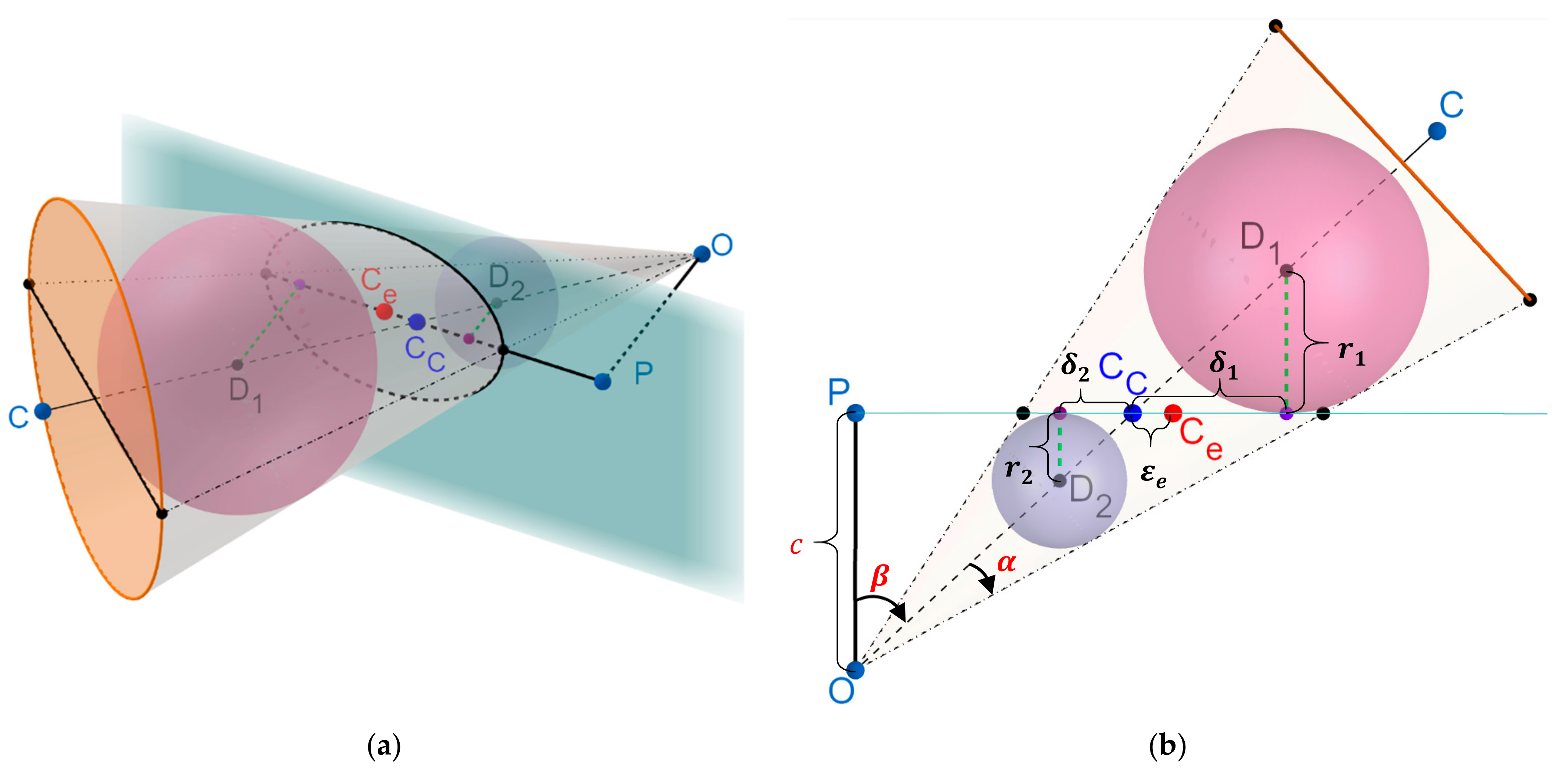
The ellipse formed by the perspective projection of a sphere onto an image is equivalent to the ellipse formed by the intersection of the tangential cone to the sphere with the plane. Miller and Goldman [5] explained the relationship between a randomly oriented plane intersecting a cone. They showed that the centers of the two tangential Dendelin spheres (see Figure 1a,b), and the major axis of the generated ellipse, lie on a plane whose normal vector is parallel to the minor axis of the projected ellipse. As illustrated in Figure 1, the camera center, O , the centers of the Dandelin spheres, D 1 and D 2 , and the true center of the sphere, C , lie on the same line. The center of the sphere, projected onto the intersecting plane, C C , is, hence, the intersection of the line, connecting the centers of the Dendelin spheres with the major axis of the ellipse. Because the center of the ellipse, C e , is always on the major axis of the projected ellipse, the eccentricity error has only one component in the direction of the ellipse’s major axis, and no eccentricity in the direction of the orthogonal minor axis. To this end, the true target’s center in the image plane can be derived by translating the estimated ellipse’s center in the direction of the major axis by the eccentricity error, ε e , shown in Figure 1b.
To provide a closed-form solution for ε e , the following two relationships from [5] are employed:
r 1 r 2 = cos β + sin α cos β sin α   ,
b e = c · sin α cos 2 β sin 2 α   ,
where r 1 and r 2 are the radii of the two tangential Dandelin spheres, α is the half-angle of the cone, β is the angle between the cone’s axis and the intersecting plane’s normal, b e is the semi-minor length of the best fit ellipse, and c is the camera’s principal distance (focal length). Using the notations of Figure 1b, the eccentricity error, ε e , can be derived as follows:
ε e = f e δ 2   where   f e = a e 2 b e 2 ,
where a e is the semi-major length of the best fit ellipse, f e is the distance of the ellipse’s center to one of the focal points, and δ 2 is shown in Figure 1b. Based on the similarity of the two right angled triangles, we have:
δ 2 δ 1 = r 2 r 1     Substituting   Equation   1     δ 2 δ 1 = cos β sin α cos β + sin α         δ 2 δ 1 + δ 2 = cos β sin α 2 cos β δ 1 + δ 2 = 2 f e                 δ 2 = f e f e sin α cos β ,
The ratio sin α cos β can be directly derived from Equation (2):
sin α cos β = 1 1 + c b e 2   ,
Substituting Equations (5) and (4) into Equation (3) provides the closed-form solution to the magnitude of the eccentricity error:
ε e = f e 1 + c b e 2   ,
The ellipse center must now be translated onto the major axis with magnitude ε e . The direction of the translation, as observed in Figure 1, must always be towards the principal point, P . Equation (6) also shows that the eccentricity is zero when the focal length of the projected ellipse is zero (the ellipse is a circle). This occurs in the marginal case when the estimated ellipse center lies exactly on the principal point. The latter can be geometrically explained from the following generic relationships:
  • The cone’s vertex, and the two centers of the Dandelin spheres, always lie on the line passing through the center of the cone’s base.
  • The two Dandelin spheres are also tangential (orthogonal) to the ellipse’s major axis at the focal points.
  • The line connecting the cone’s vertex and the center of the ellipse is also orthogonal to the ellipse’s major axis (marginal case of center passing through the principal point).
  • Because the spheres’ centers lie on one side of the cone’s vertex, and the ellipse’s center lies between the two focal points, the only acceptable arrangement is when the center and the focal points are the same, which suggests no eccentricity.
  • Condition 4 can only hold if Condition 3 is satisfied. Condition 3 can only occur as a special case when the camera’s optical axis passes through the sphere’s center, which is expected to produce no eccentricity error [3]. As mentioned, in this case, the projection of the sphere onto the image plane will be a circle.
From Condition 3, it can be inferred that the major axis of the projected ellipse also passes through the camera’s principal point. Predicated on the aforementioned discussions, the corrected image coordinates of the spherical target center, x c e , y c e are obtained using Algorithm 1, given the camera’s principal distance, c , and principal point, P = x p , y p , and the geometric parameters of a best fit ellipse, x e , y e , a e , b e , θ e , representing the ( x , y ) coordinates of the center, semi-major length, semi-minor length, and the major axis’ rotation angle in the image plane, respectively.
Algorithm 1 Corrected Ellipse Center
Inputs: Camera’s principal distance, c , principal point, P = x p , y p , best fit ellipse geometric parameters, x e , y e , a e , b e , θ e .
Output: Corrected center of the ellipse, x c e , y c e .
  • Calculate the distance vector from the ellipse’s center to the principal point:
    d p e = x p x e 2 + y p y e 2   ,
  • If d p e = 0 , x c e , y c e = x e , y e , and exit the algorithm.
  • Else, perform the following steps:
    3.1.
    Determine the unit vector representing the direction of the major axis:
    a c e = cos θ e , sin θ e   ,
    3.2.
    Calculate the focal point of the ellipse, f e = a e 2 b e 2 .
    3.3.
    Estimate the magnitude of the eccentricity error, ε e , using Equation (6).
    3.4.
    Estimate the corrected ellipse center, x c e , y c e , using the following equation:
    x c e = x e ε e · cos θ e y c e = y e ε e · sin θ e   ,
Algorithm 1 requires an estimate of the interior orientation parameters (IOPs) of the camera, c , and P . This initial estimate can be obtained from pre-calibration [8,
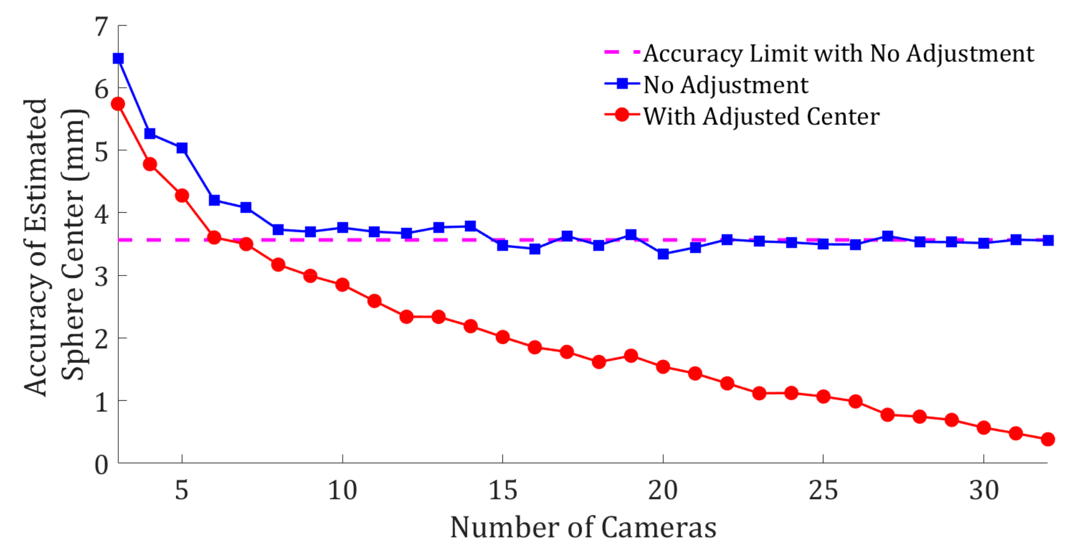
9], manufacturer’s specifications, or the Exchangeable Image File (EXIF). In addition, it is possible to use Algorithm 1 to help correct camera positions in applications involving tracking spheres using cameras. In case the application involves tracking, say, a rigid spherical ball, the corrected center can be used to guide the direction of the movement of the camera to always face the center of the ball (i.e., the only position with no eccentricity error).

2.2. Data Collection and Validation

A white Styrofoam spherical target on a black background was attached to the wall as the subject of the main experiment presented in this study (Figure 2a). The true radius of the spherical target was 50 mm (to 0.01 mm measurement precision). The color contrast between the spherical target and its background were purposefully designed to guarantee a clear detectable boundary for the ellipse representing the projected sphere on the image. In each image, an ellipse is fitted to the boundary of the sphere using the reliable confocal hyperbola ellipse fitting method proposed in [10]. The center of the best fit ellipse is then adjusted using Algorithm 1 (Figure 2b).
A pre-calibrated Huawei P30 mobile phone camera was used to acquire thirty-two 4K images of the spherical target. The calibration of the smartphone camera was performed using the method and IOPs presented in [9]. The position and orientation of the camera for each image view (exterior orientation parameters) were estimated automatically (independent of the spherical target’s center) using COLMAP [11], a reliable open source structure-from-motion [12] software. The camera positions are shown in Figure 2c with red pyramids. Figure 2d shows the point cloud of the target after dense 3D reconstruction. Figure 2e shows the best fit sphere (shown in green) to the point cloud of the spherical target. The center of the best fit sphere is then used as ground truth in the presented analysis. The reconstruction object space scale is defined using the ratio between the real-world and the best fit radius of the spherical target.

2.3. Robust Sphere Detection in 3D Point Clouds

The validation of the estimated 3D reconstructed center of the sphere for the experiment presented in Section 2.2 is predicated on an accurate and reliable methodology to fit spheres to 3D reconstructed point clouds. To this end, a new methodology for robust fitting of spheres to 3D point clouds was developed. The proposed method extends the direct hyperaccurate least squares circle fit of Chernov [13,14] to spheres. The extension of Chernov’s hyperaccurate method was combined with the robust model fitting algorithm of Maalek, presented in Appendix B (Algorithm A1) of [15] to minimize the impact of outliers on the estimated sphere parameters (i.e., radius and center). The hyperaccurate direct circle fitting to 2D points was extended here for fitting spheres to 3D points because the original method was proven to eliminate the essential bias of the estimated radius of the best fit circle [14]. The new extension to the direct hyperaccurate sphere fitting is presented in Algorithm 2 using singular value decomposition to provide optimal numerical stability [
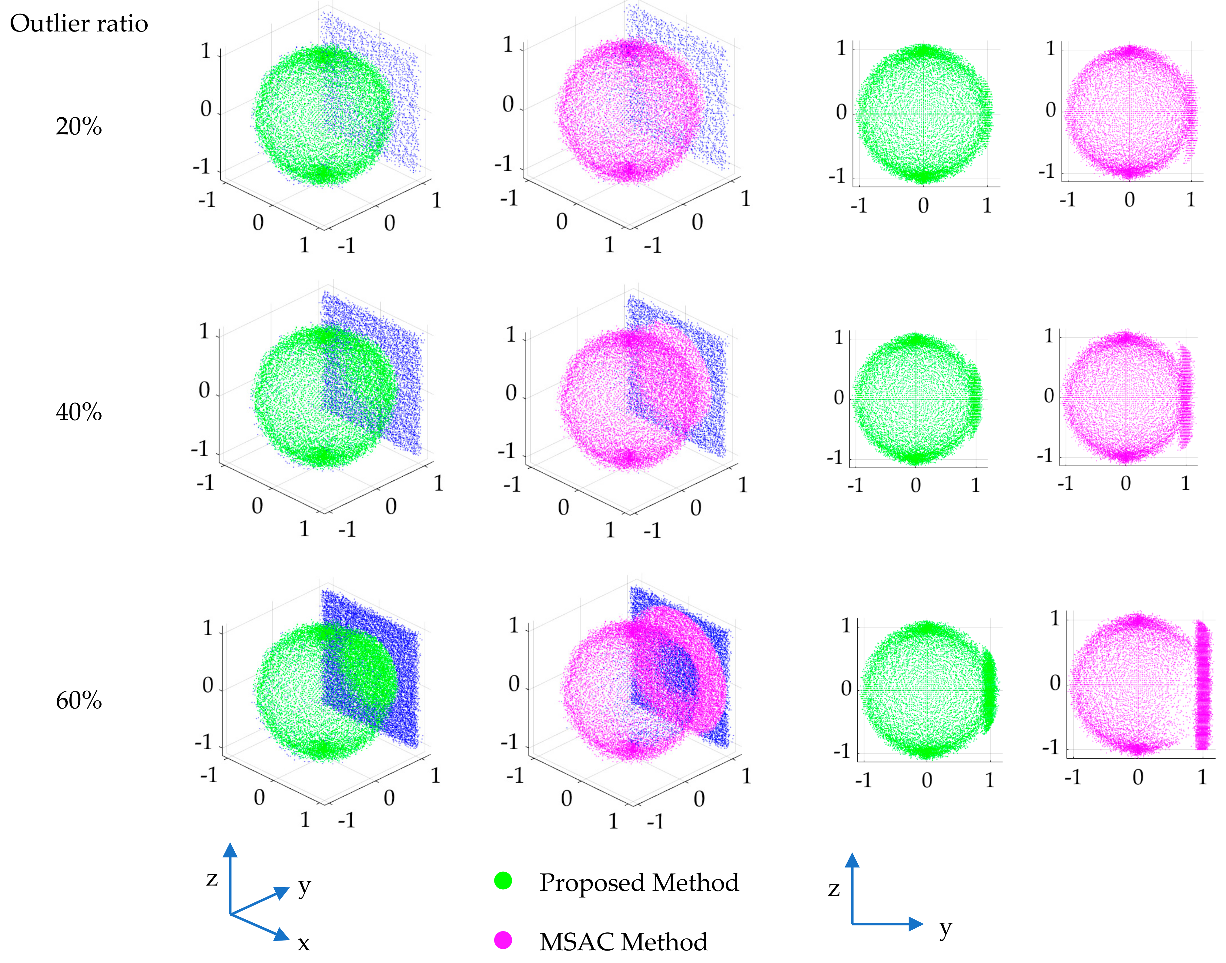
14]. Furthermore, reliable outlier detection is key because it provides the necessary basis to fit the sphere to only the spherical points and eliminate the adverse effects of outliers on the estimated sphere parameters. The methodology of Maalek for outlier detection was utilized here because this method was shown to be superior to popular robust methodologies, such as random sample and consensus (RANSAC) shape detection [15] as well as the least trimmed squared (LTS) method in linear regression [16]. The hyperaccurate circle fitting together with Maalek’s outlier detection method was also proven reliable for robust circle and cylinder fitting to 3D point clouds [16,
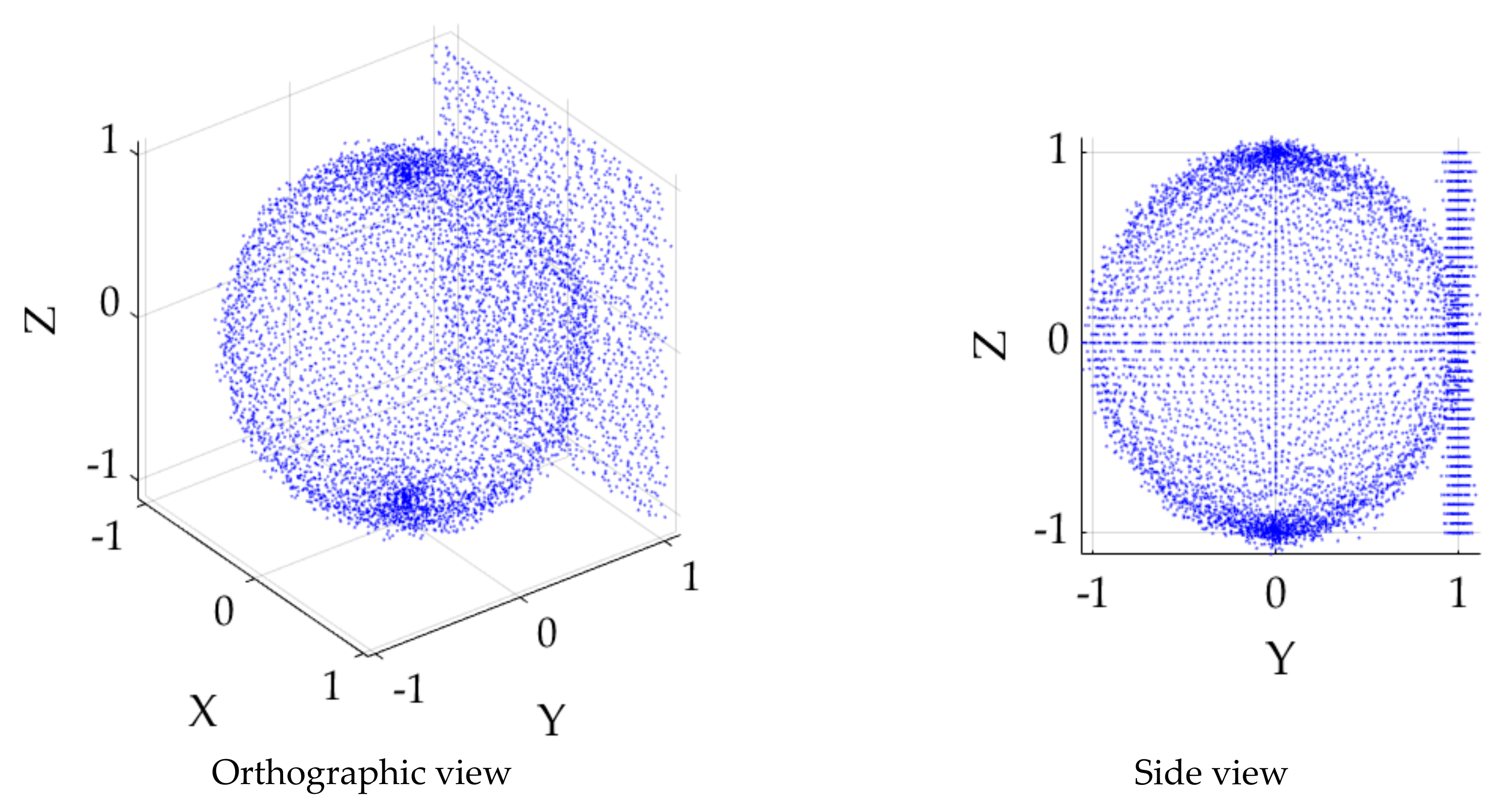
17]. It is, hence, hypothesized that this method will produce reliable and robust sphere fitting results for the experiment presented in this study. The effectiveness of the newly proposed sphere fitting will also be investigated in this study on simulated point cloud datasets.
Algorithm 2 Hyperaccurate Direct Algebraic Sphere Fit
Inputs: Point cloud, X i = x i , y i , z i , i = 1 : n , where n is the number of observations.
Outputs: Estimated best fit least squares sphere’s radius, R , and center, C .
  • Calculate the mean of the observations X ¯ = x ¯ , y ¯ , z ¯ .
  • Compute w i = x i x ¯ 2 + y i y ¯ 2 + z i z ¯ 2 for ( i = 1 : n ).
  • Construct the Z matrix as follows:
    Z = w 1 x 1 x ¯ y 1 y ¯ w n x n x ¯ y n y ¯ z 1 z ¯ z n z ¯ 1 1   ,
  • Perform the singularvalue decomposition on Z = U D V T .
  • Calculate the algebraic parameter vector of the best fit sphere, A , as follows:
    5.1.
    If D 5 , 5 D 1 , 1 ϵ (the singular case), set A = V : , 5 , where D i , j is the element corresponding the the i th row and j th column of D , V : , 5 is the vector corresponding to the 5th column of V , and A is the algebraic paramer vector of the sphere. ϵ = 10 12 is custumary for practical applications [14].
    5.2.
    Else, perform the following steps:
    5.2.1.
    Calculate the mean of the first column of Z : w ¯ = 1 n w i ( w i : defined in Step 2).
    5.2.2.
    Construct matrix G as follows:
    H = 0 0 0 0 1 2 0 1 0 0 0 0 0 1 0 0 0 0 0 1 0 1 2 0 0 0 2 w ¯   ,
    5.2.3.
    Calculate the matrix multiplication T = V S V T G V S V T using steps 4 and 6.2.
    5.2.4.
    Find the eigenvector, A * , corresponding to the smallest non-negative eigenvalue of T .
    5.2.5.
    Calculate the algebraic parameter vector of the sphere: A = V S 1 V T A * .
  • Use the following equations to calculate the radius, R , and center, C , of the sphere:
    R = A 2 2 + A 3 2 + A 4 2 4 A 1 A 5 2 A 1   ,
    C = X ¯ 1 2 A 1 A 2 A 3 A 4 ,
    where A i represents the i th element of the sphere’s algebraic parameter vector, A .

3. Experimental Design

In this study, two sets of experiments were carried out to evaluate the effectiveness of Algorithm 1 and Algorithm 2. The first experiment assessed the accuracy of the newly proposed sphere fitting method, compared to the reliable M-estimator sample consensus (MSAC) method of [18] for robust sphere detection on simulated datasets. The second experiment investigated the impact of modeling the eccentricity error in images on the 3D reconstructed center of spheres as the number of image views increase.

3.1. Experiment 1: Robust Sphere Fitting Evaluation

This experiment was designed to evaluate the effectiveness of Algorithm 2 in combination with Algorithm A1 of [15], compared to the MSAC method of [18] on simulated datasets. To this end, 50,000 sets of point cloud data corresponding to a unit sphere, attached to a planar surface with parameter vector γ = 0 , 1 , 0 , 1 , as per the planar parameter convention of [19], were simulated. The square unit planar patch was so chosen to simulate the arrangement of Figure 2a, while serving as the outlier set in each point cloud dataset (i.e., the ratio of outliers refers to the ratio of points generated on the planar patch to all generated points). At each simulation, the point cloud generation was performed while varying specific properties, namely, number of points (resolution), noise (as zero mean normally distributed error), and outlier ratio. The domains of the parameter selection (i.e., number of points, noise, and outlier ratio) are presented in Table 1. At each of the 50,000 simulations, a random configuration from Table 1 was selected to generate the point cloud. A sample of the dataset is provided in Figure 3.
For each simulated point cloud, the estimated radius and center of the sphere, along with the sphere detection quality, using our proposed and MSAC methods, were recorded. For the radius and center, the distance (L2-norm) between the actual and the estimated were calculated. To evaluate the quality of automatic detection of points following spherical patterns (sphere detection quality), the established metrics, namely, precision, recall, accuracy, and F-measure, were used, which are calculated as follows [20]:
P r e c i s i o n = T P T P + F P R e c a l l = T P T P + F N A c c u r a c y = T P + T N T P + T N + F P + F N F m e a s u r e = 2 · P r e c i s i o n · R e c a l l P r e c i s i o n + R e c a l l ,
where T P , T N , F P , F N are, respectively, the number of true positive, true negative, false positive, and false negatives, of the object detection method.

3.2. Experiment 2: Eccentricity Error Correction vs. Number of Images

This experiment investigated the impact of the modeled as well as the unmodeled eccentricity error on the accuracy of the 3D reconstructed sphere’s center. This impact was measured as the number of image views increase from two to thirty-two. Because different combination of views will provide different reconstruction results for a given number of (say k ) image views, N different combinations of k = 2 32 images are selected. To this end, for k image views, the following steps are carried out:
  • Randomly select N different combination of k images from the 32 images.
  • For each set of k images, using the estimated best fit ellipse center (unmodeled), adjusted center (modeled), and camera projection matrices (see Figure 2b,c), perform triangulation [21] and determine the object space position of both the adjusted centers and the best fit ellipse centers.
  • Calculate the Euclidian distance between the object space coordinates of the adjusted and unadjusted centers from the ground truth (Figure 2e).
  • For a given number of image views, k , record the mean of the N distances obtained from Step 3.
In our experiments, N = min 250 , 32 k is chosen.

4. Experimental Results and Discussions

4.1. Experiment 1: Robust Sphere Fitting Evaluation

As discussed in Section 3.1, three types of analysis, namely accuracy of the estimated radius, accuracy of the estimated center, and quality of the sphere point detection, were performed.

4.1.1. Experiment 1: Accuracy of the Estimated Radius

Figure 4 shows the results of the radius estimation accuracy using the proposed method and the MSAC methods for the 50,000 simulated point cloud datasets. The horizontal axis represents the absolute difference between the estimated and true radius (i.e., unit radius), while the vertical axis represents the cumulative probability. Figure 4 shows that the estimated radius using the proposed method considerably outperforms those estimated using the MSAC method. To provide a numerical comparison, the mean, median, and 95th percentile of the estimated radius for each method is presented in Table 2. The results presented in Table 2 show that the mean, median, and 95th percentile of the accuracy of the estimated radius using our method outperformed those of the MSAC method by a factor of approximately 12, 17, and 11, respectively.

4.1.2. Experiment 1: Accuracy of the Estimated Center

Figure 5 shows the cumulative probability distribution of the estimated center of the sphere using the proposed and MSAC methods. Similar to the radius estimation case, Figure 5 shows that the estimated center of the best fit sphere using the proposed methods significantly outperforms those estimated using the MSAC method. Table 3 shows the mean, median, and 95th percentile of the accuracy of the estimate center using both methods. The results of Table 3 indicate that the mean, median, and 95th percentile of the accuracy of the estimated center using our method improved those achieved using the MSAC method by a factor of 14, 17, and 12, respectively.
From the results of Table 3, together with Table 2, two important observations can be made. First, when comparing Table 2 and Table 3, it was observed that both methods produced more accurate radius estimation than center estimation. While the proposed method considerably outperformed the MSAC method, the radius was, on average, estimated almost 3 times better than the center in both methods. Second, Table 3 shows that, 95% of the time, the center of the Styrofoam target of interest with radius of 50 mm (Figure 2) is estimated better than 0.5 mm. This result is, of course, considering the noise levels of up to 5% of the radius of the sphere (simulation domain of Table 1). The noise level of the Styrofoam target was, however, in the order of 2% of the radius (obtained using the root mean squared error of the best fit sphere). At this noise level and considering the number of 3D reconstructed points and outlier ratio for the Styrofoam target, the simulation results indicated that the center of the Styrofoam target was estimated better than 0.1 mm, 100% of the time. This, however, was significantly larger using the MSAC method, which achieved better than 5mm center estimation 100% of the time. As will be revealed in Section 4.2, the center estimation accuracy of 0.1 mm achieved using the proposed method is sufficient, whereas the accuracy of 5 mm achieved using the MSAC will be inadequate.

4.1.3. Experiment 1: Quality of Sphere Detection

The quality of the robust spherical point detection is calculated using Equation (14) for both the proposed and MSAC methods. The precision, recall, accuracy, and F_Measure were calculated using the number of correct and incorrect detections in all simulations combined. The results of the sphere detection quality are presented in Table 4. As observed, the two methods achieved similar results in terms of precision, which is an indicator of Type I errors (i.e., spherical points not detected as spherical). The proposed method, however, achieved recall of around 15% points more than the MSAC, which is an indication of robustness to Type II errors (i.e., points of the planar patch incorrectly detected as sphere; Figure 6). A similar trend in accuracy and F_Measure was observed, indicating the superior performance of the proposed method compared to the MSAC.
Figure 6 shows the results of the sphere detection using the proposed and MSAC methods for a sample sphere and plane point cloud for 10,000 points and noise level of 0.05 with outlier ratios of 20%, 40%, and 60%. It can be observed that, as the outlier ratio increases, the MSAC method includes many points of the planar patch as spherical. This trend was much less evident using the proposed method, which achieved satisfactory results. The latter phenomenon, i.e., the inclusion of points of the planar patch as spherical, is the reason for the lower recall rates of the MSAC method compared to the proposed method (as reported in Table 4).

4.2. Experiment 2: Eccentricity Error Correction vs. Number of Images

Figure 7 shows the accuracy of the 3D reconstruction of the spherical target using adjusted as well as the unadjusted center in images as a function of the number of image views. Two important observations can be made from Figure 7. Firstly, the accuracy of the estimated center of the sphere using the adjusted centers (the red curve) consistently falls below that without using center adjustment (the blue curve). This suggests that the average accuracy obtained using the adjusted center outperforms that without center adjustment.
Secondly, it was observed that the accuracies of the estimated centers—for both modeled and unmodeled eccentricity—are improved (almost with the same slope) as the number of image views increases from two to eight. At around eight image views, the accuracy of the centers estimated using the center of the best fit ellipse (unadjusted eccentricity error) remains (almost) constant as the number of image views increase (shown with the hidden line in Figure 7). This, however, is not the case when the center in each image is adjusted using Algorithm 1. In fact, as the number of image views increase, the accuracy of the estimated center is consistently improving. The accuracy using the unadjusted and adjusted centers improved by 46% and 93% on average, respectively, when the number of image views changed from two to thirty-two. Using all thirty-two images, the accuracy of the estimated center is improved by over an order of magnitude using our proposed eccentricity adjustment method (accuracy of around 0.25 mm vs. 3.5 mm for adjusted and unadjusted errors, respectively). The results of this study corroborate the importance of modeling the eccentricity errors as well as the effectiveness of our derived formulation to correctly model this phenomenon.

5. Discussions and Conclusions

The closed form solution for the eccentricity error of the center of a spherical target, projected into an image, was derived. The effectiveness of the proposed formulation in estimating the 3D coordinates of the center of a spherical target was examined. The accuracy was quantified as the number of image views increased from two to thirty-two. It was shown that the accuracy of the estimated center using the center adjustment was better than that without center adjustment (i.e., using the best fit ellipse center). The accuracy of the estimated center using the adjusted center and without adjustment improved by 93% and 46% on average, respectively, as the number of image views increased from two to thirty-two. It was also revealed that the accuracy of the estimated 3D center without eccentricity adjustment did not improve noticeably as the number of image views increased from eight to thirty-two. This was, in fact, not the case for the estimated centers with the eccentricity adjustment, whose accuracy continuously improved as the number of image views increased. The negative impact of unmodeled eccentricity error in simulated stereopairs was demonstrated in Luhmann [3]. In this study, we observed that not only must this eccentricity error be modeled, but also the eccentricity adjustment becomes even more crucial as the number of image views increase (say for multi-camera systems).
To reliably conclude the main results presented in Figure 7, the accuracy of the estimated center of the Styrofoam target must be better than the 0.25 mm. The 0.25 mm was the distance between the ground truth sphere’s center and the center estimated by first correcting the eccentricity in all 32 images and then #d reconstruction through triangulation. This, hence, required a best fit sphere method that can provide center estimation better than the 0.25 mm in the presence of outlying observations. To this end, a new robust sphere fitting method was proposed, which combined the idea of Chernov for circle fitting [14] together with Maalek’s robust model fitting method [15]. The newly proposed method at the noise level, outlier ratio, and number of points corresponding to the dense 3D reconstructed Styrofoam target achieved an accuracy of better than 0.1 mm, which satisfied the 0.25 mm accuracy requirement. The MSAC method, on the other hand, could only provide a center estimation accuracy of within 5 mm, which would be unsatisfactory for the experiment presented in this study. This demonstrates the importance of the proposed method for robust sphere fitting from point clouds in the presence of outlying observations.

Author Contributions

Conceptualization, R.M.; methodology, R.M.; software, R.M.; validation, R.M. and D.D.L.; formal analysis, R.M.; investigation, R.M.; resources, R.M. and D.D.L.; data curation, R.M.; writing—original draft preparation, R.M.; writing—review and editing, R.M. and D.D.L.; visualization, R.M.; supervision, R.M. and D.D.L.; project administration, R.M. and D.D.L.; funding acquisition, R.M. All authors have read and agreed to the published version of the manuscript.

Funding

The authors wish to acknowledge the support provided by the KIT Publication Fund of the Karlsruhe Institute of Technology in supplying the APC. This research received no additional external funding.

Institutional Review Board Statement

Not applicable.

Data Availability Statement

The data presented in this study are available upon request from the author. Please visit the website for the Department of Digital Engineering and Construction at https://www.tmb.kit.edu/english/Mitarbeiterseite_5850.php (accessed on 17 August 2021) or contact the author directly via email at [email protected].

Acknowledgments

The authors would like to thank the late mathematician, Nikolai Chernov (10 November 1956–7 August 2014), whose outstanding masterpiece, titled, Circular and Linear Regression: Fitting Circles and Lines by Least Squares, inspired the development of the new sphere fitting algorithm (Algorithm 2), presented in this study.

Conflicts of Interest

The authors unequivocally declare no conflict of interest.

References

  1. Ahn, S.J.; Warnecke, H.J.; Kotowski, R. Systematic Geometric Image Measurement Errors of Circular Object Targets: Mathematical Formulation and Correction. Photogramm. Rec. 1999, 16, 485–502. [Google Scholar] [CrossRef]
  2. FIFA Quality. FIFA Quality Programme for Goal-Line Technology Testing Manual; Fédération Internationale de Football Association (FIFA): Zurich, Switzerland, 2014. [Google Scholar]
  3. Luhmann, T. Eccentricity in images of circular and spherical targets and its impact on spatial intersection. Photogramm. Rec. 2014, 29, 417–433. [Google Scholar] [CrossRef]
  4. Lichti, D.D.; Glennie, C.L.; Jahraus, A.; Hartzell, P. New Approach for Low-Cost TLS Target Measurement. J. Surv. Eng. 2019, 145, 04019008. [Google Scholar] [CrossRef]
  5. Miller, J.; Goldman, R. Using tangent balls to find plane sections of natural quadrics. IEEE Eng. Med. Biol. Mag. 1992, 12, 68–82. [Google Scholar] [CrossRef]
  6. Hohenwarter, M.; Jarvis, D.; Lavicza, Z. Linking Geometry, Algebra and Mathematics Teachers: GeoGebra Software and the Establishment of the International GeoGebra Institute. Int. J. Technol. Math. Educ. 2009, 16, 83–87. [Google Scholar]
  7. Botana, F.; Hohenwarter, M.; Janičić, P.; Kovács, Z.; Petrović, I.; Recio, T.; Weitzhofer, S. Automated Theorem Proving in GeoGebra: Current Achievements. J. Autom. Reason. 2015, 55, 39–59. [Google Scholar] [CrossRef]
  8. Lichti, D.D.; Jarron, D.; Tredoux, W.; Shahbazi, M.; Radovanovic, R. Geometric modelling and calibration of a spherical camera imaging system. Photogramm. Rec. 2020, 35, 123–142. [Google Scholar] [CrossRef]
  9. Maalek, R.; Lichti, D.D. Automated calibration of smartphone cameras for 3D reconstruction of mechanical pipes. Photogramm. Rec. 2021, 36, 124–146. [Google Scholar] [CrossRef]
  10. Maalek, R.; Lichti, D.D. New confocal hyperbola-based ellipse fitting with applications to estimating parameters of mechanical pipes from point clouds. Pattern Recognit. 2021, 116, 107948. [Google Scholar] [CrossRef]
  11. Schönberger, J.L. Robust Methods for Accurate and Efficient 3D Modeling from Unstructured Imagery; ETH Zurich: Zurich, Switzerland, 2018. [Google Scholar]
  12. Ullman, S. The interpretation of structure from motion. Proc. R. Soc. Lond. Ser. B Biol. Sci. 1979, 203, 405–426. [Google Scholar] [CrossRef]
  13. Al-Sharadqah, A.; Chernov, N. Error analysis for circle fitting algorithms. Electron. J. Stat. 2009, 3, 886–911. [Google Scholar] [CrossRef]
  14. Chernov, N. Circular and Linear Regression; CRC Press: Boca Raton, FL, USA, 2010. [Google Scholar]
  15. Maalek, R. Field Information Modeling (FIM)™: Best Practices Using Point Clouds. Remote Sens. 2021, 13, 967. [Google Scholar] [CrossRef]
  16. Maalek, R.; Lichti, D.D.; Walker, R.; Bhavnani, A.; Ruwanpura, J.Y. Extraction of pipes and flanges from point clouds for automated verification of pre-fabricated modules in oil and gas refinery projects. Autom. Constr. 2019, 103, 150–167. [Google Scholar] [CrossRef]
  17. Maalek, R.; Lichti, D.D.; Maalek, S. Towards automatic digital documentation and progress reporting of mechanical construction pipes using smartphones. Autom. Constr. 2021, 127, 103735. [Google Scholar] [CrossRef]
  18. Torr, P.; Zisserman, A. MLESAC: A New Robust Estimator with Application to Estimating Image Geometry. Comput. Vis. Image Underst. 2000, 78, 138–156. [Google Scholar] [CrossRef] [Green Version]
  19. Maalek, R.; Lichti, D.D.; Ruwanpura, J.Y. Robust Segmentation of Planar and Linear Features of Terrestrial Laser Scanner Point Clouds Acquired from Construction Sites. Sensors 2018, 18, 819. [Google Scholar] [CrossRef] [PubMed]
  20. Olson, D.L.; Delen, D. Advanced Data Mining Techniques; Springer Science and Business Media LLC: Berlin, Germany, 2008. [Google Scholar]
  21. Hartley, R.; Zisserman, A.; Faugeras, O. Multiple View Geometry in Computer Vision, 2nd ed.; Cambridge University Press: Cambridge, UK, 2004; ISBN 978-0-521-54051-3. [Google Scholar]
Figure 1. Geometry of the intersection of a plane and a cone: (a) 3D orthographic view; (b) projected onto the plane whose normal vector is parallel to the minor axis of the intersecting ellipse. The images were generated using GeoGebra, a dynamic geometry, mathematics, and algebra software [6,7].
Remotesensing 13 03269 g001
Figure 2. (a) Spherical target with black background; (b) best fit ellipse, its center and the corrected center using Algorithm 1 for the image of the spherical target; (c) plan-view of the estimated position and orientation of each image; (d) dense 3D reconstruction of the spherical target; and (e) robust best fit sphere (shown in green).
Remotesensing 13 03269 g002
Figure 3. Simulated 3D point cloud of a unit sphere with the tangential plane in orthographic (left) and side (right) views.
Remotesensing 13 03269 g003
Figure 4. Cumulative probability distribution of the accuracy of the estimated radius of the 50,000 simulated point cloud configurations using the MSAC and proposed methods.
Remotesensing 13 03269 g004
Figure 5. Cumulative probability distribution of the accuracy of the estimated center of the 50,000 simulated point cloud configurations using the MSAC and proposed methods.
Remotesensing 13 03269 g005
Figure 6. Results of the detected spherical points with outlier ratios of 20%, 40%, and 60% using the proposed (green) and MSAC (magenta) methods in orthographic (left) and side (right) views.
Remotesensing 13 03269 g006
Figure 7. Accuracy of the estimated 3D reconstructed target centers using modeled eccentricity (with adjustment) as well as unmodeled (no adjustment), vs. the number of image views.
Remotesensing 13 03269 g007
Table 1. Domain of parameters used to simulate spheres (inliers) and tangential planes (outliers).
Configuration CategoryParameter Selection Domain
FromTo
number of points10010,000
noise00.05
outlier ratio10%60%
Table 2. Mean, median, and 95th percentile of the accuracy of the estimated radius using the proposed and MSAC methods.
StatisticAccuracy of Radius Estimation
ProposedMSAC
mean0.0020.022
median0.0010.013
95th percentile0.0070.074
Table 3. Mean, median, and 95th percentile of the accuracy of the estimated center using the proposed and MSAC methods.
StatisticAccuracy of Radius Estimation
ProposedMSAC
mean0.0040.057
median0.0030.045
95th percentile0.0130.151
Table 4. Mean, median, and 95th percentile of the accuracy of the estimated center using the proposed and MSAC methods.
MethodPrecision (%)Recall (%)Accuracy (%)F_Measure (%)
proposed96.2695.2194.1895.44
MSAC96.7080.9384.2387.79
Publisher’s Note: MDPI stays neutral with regard to jurisdictional claims in published maps and institutional affiliations.

