
On the Value of Sentinel-1 InSAR Coherence Time-Series for Vegetation Classification


Abstract
:1. Introduction
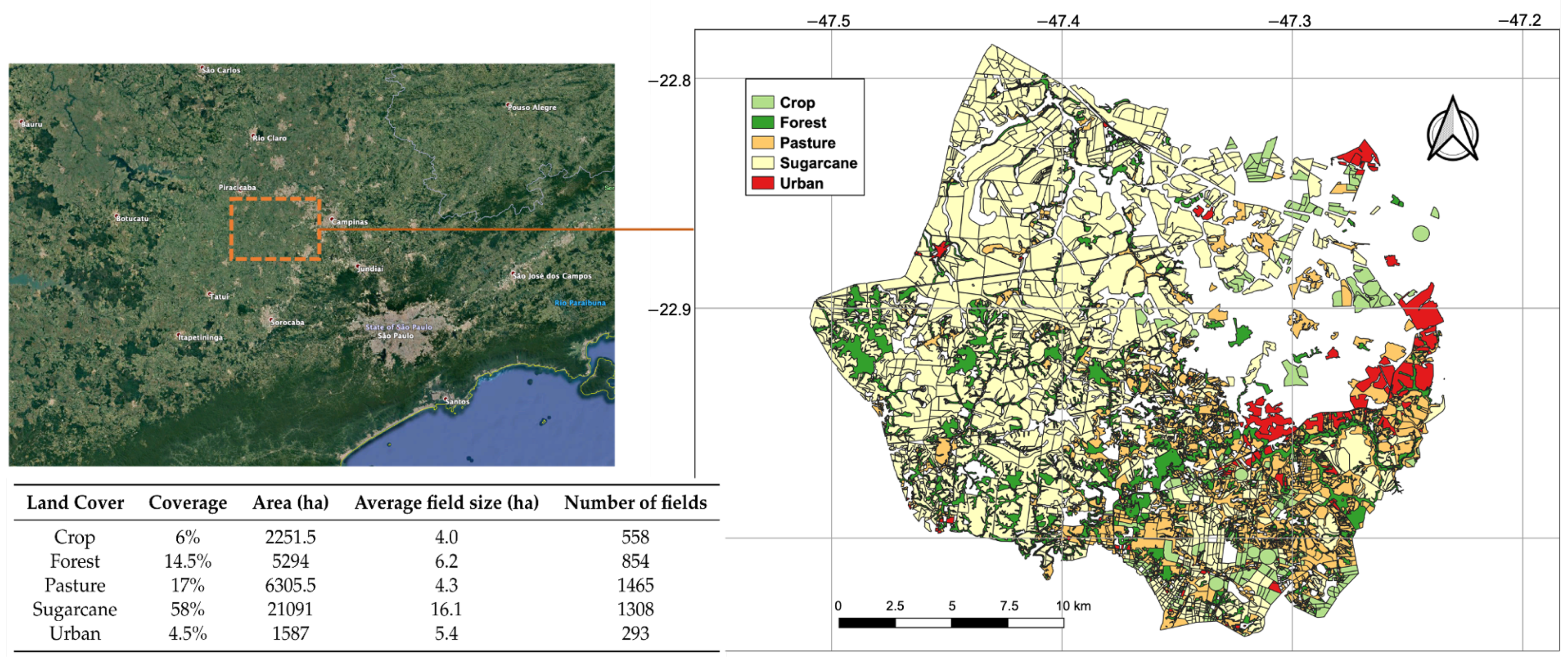
2. Study Area and Data
3. Methods
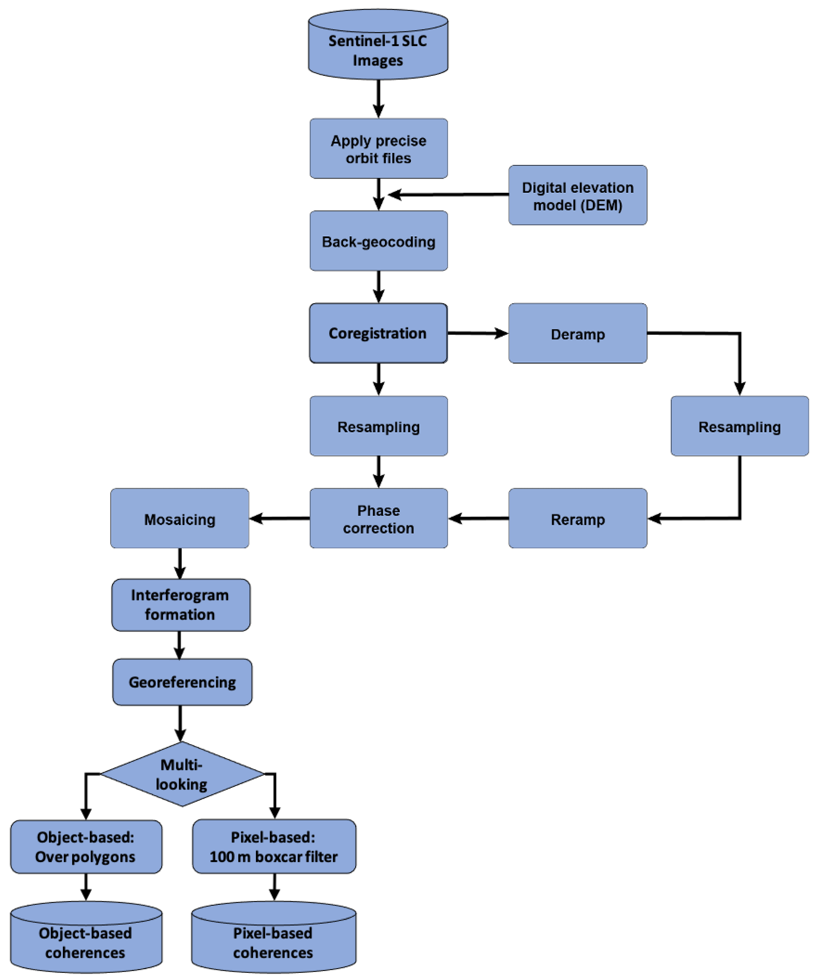
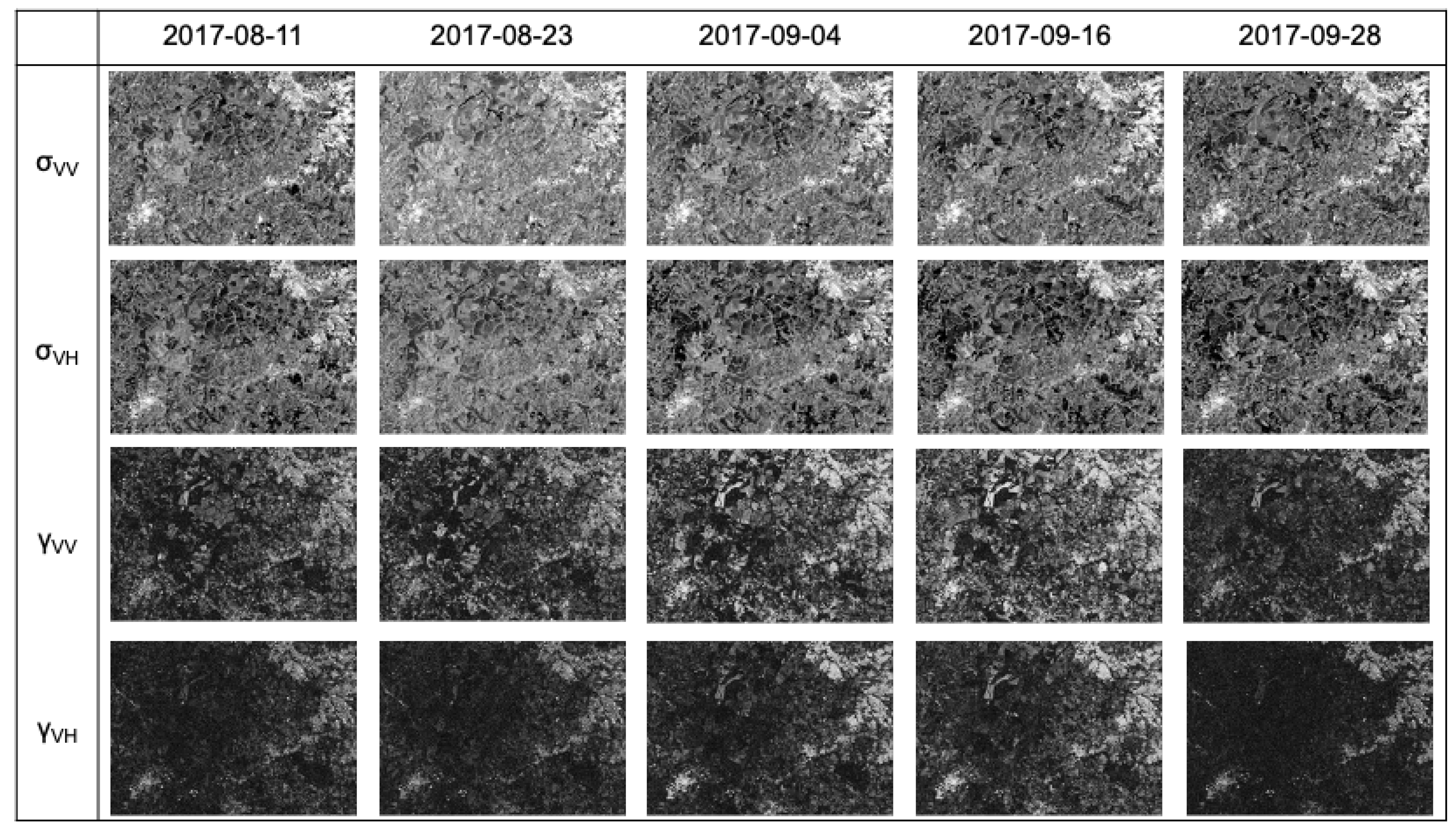
3.1. Pre-Processing
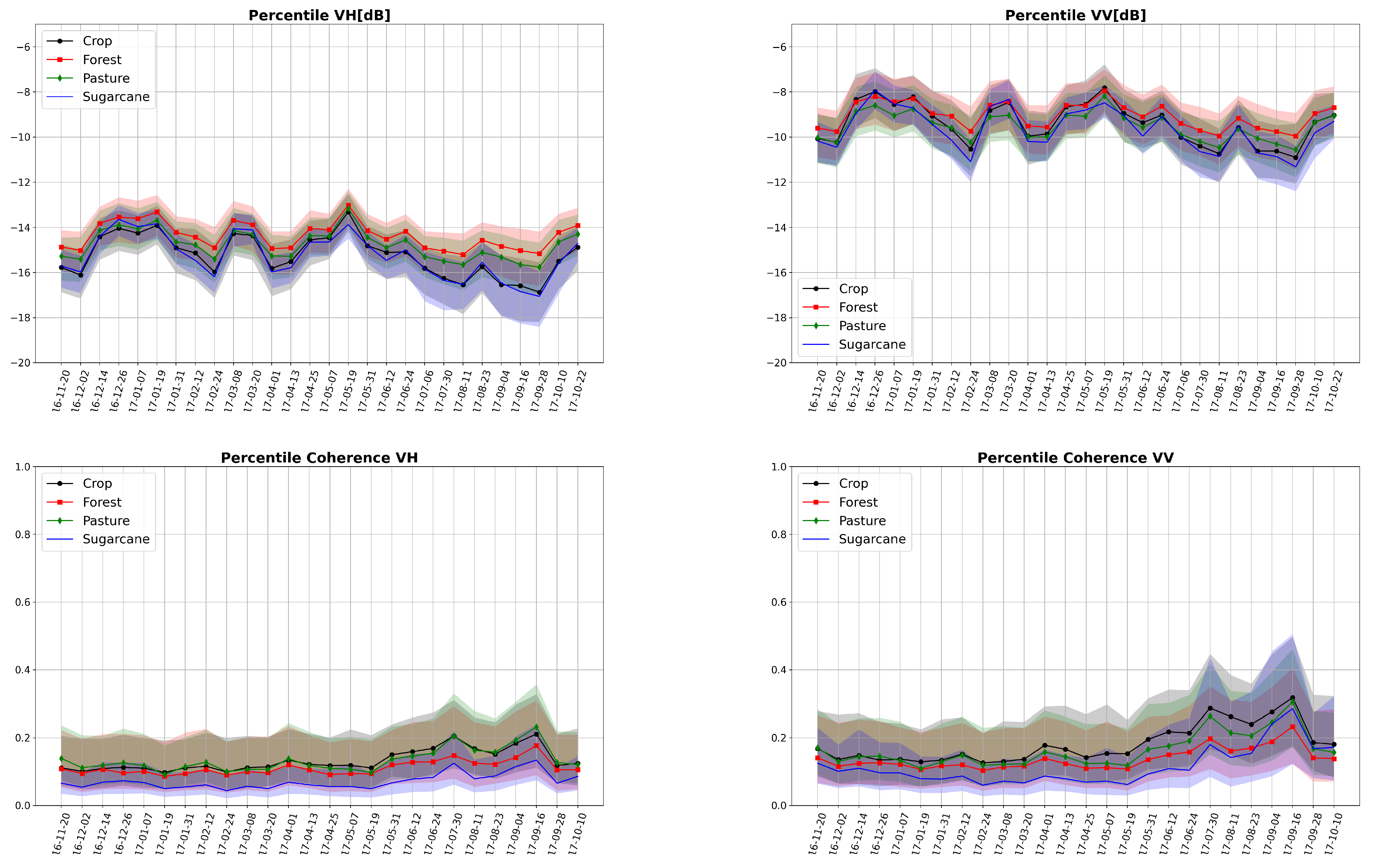
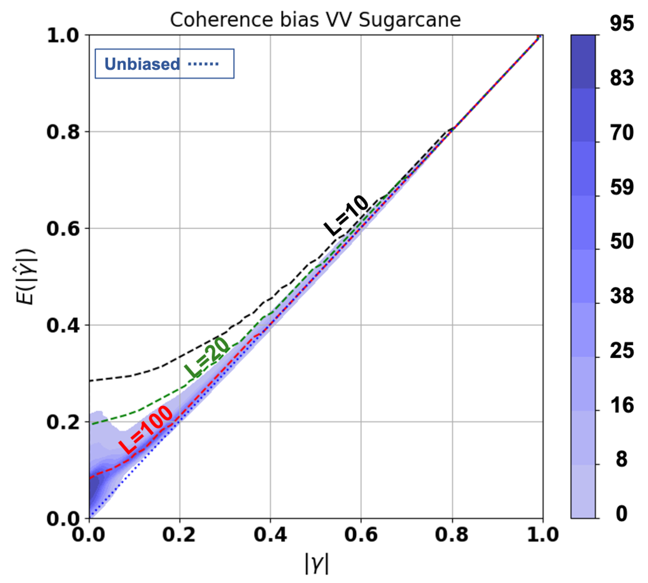
3.2. Interferometric Coherence
3.3. Land Cover Classification
- Random-Pixel Sampling: The pixel samples are randomly assigned to the training and validation sets without any spatial context constraint. The outcome is that any arbitrary field is allowed to have part of its pixels in the training set and part in the validation set. This is expected to lead to a positive bias in accuracy due to eventual overfitting, which occurs when the intra-polygon variability is lower than the variability between polygons of the same class. The risk in this random sampling approach is therefore that the algorithm learns the behavior of the individual fields rather than modeling their common statistical traits.
- Field-Pixel Sampling: In this approach, the pixels from the same polygon are entirely assigned either to the training or the validation set. For each class, the training set is built by iterative growth, i.e., by adding a field at a time to the set until 70% of the total pixels are allocated. The pixels from the excluded fields are assigned to the validation set.
- Field Sampling: This refers to object-based classification, as the samples correspond to the polygons themselves. The coherence magnitude and the backscatter intensity features are computed through multi-looking over the entire field. The differences with the field-pixels sampling are found in the impact of intra-field heterogeneities and in the different sensitivity to speckle noise. We are using the digitalized polygons (or objects or segments) from our ground surveying activities.
3.4. Feature Relevance
4. Results and Discussion
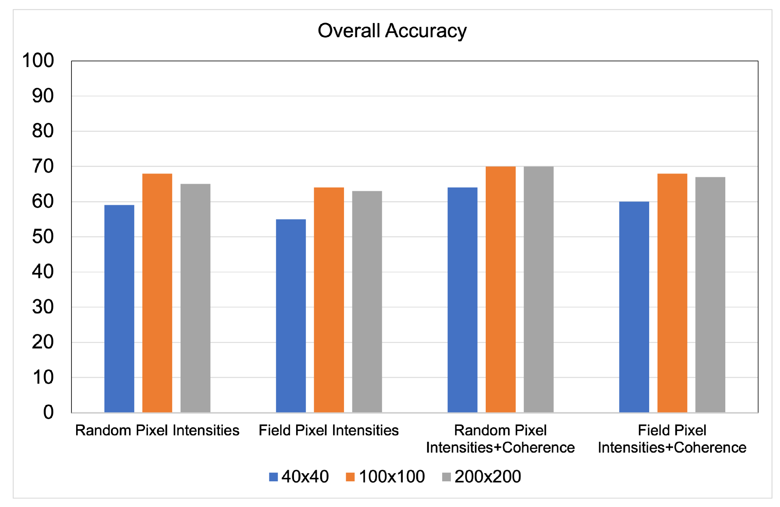
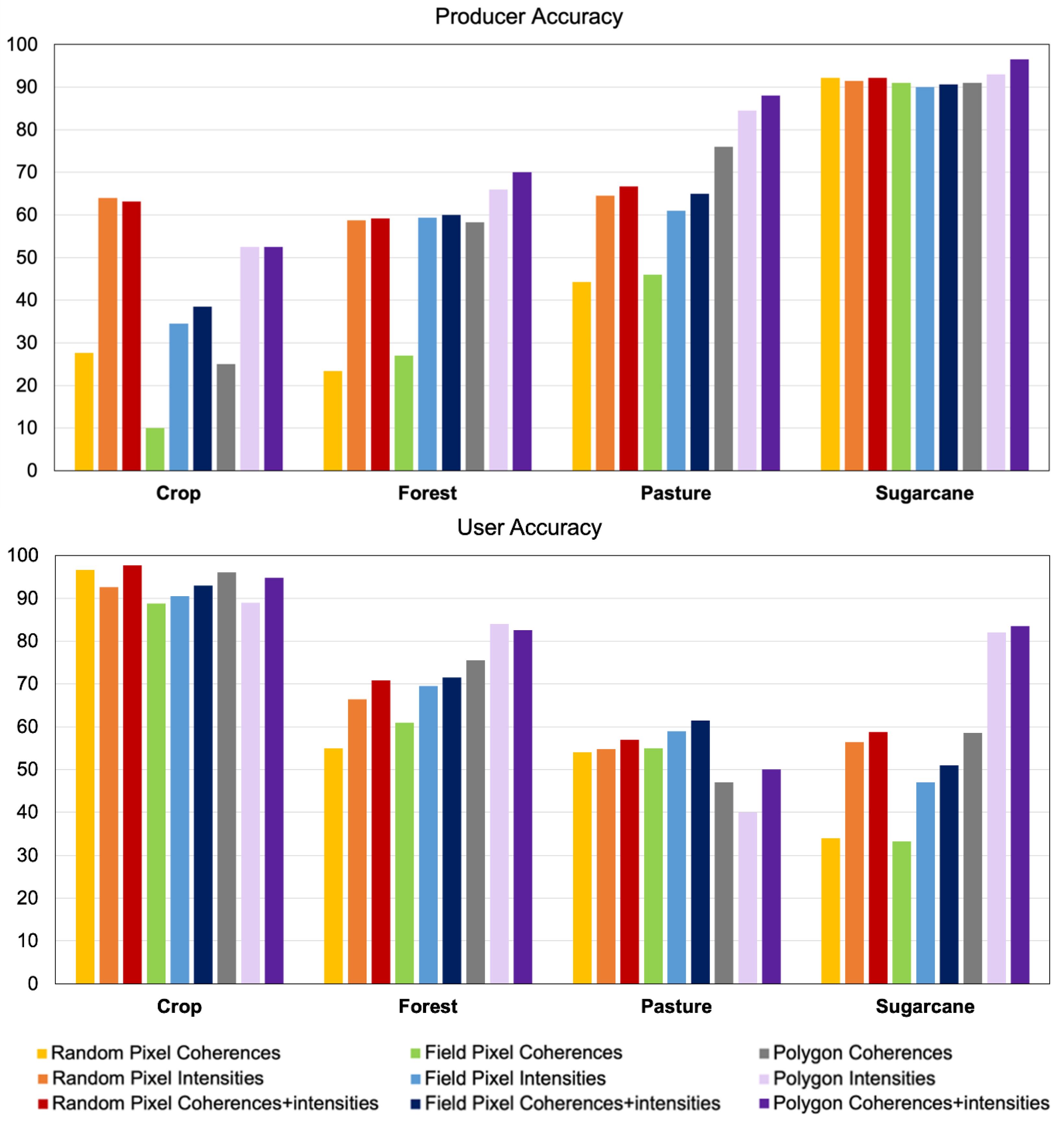
4.1. Quantitative Accuracy
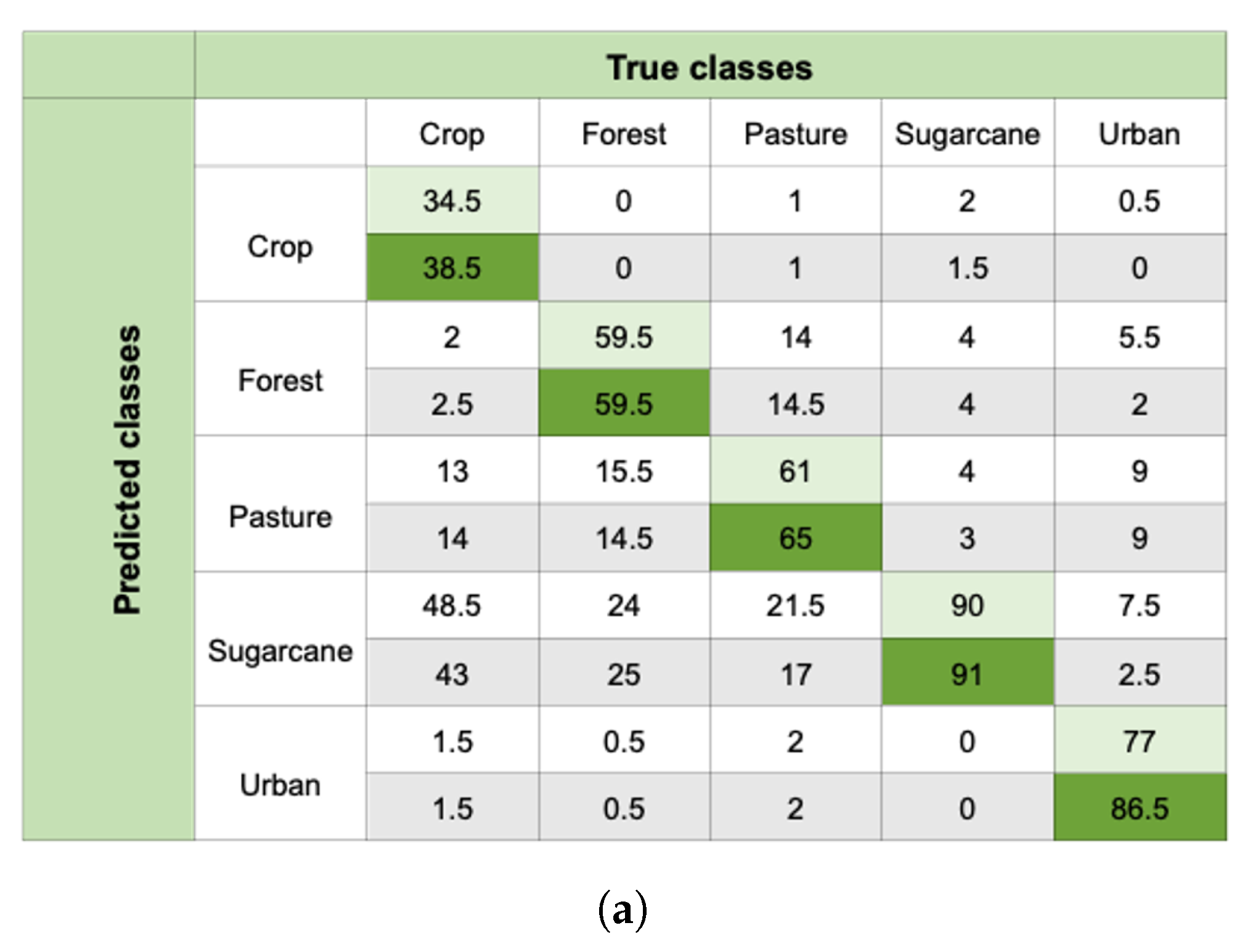
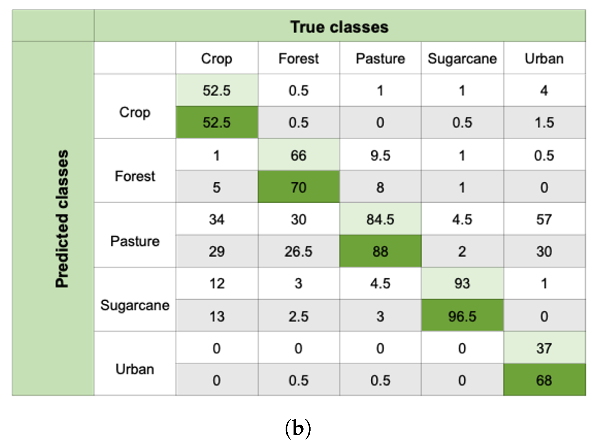
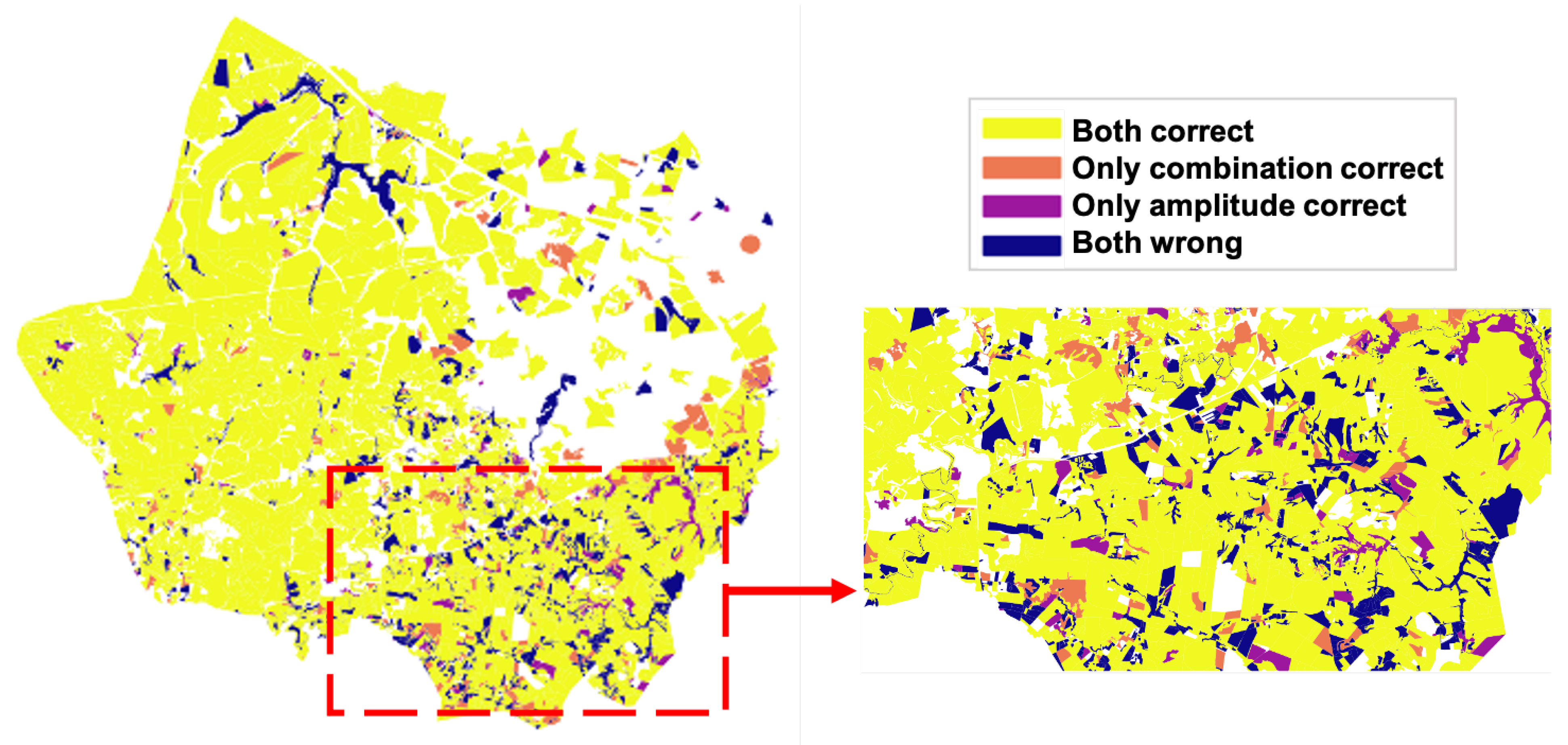
4.2. Spatial Analysis
4.3. Feature Relevance Analysis
5. Conclusions
Author Contributions
Funding
Institutional Review Board Statement
Informed Consent Statement
Acknowledgments
Conflicts of Interest
References
- Strozzi, T.; Dammert, P.; Wegmuller, U.; Martinez, J.M.; Askne, J.; Beaudoin, A.; Hallikainen, N. Landuse Mapping with ERS SAR Interferometry. IEEE Trans. Geosci. Remote Sens. 2000, 38, 766–775. [Google Scholar] [CrossRef]
- Bruzzone, L.; Marconcini, M.; Wegmuller, U.; Wiesmann, A. An Advanced System for the Automatic Classification of Multitemporal SAR Images. IEEE Trans. Geosci. Remote Sens. 2004, 42, 1321–1334. [Google Scholar] [CrossRef]
- Torres, R.; Snoeij, P.; Geudtner, D.; Bibby, D.; Davidson, M.; Attema, E.; Potin, P.; Rommen, B.; Floury, N.; Brown, M.; et al. GMES Sentinel-1 Mission. Remote Sens. Environ. 2012, 120, 9–24. [Google Scholar] [CrossRef]
- Rodriguez-Galiano, V.F.; Ghimire, B.; Rogan, J.; Chica-Olmo, M.; Rigol-Sanchez, J.P. An Assessment of the Effectiveness of a Random Forest Classifier for Land-Cover Classification. ISPRS J. Photogramm. Remote Sens. 2012, 67, 93–104. [Google Scholar] [CrossRef]
- Shao, Y.; Lunetta, R.S. Comparison of Support Vector Machine, Neural Network, and CART Algorithms for the Land-Cover Classification Using Limited Training Data Points. ISPRS J. Photogramm. Remote Sens. 2012, 70, 78–87. [Google Scholar] [CrossRef]
- Diniz, J.M.F.d.S.; Gama, F.F.; Adami, M. Evaluation of Polarimetry and Interferometry of Sentinel-1A SAR Data for Land Use and Land Cover of the Brazilian Amazon Region. Geocarto Int. 2020, 1–19. [Google Scholar] [CrossRef]
- Gašparović, M.; Dobrinić, D. Comparative Assessment of Machine Learning Methods for Urban Vegetation Mapping Using Multitemporal Sentinel-1 Imagery. Remote Sens. 2020, 12, 1952. [Google Scholar] [CrossRef]
- Steele-Dunne, S.C.; McNairn, H.; Monsivais-Huertero, A.; Judge, J.; Liu, P.; Papathanassiou, K. Radar Remote Sensing of Agricultural Canopies: A Review. IEEE J. Sel. Top. Appl. Earth Obs. Remote Sens. 2017, 10, 2249–2273. [Google Scholar] [CrossRef] [Green Version]
- Ge, S.; Antropov, O.; Su, W.; Gu, H.; Praks, J. Deep Recurrent Neural Networks for Land-Cover Classification Using Sentinel-1 INSAR Time Series. In Proceedings of the IGARSS 2019—2019 IEEE International Geoscience and Remote Sensing Symposium, Yokohama, Japan, 28 July–2 August 2019; pp. 473–476. [Google Scholar] [CrossRef]
- Zalite, K.; Antropov, O.; Praks, J.; Voormansik, K.; Noorma, M. Monitoring of Agricultural Grasslands with Time Series of X-Band Repeat-Pass Interferometric SAR. IEEE J. Sel. Top. Appl. Earth Obs. Remote Sens. 2016, 9, 3687–3697. [Google Scholar] [CrossRef]
- Tamm, T.; Zalite, K.; Voormansik, K.; Talgre, L. Relating Sentinel-1 Interferometric Coherence to Mowing Events on Grasslands. Remote Sens. 2016, 8, 802. [Google Scholar] [CrossRef] [Green Version]
- Engdahl, M.; Hyyppa, J. Land-Cover Classification Using Multitemporal ERS-1/2 InSAR Data. IEEE Trans. Geosci. Remote Sens. 2003, 41, 1620–1628. [Google Scholar] [CrossRef]
- Jacob, A.W.; Vicente-Guijalba, F.; Lopez-Martinez, C.; Lopez-Sanchez, J.M.; Litzinger, M.; Kristen, H.; Mestre-Quereda, A.; Ziółkowski, D.; Lavalle, M.; Notarnicola, C.; et al. Sentinel-1 InSAR Coherence for Land Cover Mapping: A Comparison of Multiple Feature-Based Classifiers. IEEE J. Sel. Top. Appl. Earth Obs. Remote Sens. 2020, 13, 535–552. [Google Scholar] [CrossRef] [Green Version]
- Busquier, M.; Lopez-Sanchez, J.M.; Mestre-Quereda, A.; Navarro, E.; González-Dugo, M.P.; Mateos, L. Exploring TanDEM-X Interferometric Products for Crop-Type Mapping. Remote Sens. 2020, 12, 1774. [Google Scholar] [CrossRef]
- Sonobe, R.; Tani, H.; Wang, X.; Kobayashi, N.; Shimamura, H. Discrimination of Crop Types with TerraSAR-X-Derived Information. Phys. Chem. Earth Parts A/B/C 2015, 83–84, 2–13. [Google Scholar] [CrossRef] [Green Version]
- Sica, F.; Pulella, A.; Nannini, M.; Pinheiro, M.; Rizzoli, P. Repeat-Pass SAR Interferometry for Land Cover Classification: A Methodology Using Sentinel-1 Short-Time-Series. Remote Sens. Environ. 2019, 232, 111277. [Google Scholar] [CrossRef]
- Khalil, R.Z.; Saad-ul-Haque. InSAR Coherence-Based Land Cover Classification of Okara, Pakistan. Egypt. J. Remote Sens. Space Sci. 2018, 21, S23–S28. [Google Scholar] [CrossRef]
- Molijn, R.A.; Iannini, L.; López Dekker, P.; Magalhães, P.S.G.; Hanssen, R.F. Vegetation Characterization through the Use of Precipitation-Affected SAR Signals. Remote Sens. 2018, 10, 1647. [Google Scholar] [CrossRef] [Green Version]
- Molijn, R.A.; Iannini, L.; Rocha, J.V.; Hanssen, R.F. Author Correction: Ground Reference Data for Sugarcane Biomass Estimation in São Paulo State, Brazil. Sci. Data 2019, 6, 306. [Google Scholar] [CrossRef] [Green Version]
- Matsushita, B.; Yang, W.; Chen, J.; Onda, Y.; Qiu, G. Sensitivity of the Enhanced Vegetation Index (EVI) and Normalized Difference Vegetation Index (NDVI) to Topographic Effects: A Case Study in High-Density Cypress Forest. Sensors 2007, 7, 2636–2651. [Google Scholar] [CrossRef] [Green Version]
- Hao, D.; Wen, J.; Xiao, Q.; Wu, S.; Lin, X.; You, D.; Tang, Y. Modeling Anisotropic Reflectance Over Composite Sloping Terrain. IEEE Trans. Geosci. Remote Sens. 2018, 56, 3903–3923. [Google Scholar] [CrossRef]
- Farr, T.G.; Rosen, P.A.; Caro, E.; Crippen, R.; Duren, R.; Hensley, S.; Kobrick, M.; Paller, M.; Rodriguez, E.; Roth, L.; et al. The Shuttle Radar Topography Mission. Rev. Geophys. 2007, 45. [Google Scholar] [CrossRef] [Green Version]
- Seymour, M.; Cumming, I. Maximum Likelihood Estimation for SAR Interferometry. In Proceedings of the IGARSS’94—1994 IEEE International Geoscience and Remote Sensing Symposium, Pasadena, CA, USA, 8–12 August 1994; Volume 4, pp. 2272–2275. [Google Scholar] [CrossRef] [Green Version]
- Touzi, R.; Lopes, A.; Bruniquel, J.; Vachon, P. Coherence Estimation for SAR Imagery. IEEE Trans. Geosci. Remote Sens. 1999, 37, 135–149. [Google Scholar] [CrossRef] [Green Version]
- López-Martínez, C.; Pottier, E. Coherence Estimation in Synthetic Aperture Radar Data Based on Speckle Noise Modeling. Appl. Opt. 2007, 46, 544–558. [Google Scholar] [CrossRef]
- Touzi, R.; Lopes, A. Statistics of the Stokes Parameters and of the Complex Coherence Parameters in One-Look and Multilook Speckle Fields. IEEE Trans. Geosci. Remote Sens. 1996, 34, 519–531. [Google Scholar] [CrossRef]
- Hussain, M.; Chen, D.; Cheng, A.; Wei, H.; Stanley, D. Change Detection from Remotely Sensed Images: From Pixel-Based to Object-Based Approaches. ISPRS J. Photogramm. Remote Sens. 2013, 80, 91–106. [Google Scholar] [CrossRef]
- Addink, E.A.; Van Coillie, F.M.B.; De Jong, S.M. Introduction to the GEOBIA 2010 Special Issue: From Pixels to Geographic Objects in Remote Sensing Image Analysis. Int. J. Appl. Earth Obs. Geoinf. 2012, 15, 1–6. [Google Scholar] [CrossRef]
- Cortes, C.; Vapnik, V. Support-Vector Networks. Mach. Learn. 1995, 20, 273–297. [Google Scholar] [CrossRef]
- Breiman, L. Random Forests. Mach. Learn. 2001, 45, 5–32. [Google Scholar] [CrossRef] [Green Version]
- Pedregosa, F.; Varoquaux, G.; Gramfort, A.; Michel, V.; Thirion, B.; Grisel, O.; Blondel, M.; Prettenhofer, P.; Weiss, R.; Dubourg, V.; et al. Scikit-Learn: Machine Learning in Python. J. Mach. Learn. Res. 2011, 12, 2825–2830. [Google Scholar]
- Kavzoglu, T.; Colkesen, I. A Kernel Functions Analysis for Support Vector Machines for Land Cover Classification. Int. J. Appl. Earth Obs. Geoinf. 2009, 11, 352–359. [Google Scholar] [CrossRef]
- Stehman, S.V. Selecting and Interpreting Measures of Thematic Classification Accuracy. Remote Sens. Environ. 1997, 62, 77–89. [Google Scholar] [CrossRef]
- Peng, H.; Long, F.; Ding, C. Feature Selection Based on Mutual Information Criteria of Max-Dependency, Max-Relevance, and Min-Redundancy. IEEE Trans. Pattern Anal. Mach. Intell. 2005, 27, 1226–1238. [Google Scholar] [CrossRef] [PubMed]
- Ding, C.; Peng, H. Minimum Redundancy Feature Selection from Microarray Gene Expression Data. In Proceedings of the 2003 IEEE Bioinformatics Conference, Computational Systems Bioinformatics (CSB2003), Stanford, CA, USA, 11–14 August 2003; pp. 523–528. [Google Scholar] [CrossRef]
- Ding, C.; Peng, H. Minimum Redundancy Feature Selection from Microarray Gene Expression Data. J. Bioinform. Comput. Biol. 2005, 3, 185–205. [Google Scholar] [CrossRef] [PubMed]
- Mestre-Quereda, A.; Lopez-Sanchez, J.M.; Vicente-Guijalba, F.; Jacob, A.W.; Engdahl, M.E. Time Series of Sentinel-1 Interferometric Coherence and Backscatter for Crop-Type Mapping. IEEE J. Sel. Top. Appl. Earth Obs. Remote Sens. 2020, 13, 4070–4084. [Google Scholar] [CrossRef]
- Cué La Rosa, L.E.; Queiroz Feitosa, R.; Nigri Happ, P.; Del’Arco Sanches, I.; Ostwald Pedro da Costa, G.A. Combining Deep Learning and Prior Knowledge for Crop Mapping in Tropical Regions from Multitemporal SAR Image Sequences. Remote Sens. 2019, 11, 2029. [Google Scholar] [CrossRef] [Green Version]


| January | February | March | April | May | June | July | August | September | October | November | December | |
|---|---|---|---|---|---|---|---|---|---|---|---|---|
| in Sugarcane | 3 | 0 | 0 | 1 | 1 | 0 | 1 | 1 | 10 | 35 | 36 | 12 |
| in Crop | 2 | 3 | 3 | 8 | 17 | 18 | 5 | 2 | 6 | 4 | 14 | 18 |
| Sampling | Features | SVM | RF | ||
|---|---|---|---|---|---|
| OA | Kappa | OA | Kappa | ||
| Random pixel | 0.61 | 0.51 | 0.54 | 0.43 | |
| 0.60 | 0.50 | 0.54 | 0.42 | ||
| 0.68 | 0.60 | 0.59 | 0.49 | ||
| & | 0.70 | 0.63 | 0.62 | 0.52 | |
| Field pixel | 0.58 | 0.47 | 0.53 | 0.42 | |
| 0.57 | 0.46 | 0.53 | 0.41 | ||
| 0.64 | 0.55 | 0.58 | 0.47 | ||
| & | 0.68 | 0.60 | 0.60 | 0.50 | |
| Field | 0.65 | 0.56 | 0.63 | 0.53 | |
| 0.57 | 0.46 | 0.55 | 0.44 | ||
| 0.65 | 0.56 | 0.63 | 0.53 | ||
| & | 0.75 | 0.69 | 0.68 | 0.60 | |
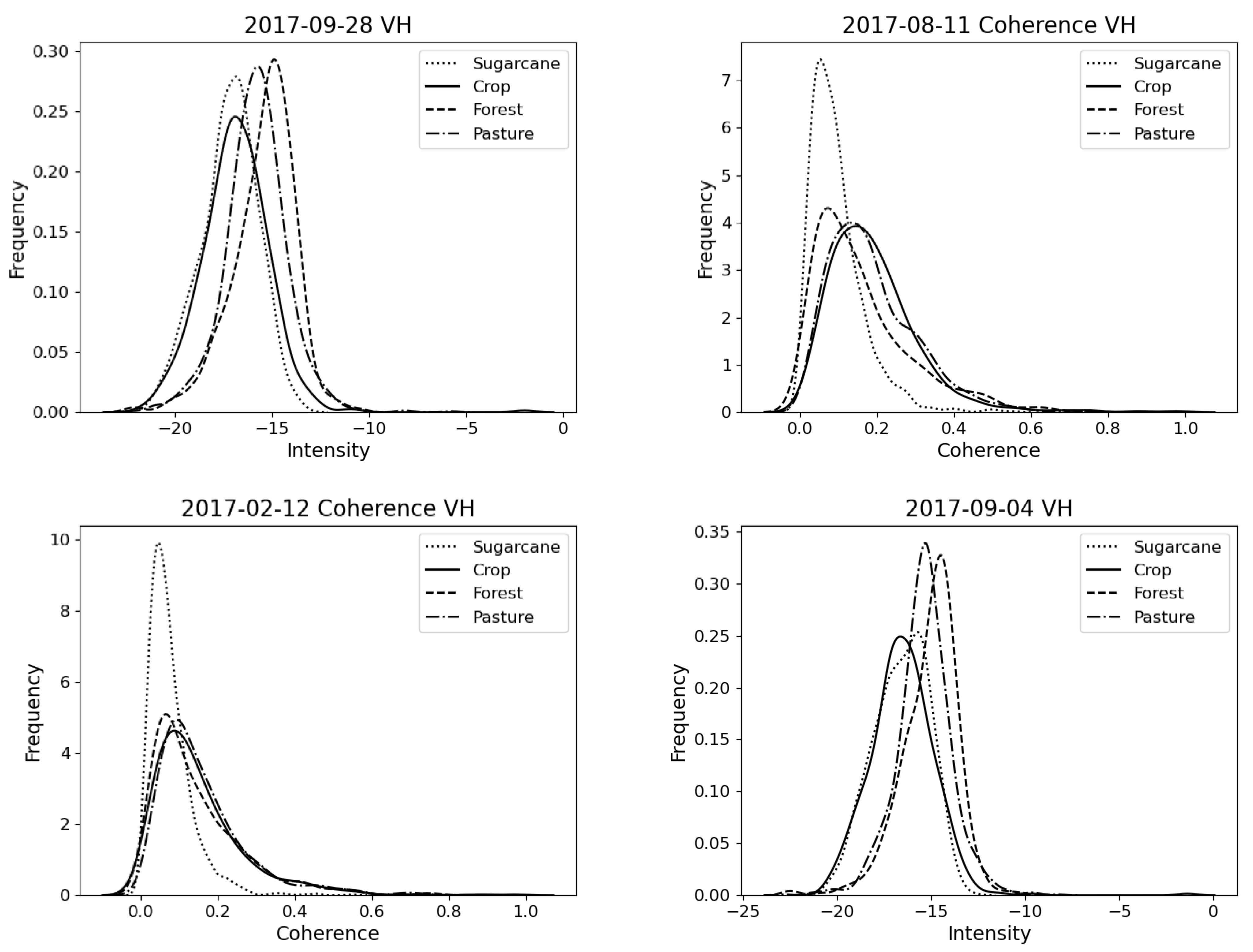
| Number | Date | Feature | Channel |
|---|---|---|---|
| 1 | 28 September 2017 | Amplitude | VH |
| 2 | 11 August 2017 | Coherence | VH |
| 3 | 12 February 2017 | Coherence | VH |
| 4 | 4 September 2017 | Amplitude | VH |
Publisher’s Note: MDPI stays neutral with regard to jurisdictional claims in published maps and institutional affiliations. |
© 2021 by the authors. Licensee MDPI, Basel, Switzerland. This article is an open access article distributed under the terms and conditions of the Creative Commons Attribution (CC BY) license (https://creativecommons.org/licenses/by/4.0/).
Share and Cite
Nikaein, T.; Iannini, L.; Molijn, R.A.; Lopez-Dekker, P. On the Value of Sentinel-1 InSAR Coherence Time-Series for Vegetation Classification. Remote Sens. 2021, 13, 3300. https://doi.org/10.3390/rs13163300
Nikaein T, Iannini L, Molijn RA, Lopez-Dekker P. On the Value of Sentinel-1 InSAR Coherence Time-Series for Vegetation Classification. Remote Sensing. 2021; 13(16):3300. https://doi.org/10.3390/rs13163300
Chicago/Turabian StyleNikaein, Tina, Lorenzo Iannini, Ramses A. Molijn, and Paco Lopez-Dekker. 2021. "On the Value of Sentinel-1 InSAR Coherence Time-Series for Vegetation Classification" Remote Sensing 13, no. 16: 3300. https://doi.org/10.3390/rs13163300