Abstract
Increasing woody cover and overgrazing in semi-arid ecosystems are known to be the major factors driving land degradation. This study focuses on mapping the distribution of the slangbos shrub (Seriphium plumosum) in a test region in the Free State Province of South Africa. The goal of this study is to monitor the slangbos encroachment on cultivated land by synergistically combining Synthetic Aperture Radar (SAR) (Sentinel-1) and optical (Sentinel-2) Earth observation information. Both optical and radar satellite data are sensitive to different vegetation properties and surface scattering or reflection mechanisms caused by the specific sensor characteristics. We used a supervised random forest classification to predict slangbos encroachment for each individual crop year between 2015 and 2020. Training data were derived based on expert knowledge and in situ information from the Department of Agriculture, Land Reform and Rural Development (DALRRD). We found that the Sentinel-1 VH (cross-polarization) and Sentinel-2 SAVI (Soil Adjusted Vegetation Index) time series information have the highest importance for the random forest classifier among all input parameters. The modelling results confirm the in situ observations that pastures are most affected by slangbos encroachment. The estimation of the model accuracy was accomplished via spatial cross-validation (SpCV) and resulted in a classification precision of around 80% for the slangbos class within each time step.
1. Introduction
Increasing woody cover and overgrazing in open semi-arid ecosystems are known to be one of the major factors driving land degradation [1]. In the context of this study, land degradation is defined as “the many human-caused processes that drive the decline or loss in biodiversity, ecosystem functions or ecosystem services in any terrestrial […] ecosystems” [2] (p. 28).
During recent decades, woody cover encroachment in open ecosystems has significantly increased in southern Africa, which have led to crucial environmental, land cover and land-use changes [3,4,5,6,7]. Venter et al. [8] concluded that the intensification of woody cover is not only connected to rising CO2 concentrations in the atmosphere, as a result of the human-induced global climate change, but it is also noticeable on regional aspects (e.g., extinction of large herbivore herds, and fires). However, CO2 fertilization improves water-use efficiency, due to the reduced stomatal conductance of woody plants [9]. Consequently, even with constant water ingestion, rising CO2 concentrations would lead to increased growth rates of woody biomass in relation to grass communities. Nevertheless, water availability and temperature are the key constraints on woody plant growth and are the crucial parameters in explaining encroachment patterns [5].
This study focuses on analyzing the spreading of the slangbos or bankrupt bush (Seriphium plumosum) in a selected test region in the Free State Province of South Africa. Though indigenous to South Africa, slangbos has been documented to be the main encroacher on the grassvelds (South African grassland biomes) in the provinces of the Free State, North West, Mpumalanga, Eastern Cape and Gauteng [10,11].
The rainfall optimum of Seriphium plumosum is between 620 and 750 mm per year [12], which lies between the semi-arid and mesic biome [13]. The shrub reaches a height and diameter of up to 0.6 m and has small light green leaves, which makes them perfectly adapted to long dry periods, compared to grass communities and the leaves are unpalatable to grazers due to their high oil content [14]. However, du Toit et al. [15] found that cattle graze young slangbos plants, which were regrown one year after active fire control measures. Slangbos prefers to grow on low fertile loamy soils, which makes hilltops and dry areas in the Free State vulnerable to this encroacher [16]. The encroachment of slangbos is responsible for a decrease in the grasslands productivity, pastures and livestock carrying capacity. The root system of Seriphium plumosum, which reaches a depth of up to 1.8 m and an extent of 1 m2 around the plant [14], competes with the surrounding grass for water and the availability of nutrients, which leads consequently to a reduction in the grass layer [17,18]. As slangbos is unpalatable for grazers, the shrub puts bigger pressure on the existing open grassland, which becomes vulnerable to overgrazing, increasing the potential of land degradation [16]. Moreover, slangbos is found to have high allelopathic potential, which impedes other plant species from finding suitable growing conditions in the surrounding area of a slangbos [19]. This poses great challenges to farmers on the one hand and for the local biosphere on the other hand. Approximately 11 million hectares of rangeland could become unsuitable for grazing if measures to eradicate the plant do not succeed. This could result in an annual loss of about ZAR 760,000 (South African Rand) (about EUR 44,000) for a 1000 ha livestock farm with a slangbos infestation of 50% of the pasture area [20].
Field observations detecting shrub distribution are cost intensive, time consuming and often do not address the spatial heterogeneity of encroachment patterns [21]. Earth Observation (EO) data from different sources and across different wavelengths (e.g., from ESA’s Copernicus Sentinel Programme) provide a suitable tool for mapping the extent and the velocity of woody encroachment [7,22,23,24,25]. The freely available optical and radar satellite data from the Copernicus Programme have short revisiting times (5 to 12 days) as well as high spatial resolution (10 m). Hence, they allow for monitoring woody cover encroachment in quasi near real-time and enable transferability and reproducibility in other regions. Bush encroachment mapping in southern Africa utilizing various sources of EO information (e.g., optical and radar) was investigated by recent studies [8,26,27,28,29,30,31]. These studies analyzed shrub cover increase, using high to low spatial resolution EO data investigating different approaches (e.g., land cover classification [27,31], random forest [8,26,29], trend analysis [28,30]). However, few studies have focused on one specific shrub species only. In general, an intensification of woody cover was present in all studies, especially in the open rangelands. Local studies revealed that protected areas with large herbivore populations (e.g., elephants) occasionally show a loss in woody or tree cover [27].
Remote sensing techniques are not likely to replace field measurements completely, as the validation of EO approaches deriving woody vegetation composition is still of high importance [21,32]. However, they allow for continuous wall-to-wall monitoring on a larger spatial extent of the parameter woody cover, which is considered an essential biodiversity variable [33].
The goal of this study is to monitor the slangbos encroachment on rangeland and pastures in the Free State Province, South Africa, between 2015 and 2020 by synergistically combining Synthetic Aperture Radar (SAR) (Sentinel-1) and optical (Sentinel-2) EO information. Both optical and radar satellite data are sensitive to the different vegetation properties and surface scattering or reflection mechanisms caused by the sensor specific characteristics. This study aims to (1) investigate the sensitivity of optical and radar remote sensing toward Seriphium plumosum and (2) to use combined SAR and optical dense time series to perform encroachment mapping on a regional scale in the South African grassland biomes. Utilizing time series, particular features in hyper-temporal radar and spectral data are examined to conclude the temporal variations observing Seriphium plumosum.
2. Materials and Methods
2.1. Study Area
The monitoring of slangbos encroachment was carried out on an approx. 90 km by 50 km (4500 km2) area located in the Free State Province between the towns of Ladybrand in the east and Botshabelo in the west (Figure 1).
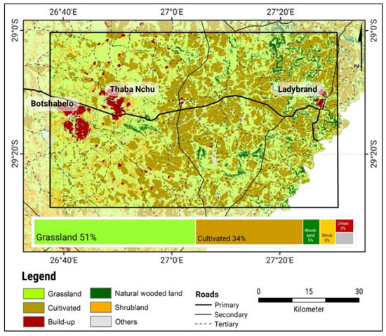
Figure 1.
The study area is located in the Free State Province, South Africa, close to the border of the Kingdom of Lesotho (in white). (Source: National Land Cover Classification of 2018 [34], Roads of South Africa [35]).
The region is part of the Highveld grassland ecosystem (1300 m–1700 m a.s.l.), which is characterized by a continental climate with a mean annual temperature of around 14 °C. However, days with temperatures below the freezing point are common during the winter season. The mean annual precipitation ranges from 500 mm to 700 mm, and the majority of rain occurs in the summer season between November and March [11].
The study area is known for extensive plains, cultivated areas and plateaus, which form the relief. The region is sparsely populated and mostly used for cattle and arable farming as well as water reservoirs. The primary land cover types are rangelands for grazing, cultivated land, shrubland and open grassland. The Highveld grassland biome is influenced by three major land degradation phenomena, namely (1) changes in plant composition, (2) loss of vegetation cover with a subsequent increase in wind and water erosion occurrence and (3) bush encroachment [11]. Moreover, the study area is one of the regions with the highest impact of invasive alien plant species throughout all of South Africa [36].
2.2. Data
2.2.1. Sentinel-1 and Sentinel-2
The Sentinel-1 and Sentinel-2 missions of the European Space Agency (ESA) Copernicus Programme have led to the increased availability of open access EO information covering both the optical and the microwave spectra. This opens new possibilities for the analysis of data with high spatial as well as temporal resolution for various applications, e.g., agricultural monitoring, and vegetation change analysis. The synergetic use of these EO data is especially valuable, as both satellites acquire data in parallel but measure different properties of the Earth’s surface. In comparison to Sentinel-2, Sentinel-1 acquires undisturbed images of the Earth’s surface, regardless of atmospheric effects and sun illumination.
For this study, Sentinel-1A C-Band SAR (5.405 GHz—approx. 5 cm wavelength) dual-polarized (VV–vertical/vertical, and VH–vertical/horizontal) scenes were utilized, covering the time period between 2015 and 2020 with a spatial resolution of up to 10 m. Sentinel-1 has a revisit time of a few days (3 to 12 days), depending on the geographic location and acquisition of both Sentinel-1A and -1B. In South Africa, the image acquisition repetition is twelve days [37]. In the Free State Province, only Sentinel-1A data from the ascending orbit are available, collecting images at around 5:00 p.m., local time. The Sentinel-1 footprint is represented by relative orbit numbers 14 and 116, which were used jointly.
The Sentinel-2 constellation consists of two satellites, namely Sentinel-2A (start of acquisition: November 2015) and Sentinel-2B (start of acquisition: August 2017). Since Sentinel-2B became operational, the revisit time has been approximately five days. In this study, data acquired between 2016 and 2020 from the optical Sentinel-2 constellation were used. Each of the two satellites (Sentinel-2A and -2B) has 13 bands covering the spectrum from the visible to the Short-Wave-Infrared (SWIR) and a maximum spatial resolution of 10 m. The images are acquired at around 10:30 a.m. local time [38].
In this study, Sentinel-1 Single Look Complex (SLC) and Ground Range Detection (GRD) images were utilized. Whereas the SLC data comprise the phase information, which is used to derive the interferometric coherence, the GRD data contain only the amplitude and are already multilooked. In total, 313 Sentinel-1 GRD, 145 Sentinel-1 SLC (144 coherence pairs) as well as 503 Sentinel-2 images were utilized. For the coherence estimation, Sentinel-1 SLC scenes from the relative orbit 14 were used.
2.2.2. Agricultural Statistics 2014–2018
Spatial information for the different crop types planted in the study area was provided by the Department of Agriculture, Land Reform and Rural Development (DALRRD) [39]. The dataset contains information of crop types planted between 2014 and 2018, where each dataset represents an individual crop year. A crop year is defined from June until May of the next year, and includes both winter (June–September) and summer (October–May) planting seasons.
In general, the Free State Province has the highest number of farming units, which are summed up to almost 8000 entities, which represent approximately 20% of the national total. Approximately 460,000 km2 are used for agriculture of which 80% were used for grazing and the remaining 20% were used mainly for dryland crop production [40].
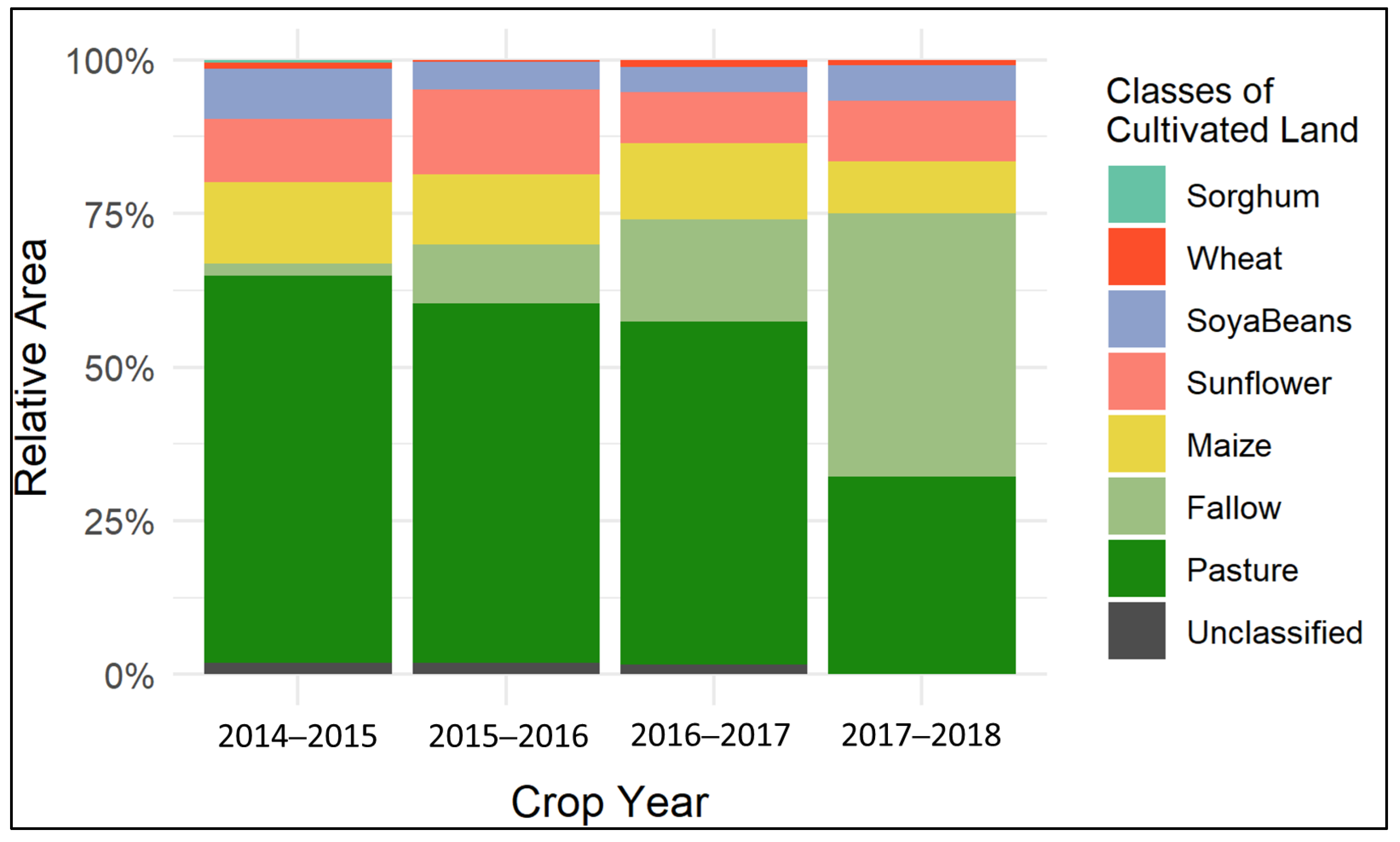
Between 2014 and 2018, the cultivated land in the study area was dominated by pasture vegetation (Figure 2). Maize, sunflower and soybeans can be identified as major crops during the same period, whereas the amount of wheat and sorghum is negligible. However, fallow land areas, which are certainly prone to a slangbos invasion, have shown a significant increase between 2014 and 2018, with the largest expansion between 2016/17 and 2017/18.
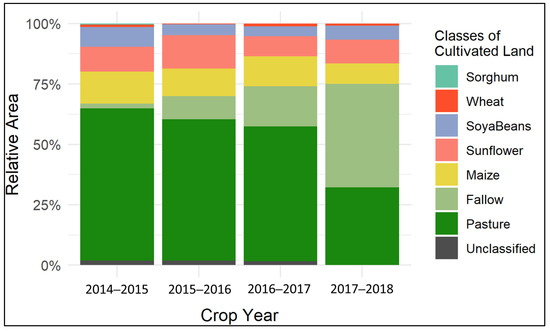
Figure 2.
Area for different cover types of the cultivated land within the study area for the crop years between 2014 and 2018 (Source: [39]).
In 2014/15, croplands (approx. 380 km2 (33%)) and pasture (approx. 730 km2 (63%)) covered most of the cultivated land within the study area. At this time, the study region was characterized by 23 km2 (2%) fallow land. In 2015/16, the area covered by fallow land increased by 7% to an area of 110 km2, where both, pasture and cropland declined by equal percentages. Soybeans showed the largest decline during that time, which was followed by a slightly increasing trend toward 2018. In 2016/17, the statistics show that especially cropland turned into fallow land, which increased by approximately 7% to an area of 190 km2. Sunflower showed the largest decline during that period (60 km2 (5%)). In 2017/18, the class fallow showed the largest increase to 43%, which equals around 480 km2. At this time, the area, which was covered with pasture beforehand, decreased by about 280 km2 (23%), whereas the number of croplands had no significant loss. However, a large decline for maize was found in this year (50 km2 (4%)), as these areas were changed to soybeans or sunflowers.
2.2.3. Reference Data
The essential ground reference sites were exploited via field exploration, aerial photo documentation and local expert knowledge. In order to scale the amount of ground validation, the Google Earth high-resolution time series imagery [41] and the National Geo-spatial Information (NGI) very high resolution aerial photos [42] were used. The previously identified slangbos sites were used as a blueprint for creating a set of labeled fields in the area, utilizing manual mapping in cooperation with local partners at DALRRD [39]. The ground references consist of binary spatial polygons indicating the occurrence or absence of slangbos. An oversampling of the critical slangbos and grassland land cover was performed to draw the focus of the classification algorithm to this discrimination task. Finally, the labeled dataset totals up to roughly 14 km2, which makes up 1.2% of the agricultural area and 0.3% of the entire study area.
2.3. Methods
2.3.1. Sentinel-1 Pre-Processing
The Sentinel-1 GRD data were pre-processed using PyroSAR [43], which is designed for large-scale SAR satellite data processing within a Python framework. It offers a complete solution for organizing and processing SAR data for different historical and current satellite missions, with additional functionalities, which are available after the pre-processing of the SAR satellite images (e.g., mosaicking and resampling images to common pixel boundaries suited for time series analysis). PyroSAR offers the possibility to utilize the open-source ESA’s Sentinel Application Platform (SNAP) as well as the GAMMA Remote Sensing software for licensed users.
The Sentinel-1 GRD data were pre-processed using GAMMA (Software Version: July 2018, GAMMA Remote Sensing AG, 3073 Gümligen, Switzerland) [44]. (1) To convert from digital numbers (DNs), which are recorded by the sensor, to physical units, a radiometric calibration was applied for each dataset. (2) The orthorectification of the data was carried out, using the precise orbit state vectors (precise orbit ephemerides, POE) as well as height information from the Shuttle Radar Topography Mission (SRTM) Digital Elevation Model (DEM) [45] at 30 m spatial resolution. (3) The conversion of beta naught (β0) to gamma naught (γ0) values was achieved by a terrain flattening [46], utilizing the SRTM DEM.
The interferometric coherence (γ) represents a measure of the correlation between two complex SAR images and can be described as follows:
where u1 and u2 are two complex (SLC) acquisitions, |u1| and |u2| are their amplitudes, and E[x] is the expected value of the considered variable x. The coherence takes values between 0 and 1, where 0 represents no correlation and 1 represents a perfect correlation between the image phases [47,48]. Depending on the backscattering properties of the surfaces and their variation over time, the coherence is variable; therefore, it is useful for land cover classification [49,50], and biomass estimation [51,52], as well as for change detection (e.g., mapping deforestation) [53,54].
The Sentinel-1 SLC data were pre-processed, using SNAP. The coherences were only calculated for the co-polarized mode (VV) because of the stronger signal and thus higher signal-to-noise ratio. The coherence estimates were created for all adjacent date pairs with a temporal baseline of 12 days. However, in 2015 and 2016, eight interferometric coherence pairs (four in each year) were based on a 24-day temporal baseline, which was caused by the interruption in the acquisitions due to maintenance or other technical related issues at the early lifetime of the satellite.
(1) The first processing step was to apply the orbit state vector files to the SLC data, using the precise orbit state vectors (precise orbit ephemerides, POE). (2) As the SLC images are acquired in three sub-swaths (one image per swath and polarization) in TOPSAR mode (Terrain Observation with Progressive Scans SAR), the TOPSAR split function was applied to calculate the coherence based on each sub-swath. (3) In order to co-register the SLC swaths of an image pair, the back-geocoding function was accomplished utilizing the height information from the SRTM DEM [45] at 30 m spatial resolution. (4) The coherence between both SLC datasets was calculated using the interferogram module in SNAP. (5) TopSAR merge was utilized to merge the individual sub-swath before performing (6) the terrain correction, which also utilized the SRTM DEM dataset as the height information.
2.3.2. Sentinel-2 Pre-Processing
Sentinel-2 L1C products consist of TOA (top of atmosphere) reflectances in cartographic geometry. The Sentinel-2 data are provided in tiles with a fixed coverage of about 10,000 km2 (100 by 100 km) projected in UTM/WGS84 along a single orbit [38].
In order to obtain the bottom of atmosphere reflectance, the Sen2Cor processor [55] was utilized with additional parameter settings, such as aerosol optical thickness and water vapor, but without the correction for cirrus and terrain. Each band of the pre-processed Sentinel-2 L2A products has the identical spatial resolution as the original L1C input band, namely 10 m for bands 2, 3, 4, 8, 20 m for bands 5, 6, 7, 8a, 11, 12 and 60 m for bands 1, 9, 10. In addition, the Python application [56] of the FMask algorithm [57,58,59] was used to produce cloud masks with a resolution of 20 m from the Sentinel-2 L1C data.
To assess the sensitivity of the satellite image data concerning vegetation processes, the NDVI (Normalized Difference Vegetation Index) [60] and SAVI (Soil Adjusted Vegetation Index) [61] were retrieved from each Sentinel-2 L2A scene with a spatial resolution of 10 m:
where N corresponds to the near-infrared (NIR) channel of Sentinel-2 (band 8), R corresponds to the red channel of Sentinel-2 (band 4) and L is a factor, which is used to minimize the influence of the soil brightness in the SAVI (here L = 0.5) [61].
Vegetation dynamics for a specific area are often analyzed using time series constructed from indices. Here, time series were constructed with the entire Sentinel-2 data archive from 2016 to 2020. To avoid spurious data due to atmospheric distortions, each index file was masked with the corresponding FMask product before stacking. In some regions, depending on the weather conditions in combination with the topography, each time series along a pixel stack can have substantial gaps lasting up to eight weeks. However, with the introduction of Sentinel-2B, gaps in areas with intensive cloud cover are considerably shorter, with at least one suitable acquisition each month.
2.3.3. Combined Time Series Analysis
For enhancing the interpretability of the dense time series, we employed the smoothing algorithm, Friedman’s “super smoother” [62], an adaptive, variable-span linear smoother. It provides a smoothing prediction due to the adaptive spans and utilization of the parameter of least residuals. The default setting provided in the R-implementation was found to be the most suitable for the interpretation of the time series.
2.3.4. Predictive Modeling and Interpretation
In order to predict the spatial distribution of slangbos on cultivated land, a random forest model was fitted for each crop year and validated using spatial cross-validation (SpCV) [63]. Random forest models are widely used in remote sensing applications due to their robustness to overfitting and flexible approach to recognizing non-linear structures in feature spaces [64,65].
In this study, the predictor set consists of optical indices from Sentinel-2 (NDVI, SAVI), co-polarized (VV) and cross-polarized (VH) Sentinel-1 backscatter as well as coherences (VV) comprises 67, 154 and 119 features for each investigated crop year 2015/16, 2016/17 and 2017/18, respectively. The model was trained on a labeled set of 5000 randomly selected pixels, indicating slangbos and non-slangbos fields. Due to the anticipated spatial autocorrelation effects, the model was cross-validated with 100 iterations and 5 folds of k-nearest-neighbor spatially segmented test data sets in order to derive accuracte metrics of the model predictions presented.
The random forest models were assessed, using the overall accuracy (OA) throughout all model runs. The OA includes the model performance on both slangbos and non-slangbos sites and is, therefore, prone to an overoptimistic classification performance. Therefore, the averages of recall (how much slangbos were missed) and precision (how much slangbos were falsely assigned) were also estimated in order to assess the capacity of the model to distinguish slangbos. An independent validation approach, utilizing in-situ data, which are not part of the machine learning methodology, was not applicable, as no such additional ground data were available. Hence, this study relies on the results of the internal spatial cross-validation of the random forest approach, which is a feasible approach and was utilized by other studies to reduce the overoptimistic model performance when using only random distributed points instead of spatially separated folds [66].
Since the hyperparameter settings for random forests are relatively stable [67,68,69], no separate tuning was set up. The number of trees ntrees was set to 300 (large and stable averaging possible) with mtry = √P, where P is the number of features in the model [70]. These parameters were optimized prior to model fitting, as they were found to be sensitive with respect to model accuracy and computation time. The so-called model tuning was carried out to identify the best parameter set for the SpCV and training [71,72]. Other parameter settings were left as the default.
The random forest feature importance determines how much each feature decreases the impurity weight when kept out of the model. It was proven to be a reliable means of assessing feature importance on the model predictions while accounting for all other predictors in the model [73]. It must be mentioned that correlated predictors take away their ranks as features akin to compensate for the loss of information. The model setup, the retrieval of feature importance and the SpCV are implemented in the R software package mlr3 [74] with bindings to sperrorrest [63].
3. Results
3.1. Combined Time Series Analysis of Sentinel-1 Backscatter and Coherence and Sentinel-2 NDVI and SAVI
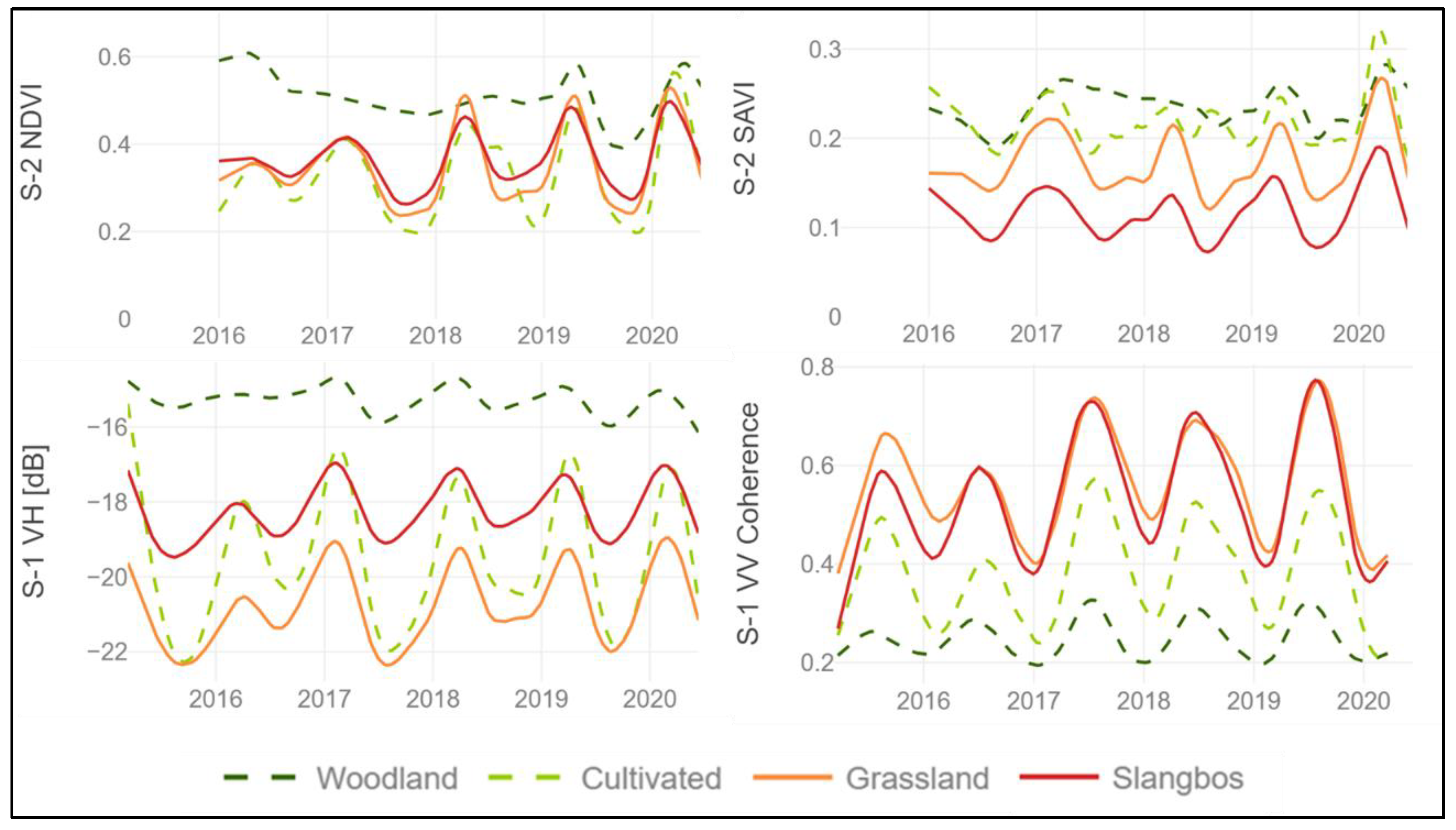
The input variables for the random forest approach classifying the spreading of slangbos in the study area were (1) the Sentinel-1 backscatter (S1 VV and S1 VH), (2) Sentinel-1 coherence (S1 VV), (3) Sentinel-2 NDVI and SAVI time series. This section highlights the temporal profiles of these variables for different land cover classes (slangbos, grassland, woodland and cultivated areas) (Figure 3) in order to investigate which parameter could be best suited to distinguish between the slangbos class and the other classes. In addition, precipitation information from the CHIRPS (Climate Hazards Group Infrared Precipitation with Stations) product [75], which represents rainfall estimates from rain gauge and satellite observations, was utilized to account for the characteristics of the dry and wet season to the time series signal.
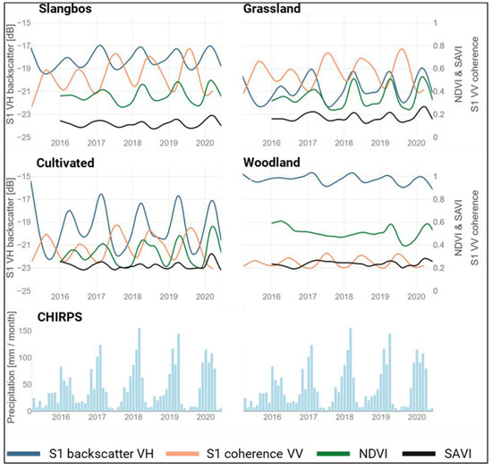
Figure 3.
Temporal dynamics of the Sentinel-1 VH backscatter, Sentinel-1 VV coherence, Sentinel-2 NDVI and SAVI time series. In addition, precipitation information from the CHIRPS (Climate Hazards group Infrared Precipitation with Stations) product [75].
Areas with slangbos encroachment are characterized by a clear increasing trend of the cross-polarized VH backscatter intensities. This is especially true between 2016 and 2017. Afterwards it seems to be stabilized, as it is also noticeable for the other classes cultivated and grassland. At the beginning of the time series, the severe drought of 2015/2016, which had a vast impact on the vegetation development during these years [76,77,78], is clearly visible. The sparse precipitation indicated in the CHIRPS product in 2016 can be seen as an additional indicator of the drought. InSAR coherences similarly show low amplitudes in the first two years of the time series. Yet, this trend fades in years that were not drought-affected. Therefore, the drought may have affected a stronger slangbos growth. The coherence only shows increase and stabilization, compared to the other culture types where the coherence decreases between 2015 and 2016 and then increases afterwards. The SAVI time series is characterized by low amplitudes mainly in ranges between 0.1 and 0.2, while NDVI ranges between 0.2 and 0.6 at high amplitudes. During the drought, the amplitude of either optical index was lower. In comparison, the NDVI has higher values as well as higher amplitudes during the entire time series when compared to the SAVI.
Grasslands exhibit lower cross-polarized VH backscatter values, compared to the slangbos areas. These circumstances are due to the higher proportion of volumetric scattering effects in the slangbos shrubs compared to the vertically oriented grasses. However, the impact of the drought is also visible at the beginning of the time series. Thus, dry grasslands or grasslands fallen barren due to water scarcity result in reduced backscatter. The amplitude of the coherence is similar during the entire period when compared to slangbos but shows larger dynamics when related to the other classes. The SAVI indicates slightly higher temporal dynamics in comparison to areas infected by slangbos growth during the entire time series.
The woodland areas reveal higher backscatter values, compared to the other classes, which is a result of the volumetric scattering mechanism in the crones of upper tree canopies. The amplitude of the cross-polarized backscatter is low, which reflects almost no seasonality in the woodland areas. The temporal profile of the coherence is quite low (decorrelation) with also low seasonality.
The cultivated areas show the largest Sentinel-1 VH backscatter dynamics, which is caused by the harvest cycles. This is also true for the NDVI signal. The SAVI is somewhat comparable to the grassland class, with lower seasonal dynamics. The impact of the severe drought in 2015/2016 is visible between 2016 and 2017, which could be identified as repercussions of the drought to the vegetation growth.
The comparison of the temporal signature of the four different parameters for the classes slangbos, grassland, woodland and cultivated areas, have indicated that the Sentinel-2 derived SAVI index, as well as the Sentinel-1 VH backscatter, shows the highest potential in separating between the class slangbos from the others. Figure 4 shows the comparison between the NDVI and the SAVI as well as Sentinel-1 VH backscatter and VV coherence for the four classes. While the NDVI confirms no separability between slangbos, grasslands and cultivated areas, the SAVI provides a more potent means of discriminating these classes. In addition, the Sentinel-1 VH backscatter time series for slangbos delineate from the other classes when compared to the Sentinel-1 VV coherence.
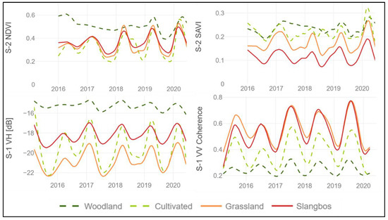
Figure 4.
Separability of the class slangbos from other land cover classes for the variables Sentinel-1 VH backscatter, Sentinel-1 VV coherence, Sentinel-2 NDVI and SAVI time series.
3.2. Classifying Slangbos using Random Forest
3.2.1. Variable Importance
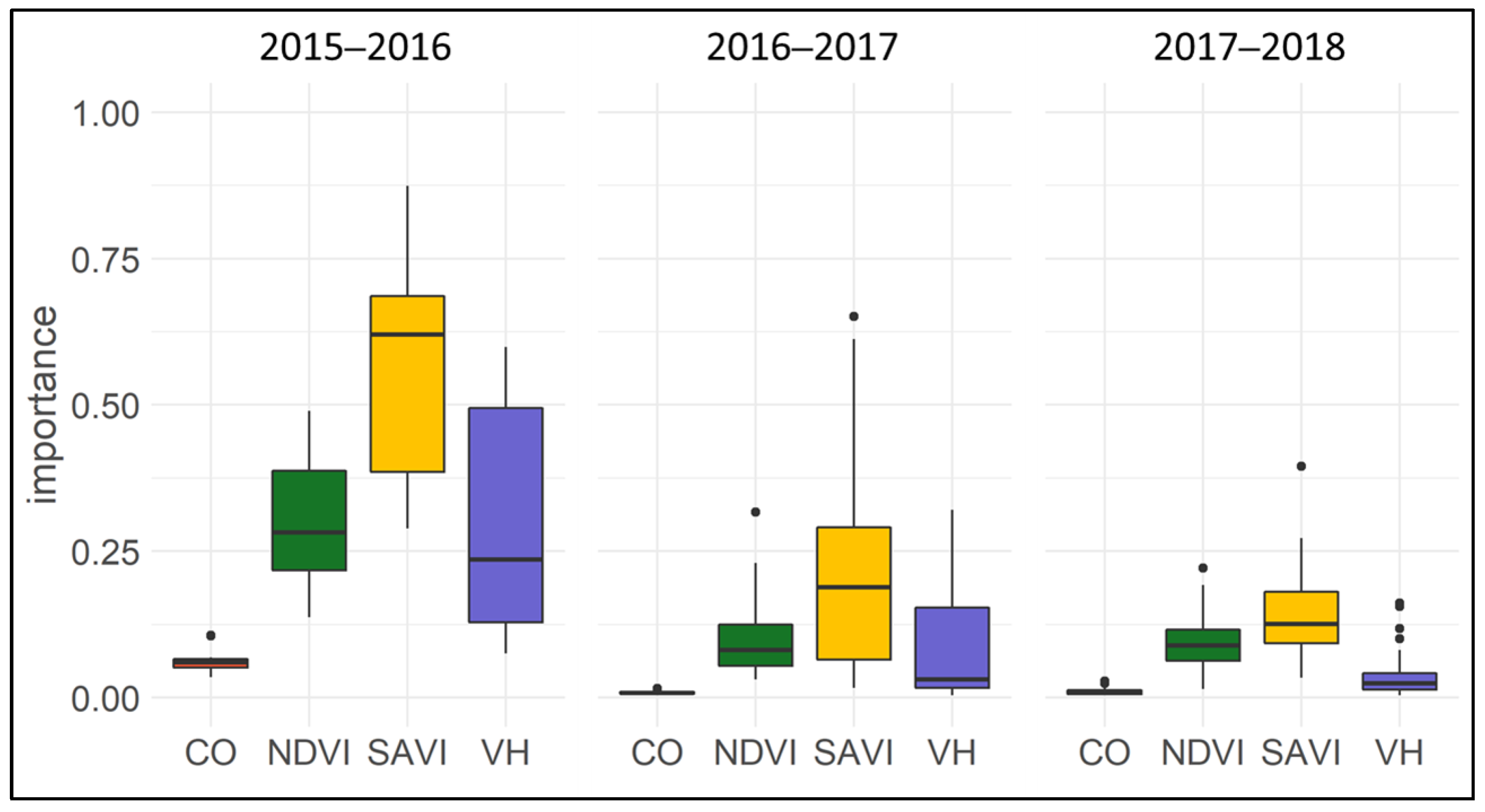
The variable importance was calculated for the crop years between 2015 and 2018 (Figure 5). The results show that the Sentinel-2 derived SAVI has the highest importance for the classification algorithm (refer to Section 3.2, Figure 4). This is especially true for the crop years 2015 to 2016. However, this year needs to be analyzed with caution, as the Sentinel-2 data are only available from early 2016, and thus are not available for the entire crop year. During the same crop year, the NDVI, as well as the cross-polarized Sentinel-1 VH data, have important contributions to the classification result. The Sentinel-1 VV coherence results in the lowest variable importance for all observed crop years. During 2016 and 2018, the variable Sentinel-1 VH had less significance for the classification algorithm when compared to the Sentinel-2 derived NDVI. This importance must be handled with care, as a higher abundance of a feature subset, e.g., the denser time series of Sentinel-1 compared to cloud-free Sentinel-2 acquisitions result in a relatively lower overall importance of that feature subset. However, the optical indices and cross-polarized SAR still dominate the bulk of the model performance. The inter-comparison between the years is further dominated by the number of predictors used for modeling, e.g., the crop year 2017/2018 shows the lowest importance, as the highest number of predictors was used.

Figure 5.
Variable importance for the input parameters Sentinel-1 VV coherence (CO), cross-polarized Sentinel-1 backscatter (VH) as well as Sentinel-2 derived NDVI and SAVI.
3.2.2. Spatial Cross-Validation (SpCV)
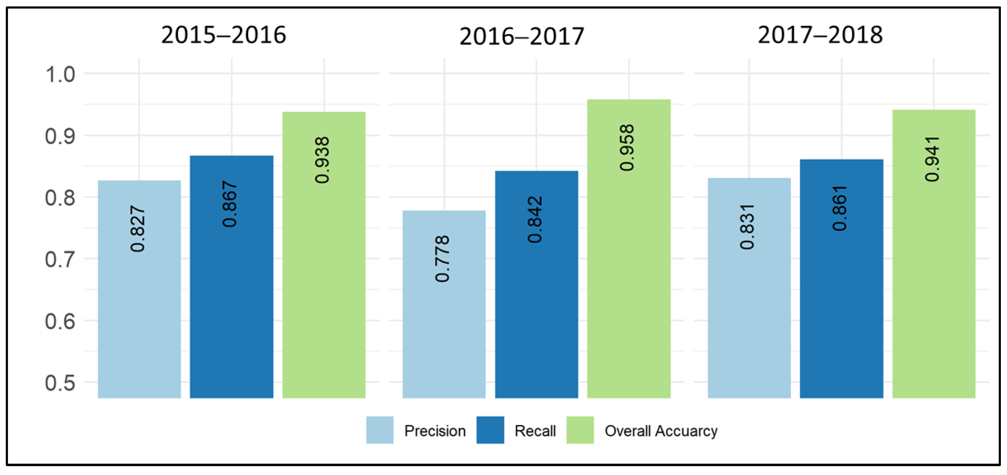
The spatial cross-validation was carried out for each of the crop years between 2015 and 2018. Figure 6 shows the accuracies of the binary classification of the categories slangbos as well as non-slangbos. The overall accuracy exceeded 90% for the entire period. The precision measure indicates to what extent the slangbos was correctly classified (around 80%). The recall measure is even higher, which is an indicator of how much slangbos was missed during classification (13% to 16%). Slightly lower precisions were found for the years 2016/17 and 2017/18.
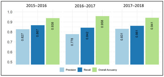
Figure 6.
Classification accuracy metrics derived from spatial cross-validation for each of the crop years between 2015 and 2018.
3.2.3. Slangbos Probability Measures
The probability measure is an output of the random forest algorithm and describes the potential assignment of the individual pixel to the class slangbos between 2017 and 2018 [79] (Figure 7, left).
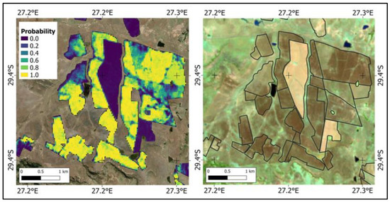
Figure 7.
An example of the probability measure mapping slangbos encroachment in the project area. The comparison with an optical image illustrates how the probability index reflects the heterogeneity within fields. Left: probability measure for the assignment of individual pixels to the class slangbos between 2017 and 2018. Right: Sentinel-2 Short-Wave Infrared (SWIR) image from 30.08.2017 (RGB = bands 12-8A-4). (Field boundaries source: [39]; contains modified Copernicus Sentinel data [2017–2018]).
The figure gives a detailed insight into the different characteristics of agricultural fields being potentially infected by slangbos growth. The dark field in the center of the image is surrounded by fields with high probabilities for slangbos encroachment, which is also visible as brownish areas in the optical Sentinel-2 image (Figure 7, right). In combination with the Sentinel-2 images, it can be illustrated how the probability index reflects the heterogeneity within each of the fields. This information might be utilized to identify areas that need to be prioritized for slangbos-clearing investigations within a slangbos encroachment monitoring system.
3.3. Mapping
3.3.1. Regional Scale Analysis
Figure 8 shows the distribution of the areas which were identified to be infected by slangbos encroachment for the entire study area between 2015 and 2020. The presented areas were not used for model training. Areas in red are dominant and relatively homogeneously distributed in the entire study area. These areas indicate that slangbos were prevalent during the beginning of the time series in 2015/2016. Blue areas are spread between the southern and the eastern part of the study area. The patches indicate slangbos and shrub cover during the second half of the time series, after 2017. These areas are likely to be those that were infected by the growth of slangbos or shrub encroachment during that time period. Few areas are classified as green, which indicate slangbos only found in 2017, which are often adjacent to orange areas, indicating slangbos or shrub cover also in 2015. These regions might be areas in which slangbos and shrub cover were cleared either by hand or due to fires.
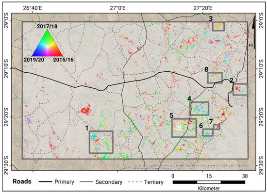
Figure 8.
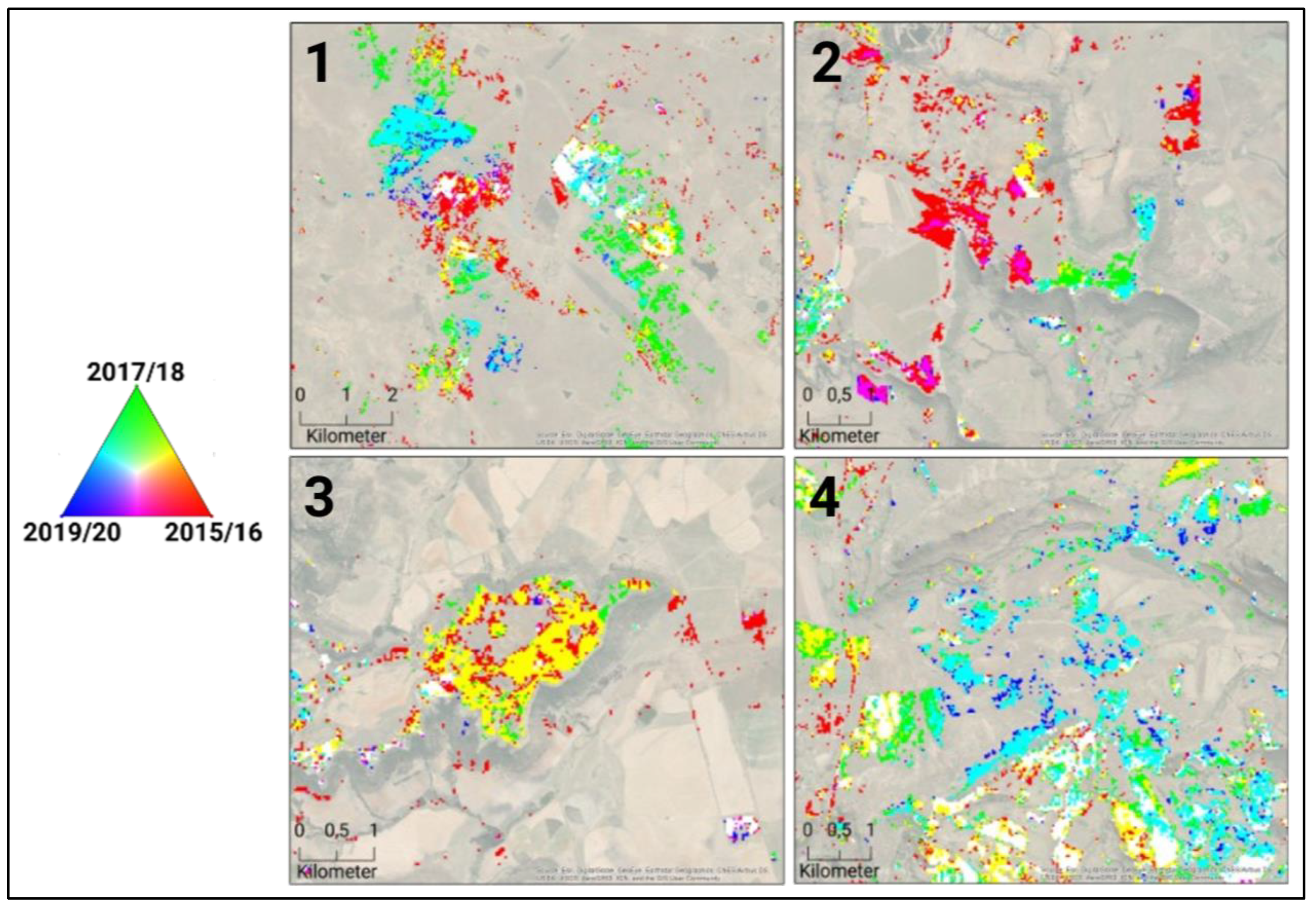
Spatial distribution of the regions affected by slangbos encroachment for the entire study area between 2015 and 2020. This map represents each crop year in a specific layer of the RGB composite (R: 2015/16, G: 2017/18, B: 2019/20). The numbered boxes show the zoom-in for a detailed analysis within the next sections. (Roads: [35], Map data source: Esri, DigitalGlobe, GeoEye, Earthstar Geographics, CNES/Airbus DS, USDA, USGS, AeroGRID, IGN, and the GIS User Community).
Figure 9 highlights four areas, showing the classification result within the rangeland areas to describe the spatial pattern in more detail. Area 1 is a heavily encroached prone site. The local partners from LandCare confirmed this site to be cleared during our observation period. In particular, the red areas in the rangelands were cleared between 2015 and 2019. On the other hand, regrowth in recent (since 2017) years is found in other areas, which are shown in cyan. In the center, some white areas are visible, indicating slangbos infection during the entire period. In Area 2, a fire occurred in September 2017, which resulted in a massive loss of shrub cover (green areas) [80]. On the other side, shrub encroachment on native rangelands is found on the eastern part of the plateau (red areas). Area 3 is a large managed site, where also shrub clearing took place during the second half of the observed period. Area 4 is characterized by intensive shrub encroachment in the rangeland sites since 2017/2018. The classification algorithm was able to even detect these small areas.
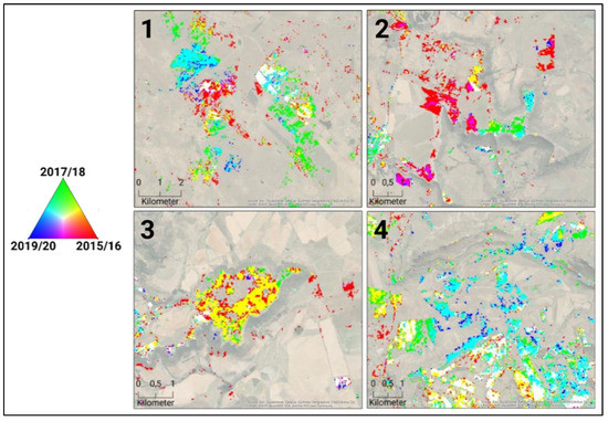
Figure 9.
Subset of the boxes 1 to 4 (Figure 8) showing slangbos infected areas in the rangelands (R: 2015/16, G: 2017/18, B: 2019/20). (Map data source: Esri, DigitalGlobe, GeoEye, Earthstar Geographics, CNES/Airbus DS, USDA, USGS, AeroGRID, IGN, and the GIS User Community).
3.3.2. Field Boundary Scale Analysis
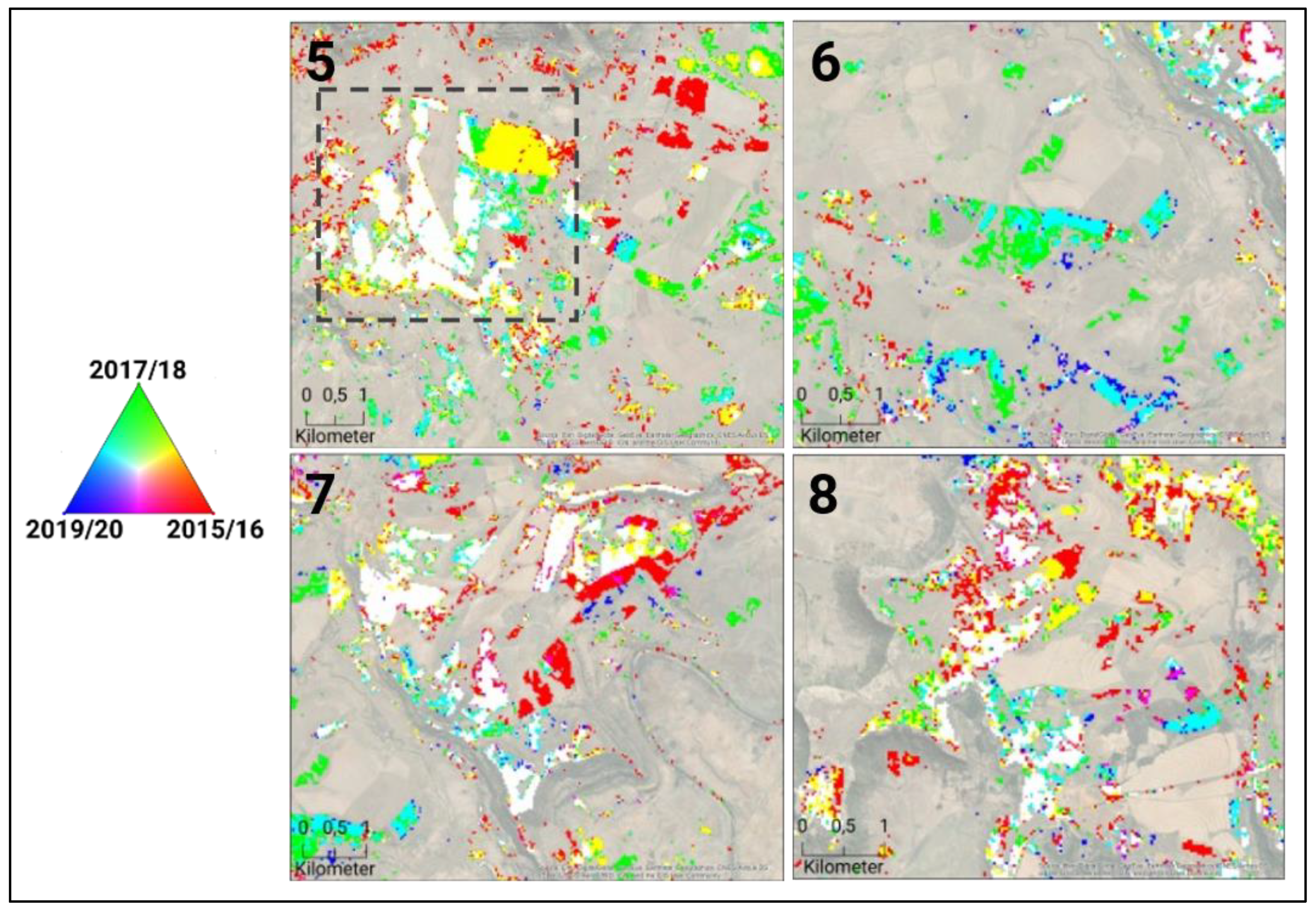
Figure 10 highlights four areas within the cropland boundaries, which were provided by the DALRRD [39]. The region inside the grey dashed line in area 5 is identical to the subset shown in Figure 7, which was utilized to show the classification results of the model. This region shows heavily encroached pastures, where some of them were found to be fallow. Large areas are shown in white, indicating that slangbos were growing on the rangelands during the entire time period. Area 6 illustrates areas that were rapidly encroached by slangbos in 2017/2018 (turquoise and blue). Green areas are likely caused due to misclassifications, as it would mean that slangbos only occurred in 2017/18 and suddenly disappeared. However, man-made clearing management or fires might also be causing this spatial pattern. Area 7 represents a vast shrub control side, where large areas were infected by slangbos during the entire time (white areas); some areas show the effect of clearing actions after 2015/16 (red areas). Area 8 shows a diverse spatial of different slangbos encroachment dynamics. Some areas indicate slangbos infections during the entire period. Large areas show slangbos clearing activities, which are shown in red (cleared in 2015/16) and yellow (cleared after 2017/18). Small areas indicate slangbos infections during the later stage of the time period (turquoise), which might be fields, which were cleared a few years before and when already affected by slangbos encroachment.

Figure 10.
Subset of the boxes 5 to 8 (Figure 8) showing slangbos infected areas in the field boundaries by crop years (R: 2015/16, G: 2017/18, B: 2019/20). The grey dashed line in subset 5 represents the region shown in Figure 7. (Map data source: Esri, DigitalGlobe, GeoEye, Earthstar Geographics, CNES/Airbus DS, USDA, USGS, AeroGRID, IGN, and the GIS User Community).
The crop statistics were used to identify which crop type classes are affected the most by the encroachment of slangbos. Figure 11 indicates the relative area covered by slangbos on cropland, fallow land and pastures between 2015 and 2018. It needs to be mentioned that only time period for which crop statistics were available is covered. Thus, recent years were not accessible through the DALRRD, as these data were still classified for internal use only at the time of writing.
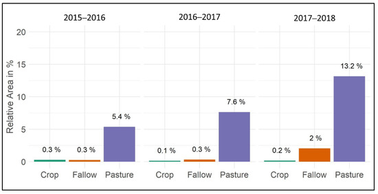
Figure 11.
Relative area (in %) statistics on slangbos encroachment of different agricultural land types (cropland, fallow land and pastures).
The statistics on slangbos encroachment of different agricultural land types clearly demonstrate that pasture areas are highly affected by the encroachment of slangbos. Fallow areas also show some sensitivity to infection by the growth of slangbos. Croplands reveal almost no sign of being affected by the encroachment of slangbos, which is attributed to intensive management (i.e., plowing) throughout harvest cycles. These findings are an indication for the reliabilty of the classification approach, as we did not expect slangbos encroachment on croplands, due to the intensive management.
4. Discussion
This study focused on the classification of slangbos encroachment on agricultural land, using ESAs Copernicus Sentinel-1 and Sentinel-2 time series between 2015 and 2020 for a test area in the Free State Province, South Africa. The classification accuracies of over 80% indicate a solid approach for slangbos encroachment mapping, using optical and radar time series information from ESAs Sentinels data. Moreover, the random forest classifier was used as a framework for the multi-temporal and multi-sensor classification.
The paper investigated slangbos encroachment on a comparatively small study area of around 4500 km2, where slangbos is known to be the main encroacher. The agricultural statistics revealed that fallow areas increased dramatically after 2015 and doubled until the end of 2018. In this year, fallow areas covered more than 50%, with the remaining areas being almost evenly distributed amongst croplands and pastures. This abandonment of agricultural land is a known phenomenon of the land-use change in South Africa, which is driven by climate as well as socio-economic factors [81]. The statistics on slangbos encroachment of different agricultural land types revealed that this process is more recent in abandoned crop areas as compared to regions near settlements [82].
Upcoming research activities might focus on larger areas, where other bush communities or shrub types represent the main invader. As an example, it is worth mentioning the black wattle (Acacia mearnsii), which also imposes great pressure on grassland communities in South Africa [83,84]. Hence, future studies could build upon this methodology to aim for the discrimination between different shrub communities in regions, where a mixture of different encroachers is present. If the goal is to classify different shrub communities, the presented binary approach has limitations in the separation of different encroachers. This might need additional data (e.g., hyperspectral [85]) for the training of more suitable machine-learning models.
However, classifying different shrub communities is likely to introduce other issues, such as spectral and scattering uncertainties, which can be attributed to the canopy spacing of the individual plants that need to be considered in future studies. Depending on the spatial resolution of the data, the influence of grass and soil between shrubs need to be analyzed in more detail, as it has major impacts on the reflectance and backscatter. Further research will increase the knowledge of those scattering mechanisms of slangbos and other bush communities in contrast to grassland. Regarding the classification of slangbos, it is likely that the Sentinel-2 derived SAVI as well as the Sentinel-1 VH backscatter are of higher potential than the NDVI and Sentinel-1 VV coherence. In the case of the SAVI, it might be attributed to the fact that slangbos patches grow more sparsely, and thus benefit from the bare soil consideration in the SAVI estimation, as the influence of the soil brightness is reduced in comparison to the NDVI [86]. As droughts might favor bush encroachment [87,88], it is of high importance to integrate information on precipitation dynamics in future studies. Here, we utilized coarse resolution CHIRPS data for analysing the yearly precipitation dynamics. Since rainfall events might occur locally, information from climate stations or data products with higher spatial resolution could be of great value for upcoming investigations.
To make the model performance more flexible and effective as well as applicable for investigations in other or larger regions, the training input should be limited to only important model features. In this study, more than 500 features were used as model training input, with around 100 for each individual crop year. These might be not applicable when transferring the methodology to other larger regions. To enhance the model performance and based on the known variable importance, Sentinel-1 VH backscatter, Sentinel-2 SAVI and NDVI time series might solely be utilized as input variables. Methods for interpretable machine learning and feature selection are desirable for future research, making the models comprehensible and transparent. In addition, the use of statistical metrics from hyper-temporal EO data might be a feasible solution to analyze time series in a cost-effective and descriptive way. Simple descriptive statistics, such as median, standard deviation or quantiles in conjunction with regression functions or temporal filters might improve the model performance as well as classification results.
The availability of agricultural statistics for the entire observation period is crucial for the identification of classes that were infected by slangbos encroachment. In this study, the statistics were available between 2014 and 2018 only. Hence, statistics for two crop years (2019 and 2020) were missing.
Future investigation might utilize different measures to assess the accuracy. In this study, we measured the accuracies based on a binary classification (slangbos and non-slangbos), which integrates issues related to the sample size of both classes. The overall accuracy might be not reliably interpretable in this case, whereas recall and precision are more valuable measures. The overall accuracy is prone to the imbalance of the sample size between the slangbos and non-slangbos classes [89]. The recall marks the rate of “missed” slangbos pixels, while the precision is the rate of falsely detected slangbos areas. Both numbers can be low, as they are only based on true positive, false negative and false positive values. The true negative sample size is extremely large, as is common in most remote sensing classifications since they include all classes, e.g., water, urban, and grassland, pixels.Upcoming investigations should emphasize the potential of mapping slangbos encroachment, using cloud-based solutions (e.g., Google Earth Engine) to minimize the data processing times for the users. This might result in a bush encroachment monitoring system, where products are directly accessible by the users without any data interaction. Such a monitoring system is likely to result in an early warning system using near-real-time classification approaches, advances in the potential of current methodologies identifying infected areas, as well as helping to plan optimal clearing strategies supporting sustainable land management strategies.
5. Conclusions
The objective of this paper was to monitor slangbos encroachment between 2015 and 2020 in a test region in the Free State Province, South Africa. The slangbos classification was carried out utilizing a synergetic combination of Sentinel-1 and Sentinel-2 time series within a machine-learning framework, applying a random forest classifier. Field inventory and high-resolution image analyses as well as spatial crop statistics and slangbos verified areas, which were provided by the DALRRD, were used for training and spatial cross-validation.
The time series analysis of the Sentinel-1 and Sentinel-2 data has shown that the Sentinel-1 VH (cross-polarization) and the Sentinel-2 SAVI (Soil Adjusted Vegetation Index) carry the highest separability between the shrub and other land cover classes. Moreover, random forest permutation-based feature importance showed that these parameters provide the largest contribution to the classifiers when accounting for the other variables in the model. The spatial interpretation revealed that the slangbos infected areas are well captured for the different crop years between 2015 and 2020. Pastures are particularly prone to slangbos encroachment, whereas cultivated areas are less affected. Even small patches of slangbos growth and the resulting heterogeneity on different fields could be identified with the used Sentinel-1 and Sentinel-2 data. This knowledge is an essential information source for a slangbos-encroachment-monitoring system to identify areas that need to be prioritized for slangbos-clearing investigations. The estimation of the classification accuracy was performed via spatial-cross validation and resulted in an overall accuracy of around 90% for each crop year, with a positive predictive value (precision) of around 80%. These accuracies indicate large potential for the transferability to other regions for monitoring shrub encroachment.
The study has shown the potential of using high-resolution optical and radar Earth observation time series to classify slangbos encroachment on pastures in the Free State Province of South Africa. Future studies might utilize these findings in other regions of shrub and bush encroachment.
Author Contributions
Conceptualization, M.U., K.S., T.M., C.D., and C.S.; methodology, M.U., K.S., and C.D.; data analysis and interpretation, all authors; validation, M.U., K.S. and T.M.; writing—original draft preparation, M.U.; writing—review and editing, all authors; visualization, M.U., and K.S.; project administration, J.B., U.G., and C.S.; funding acquisition, J.B., U.G., and C.S. All authors have read and agreed to the published version of the manuscript.
Funding
The authors received funding from the German Federal Ministry of Education and Research (BMBF) in the framework of the Science Partnerships for the Assessment of Complex Earth System Processes (SPACES2) under the grant 01LL1701 (South African Land Degradation Monitor (SALDi)).
Acknowledgments
The authors would like to thank the Department of Agriculture, Land Reform and Rural Development (DALRRD) for providing spatial information for the different crop types between 2014 and 2018 for this study. We acknowledge the support of Makzine Ranthimo, who unfortunately passed away in May 2021. She was instrumental as a very knowledgeable and warm-hearted contact person for our field studies in the Ladybrand region.
Conflicts of Interest
The authors declare no conflict of interest.
References
- Dubovyk, O. The role of Remote Sensing in land degradation assessments: Opportunities and challenges. Eur. J. Remote Sens. 2017, 50, 601–613. [Google Scholar] [CrossRef]
- Intergovernmental Science-Policy Platform on Biodiversity and Ecosystem Services (IPBES). The IPBES Assessment Report on Land Degradation and Restoration; IPBES: Bonn, Germany, 2018; Volume 744. [Google Scholar]
- Eldridge, D.J.; Bowker, M.A.; Maestre, F.T.; Roger, E.; Reynolds, J.F.; Whitford, W.G. Impacts of shrub encroachment on ecosystem structure and functioning: Towards a global synthesis. Ecol. Lett. 2011, 14, 709–722. [Google Scholar] [CrossRef] [PubMed]
- O’Connor, T.G.; Puttick, J.R.; Hoffman, M.T. Bush encroachment in southern Africa: Changes and causes. Afr. J. Range Forage Sci. 2014, 31, 67–88. [Google Scholar] [CrossRef]
- Stevens, N.; Erasmus, B.F.N.; Archibald, S.; Bond, W.J. Woody encroachment over 70 years in South African savannahs: Overgrazing, global change or extinction aftershock? Philos. Trans. R. Soc. B Biol. Sci. 2016, 371, 20150437. [Google Scholar] [CrossRef]
- Wigley, B.J.; Bond, W.J.; Hoffman, M.T. Bush encroachment under three contrasting land-use practices in a mesic South African savanna. Afr. J. Ecol. 2009, 47, 62–70. [Google Scholar] [CrossRef]
- Cao, X.; Liu, Y.; Cui, X.; Chen, J.; Chen, X. Mechanisms, monitoring and modeling of shrub encroachment into grassland: A review. Int. J. Digit. Earth 2019, 12, 625–641. [Google Scholar] [CrossRef]
- Venter, Z.S.; Cramer, M.D.; Hawkins, H.J. Drivers of woody plant encroachment over Africa. Nat. Commun. 2018, 9, 2272. [Google Scholar] [CrossRef] [PubMed]
- Ainsworth, E.A.; Long, S.P. What have we learned from 15 years of free-air CO2 enrichment (FACE)? A meta-analytic review of the responses of photosynthesis, canopy properties and plant production to rising CO2. New Phytol. 2005, 165, 351–372. [Google Scholar] [CrossRef]
- Morgenthal, T. Mapping Seriphium plumosum (Slangbos) using Sentinel data. In Proceedings of the Society of South African Geographers Conference, Bloemfontein, South Africa, 1–4 October 2018. [Google Scholar]
- Rutherford, M.C.; Mucina, L. The Vegetation of South Africa, Lesotho and Swaziland. Strelitzia 19; South African Biodiversity Institute: Pretoria, South Africa, 2006; 816p. [Google Scholar]
- Wepener, J. The Control of Stoebe Vulgans Encroachment in the Hartbeesfontein area of the North West Province; North-West University: Potchefstroom, South Africa, 2007. [Google Scholar]
- Snyman, H.A. Control measures for the encroacher shrub Seriphium plumosum. S. Afr. J. Plant Soil 2012, 29, 157–163. [Google Scholar] [CrossRef]
- Jordaan, D. Bankruptbush (Slangbos)—A silent threat to grasslands? Grassroots Newsl. Grassl. Soc. South. Afr. 2009, 9, 40–42. [Google Scholar]
- du Toit, J.C.O.; Cronje, W.B.; Trollope, W.S.W. Towards low-input control of slangbos (Seriphium plumosum)—Quality and grazing interaction hypotheses. Grootfontein Agric. 2013, 13, 21–25. [Google Scholar]
- Snyman, H.A. Habitat preferences of the encroacher shrub, Seriphium plumosum. S. Afr. J. Bot. 2012, 81, 34–39. [Google Scholar] [CrossRef]
- Hare, M.L.; Xu, X.; Wang, Y.; Gedda, A.I. The effects of bush control methods on encroaching woody plants in terms of die-off and survival in Borana rangelands, southern Ethiopia. Pastoralism 2020, 10, 16. [Google Scholar] [CrossRef]
- Graham, S.C.; Barrett, A.S.; Brown, L.R. Impact of Seriphium plumosum densification on Mesic Highveld Grassland biodiversity in South Africa. R. Soc. Open Sci. 2020, 7, 192025. [Google Scholar] [CrossRef]
- Baltimore, M.M.; Jorrie, J.J.; Tieho, P.M.; Martin, J.P. The Effect of Root and Shoot Extracts of Seriphium plumosum as Allelopathic Agents. Insights For. Res. 2017. [Google Scholar] [CrossRef]
- Avenant, P. Report on the National Bankrupt Bush (Seriphium plumosum) Survey (2010–2012); Department of Agriculture, Forestry & Fisheries: Pretoria, South Africa, 2015.
- Huang, C.Y.; Archer, S.R.; McClaran, M.P.; Marsh, S.E. Shrub encroachment into grasslands: End of an era? PeerJ 2018, 2018. [Google Scholar] [CrossRef] [PubMed]
- Urban, M.; Heckel, K.; Berger, C.; Schratz, P.; Smit, I.P.J.; Strydom, T.; Baade, J.; Schmullius, C. Woody cover mapping in the savanna ecosystem of the Kruger National Park using Sentinel-1 C-Band time series data. KOEDOE Afr. Prot. Area Conserv. Sci. 2020, 62, 6. [Google Scholar] [CrossRef]
- Bucini, G.; Hanan, N.; Boone, R.; Smit, I.; Saatchi, S.; Lefsky, M.; Asner, G. Woody Fractional Cover in Kruger National Park, South Africa: Remote Sensing–Based Maps and Ecological Insights. In Ecosystem Function in Savannas; Hill, M.J., Hanan, N.P., Eds.; CRC Press: Boca Raton, FL, USA, 2010; pp. 219–237. [Google Scholar]
- Higginbottom, T.P.; Symeonakis, E.; Meyer, H.; van der Linden, S. Mapping fractional woody cover in semi-arid savannahs using multi-seasonal composites from Landsat data. ISPRS J. Photogramm. Remote Sens. 2018, 139, 88–102. [Google Scholar] [CrossRef]
- Urbazaev, M.; Thiel, C.; Mathieu, R.; Naidoo, L.; Levick, S.R.; Smit, I.P.J.; Asner, G.P.; Schmullius, C. Assessment of the mapping of fractional woody cover in southern African savannas using multi-temporal and polarimetric ALOS PALSAR L-band images. Remote Sens. Environ. 2015, 166, 138–153. [Google Scholar] [CrossRef]
- Ludwig, M.; Morgenthal, T.; Detsch, F.; Higginbottom, T.P.; Lezama Valdes, M.; Nauß, T.; Meyer, H. Machine learning and multi-sensor based modelling of woody vegetation in the Molopo Area, South Africa. Remote Sens. Environ. 2019, 222, 195–203. [Google Scholar] [CrossRef]
- Skowno, A.L.; Thompson, M.W.; Hiestermann, J.; Ripley, B.; West, A.G.; Bond, W.J. Woodland expansion in South African grassy biomes based on satellite observations (1990–2013): General patterns and potential drivers. Glob. Chang. Biol. 2017, 23, 2358–2369. [Google Scholar] [CrossRef]
- Venter, Z.S.; Scott, S.L.; Desmet, P.G.; Hoffman, M.T. Application of Landsat-derived vegetation trends over South Africa: Potential for monitoring land degradation and restoration. Ecol. Indic. 2020, 113, 106206. [Google Scholar] [CrossRef]
- Wessels, K.; Mathieu, R.; Knox, N.; Main, R.; Naidoo, L.; Steenkamp, K. Mapping and monitoring fractional woody vegetation cover in the Arid Savannas of Namibia Using LiDAR training data, machine learning, and ALOS PALSAR data. Remote Sens. 2019, 11, 2633. [Google Scholar] [CrossRef]
- Graw, V.; Ghazaryan, G.; Dall, K.; Gómez, A.D.; Abdel-Hamid, A.; Jordaan, A.; Piroska, R.; Post, J.; Szarzynski, J.; Walz, Y.; et al. Drought dynamics and vegetation productivity in different land management systems of Eastern Cape, South Africa—A remote sensing perspective. Sustainability 2017, 9, 1728. [Google Scholar] [CrossRef]
- Marston, C.G.; Aplin, P.; Wilkinson, D.M.; Field, R.; O’Regan, H.J. Scrubbing up: Multi-scale investigation of woody encroachment in a Southern African savannah. Remote Sens. 2017, 9, 419. [Google Scholar] [CrossRef]
- Kiker, G.A.; Scholtz, R.; Smit, I.P.J.; Venter, F.J. Exploring an extensive dataset to establish woody vegetation cover and composition in Kruger National Park for the late 1980s. Koedoe 2014, 56, 1–10. [Google Scholar] [CrossRef][Green Version]
- Pettorelli, N.; Wegmann, M.; Skidmore, A.; Mücher, S.; Dawson, T.P.; Fernandez, M.; Lucas, R.; Schaepman, M.E.; Wang, T.; O’Connor, B.; et al. Framing the concept of satellite remote sensing essential biodiversity variables: Challenges and future directions. Remote Sens. Ecol. Conserv. 2016, 2, 122–131. [Google Scholar] [CrossRef]
- International Land Resources (Pty) Ltd. Automated Land Cover Classification South Africa; Report No: L06572/180618/1; Final Report—SSC WC 03(2017/2018) DRDLR; International Land Resources (Pty) Ltd.: Pietermaritzburg, South Africa, 2018. [Google Scholar]
- World Bank. Roads in South Africa—Shape File Dataset. 2017. Available online: https://datacatalog.worldbank.org/dataset/south-africa-roads (accessed on 23 August 2021).
- Nel, J.L.; Richardson, D.M.; Rouget, M.; Mgidi, T.N.; Mdzeke, N.; Le Maitre, D.C.; Van Wilgen, B.W.; Schonegevel, L.; Henderson, L.; Neser, S. A proposed classification of invasive alien plant species in South Africa: Towards prioritizing species and areas for management action. S. Afr. J. Sci. 2004, 100, 53–64. [Google Scholar]
- Geudtner, D.; Torres, R.; Snoeij, P.; Davidson, M.; Rommen, B. Sentinel-1 System capabilities and applications. In Proceedings of the International Geoscience and Remote Sensing Symposium (IGARSS), Quebec, QC, Canada, 13–18 July 2014; pp. 1457–1460. [Google Scholar]
- ESA Sentinel-2 User Handbook. 2015. Available online: https://sentinel.esa.int/documents/247904/685211/Sentinel-2_User_Handbook (accessed on 23 August 2021).
- Department of Agriculture, Land Reform and Rural Development (DALRRD). Crop Type Classification for the Free State Province—Spatial Data Layers, 2014–2018; DALRRD: Pretoria, South Africa, 2020.
- Statistics South Africa. Stats SA Releases Census of Commercial Agriculture 2017 Report. 2020. Available online: http://www.statssa.gov.za/?p=13144 (accessed on 23 August 2021).
- Google Map Data ©2021 Google 2021. Available online: earth.google.com/web/ (accessed on 23 August 2021).
- National-Geo-Spatial-International (CDNGI). Geospatial Data Portal. Available online: http://www.cdngiportal.co.za/cdngiportal/ (accessed on 23 August 2021).
- Truckenbrodt, J.; Freemantle, T.; Williams, C.; Jones, T.; Small, D.; Dubois, C.; Thiel, C.; Rossi, C.; Syriou, A.; Giuliani, G. Towards Sentinel-1 SAR Analysis-Ready Data: A Best Practices Assessment on Preparing Backscatter Data for the Cube. Data 2019, 4, 93. [Google Scholar] [CrossRef]
- Wegmüller, U.; Werner, C.; Strozzi, T.; Wiesmann, A.; Frey, O.; Santoro, M. Sentinel-1 Support in the GAMMA Software. Procedia Comput. Sci. 2016, 100, 1305–1312. [Google Scholar] [CrossRef]
- United States Geological Survey (USGS). Shuttle Radar Topography Mission (SRTM) 1 Arc-Second Global—Version 3. Available online: https://earthexplorer.usgs.gov/ (accessed on 23 August 2021).
- Small, D. Flattening gamma: Radiometric terrain correction for SAR imagery. IEEE Trans. Geosci. Remote Sens. 2011, 49, 3081–3093. [Google Scholar] [CrossRef]
- Rocca, F.; Ferretti, A.; Monti-Guarnieri, A.V.; Prati, C.M.; Massonnet, D. Part C InSAR processing: A mathematical approach. In InSAR Principles: Guidelines for SAR Interferometry Processing and Interpretation; ESA Publications ESTEC: Noordwijk, The Netherlands, 2007; p. 110. ISBN 9290922338. [Google Scholar]
- Ferretti, A.; Monti-Guarnieri, A.; Prati, C.; Rocca, F. Part B InSAR processing: A practical approach. In InSAR Principles: Guidelines for SAR Interferometry Processing and Interpretation; ESA Publications ESTEC: Noordwijk, The Netherlands, 2007; p. 67. ISBN 9290922338. [Google Scholar]
- Jacob, A.W.; Notarnicola, C.; Suresh, G.; Antropov, O.; Ge, S.; Praks, J.; Ban, Y.; Pottier, E.; Mallorqui Franquet, J.J.; Duro, J.; et al. Sentinel-1 InSAR Coherence for Land Cover Mapping: A Comparison of Multiple Feature-Based Classifiers. IEEE J. Sel. Top. Appl. Earth Obs. Remote Sens. 2020, 13, 535–552. [Google Scholar] [CrossRef]
- Sica, F.; Pulella, A.; Nannini, M.; Pinheiro, M.; Rizzoli, P. Repeat-pass SAR interferometry for land cover classification: A methodology using Sentinel-1 Short-Time-Series. Remote Sens. Environ. 2019, 232, 111277. [Google Scholar] [CrossRef]
- Santoro, M.; Cartus, O. Research Pathways of Forest Above-Ground Biomass Estimation Based on SAR Backscatter and Interferometric SAR Observations. Remote Sens. 2018, 10, 608. [Google Scholar] [CrossRef]
- Stelmaszczuk-Górska, M.A.; Rodriguez-Veiga, P.; Ackermann, N.; Thiel, C.; Balzter, H.; Schmullius, C. Non-parametric retrieval of aboveground biomass in siberian boreal forests with ALOS PALSAR interferometric coherence and backscatter intensity. J. Imaging 2016, 2, 1. [Google Scholar] [CrossRef]
- Martone, M.; Rizzoli, P.; Wecklich, C.; González, C.; Bueso-Bello, J.L.; Valdo, P.; Schulze, D.; Zink, M.; Krieger, G.; Moreira, A. The global forest/non-forest map from TanDEM-X interferometric SAR data. Remote Sens. Environ. 2018, 205, 352–373. [Google Scholar] [CrossRef]
- Thiele, A.; Dubois, C.; Boldt, M.; Hinz, S. Using TanDEM data for forest height estimation and change detection. In Proceedings Volume 10005, Earth Resources and Environmental Remote Sensing/GIS Applications VII; Michel, U., Schulz, K., Ehlers, M., Nikolakopoulos, K.G., Civco, D., Eds.; SPIE: Edinburgh, UK, 2016. [Google Scholar] [CrossRef]
- Main-Knorn, M.; Louis, J.; Hagolle, O.; Müller-Wilms, U.; Alonso-Gonzalez, K. The Sen2Cor and MAJA cloud masks and classification products. In Proceedings of the 2nd Sentinel-2 Validation Team Meeting, Frascati, Italy, 28–31 January 2018. [Google Scholar]
- Flood, N.; Gillingham, S. Python Implementation of Fmask. 2015. Available online: http://www.pythonfmask.org/en/latest/ (accessed on 23 August 2021).
- Zhu, Z.; Wang, S.; Woodcock, C.E. Improvement and expansion of the Fmask algorithm: Cloud, cloud shadow, and snow detection for Landsats 4-7, 8, and Sentinel 2 images. Remote Sens. Environ. 2015, 159, 269–277. [Google Scholar] [CrossRef]
- Zhu, Z.; Woodcock, C.E. Object-based cloud and cloud shadow detection in Landsat imagery. Remote Sens. Environ. 2012, 118, 83–94. [Google Scholar] [CrossRef]
- Qiu, S.; Zhu, Z.; He, B. Fmask 4.0: Improved cloud and cloud shadow detection in Landsats 4–8 and Sentinel-2 imagery. Remote Sens. Environ. 2019, 231, 111205. [Google Scholar] [CrossRef]
- Tucker, C.J. Red and photographic infrared linear combinations for monitoring vegetation. Remote Sens. Environ. 1979, 8, 127–150. [Google Scholar] [CrossRef]
- Huete, A.R. A soil-adjusted vegetation index (SAVI). Remote Sens. Environ. 1988, 25, 295–309. [Google Scholar] [CrossRef]
- Friedman, J. A Variable Span Smoother. J. Am. Stat. Assoc. 1984. [Google Scholar] [CrossRef]
- Brenning, A. Spatial cross-validation and bootstrap for the assessment of prediction rules in remote sensing: The R package sperrorest. In Proceedings of the International Geoscience and Remote Sensing Symposium (IGARSS), Munich, Germany, 22–27 July 2012; pp. 5372–5375. [Google Scholar]
- Breiman, L. Random forests. Mach. Learn. 2001, 45, 5–32. [Google Scholar] [CrossRef]
- Belgiu, M.; Drăgu, L. Random forest in remote sensing: A review of applications and future directions. ISPRS J. Photogramm. Remote Sens. 2016, 114, 24–31. [Google Scholar] [CrossRef]
- Meyer, H.; Reudenbach, C.; Wöllauer, S.; Nauss, T. Importance of spatial predictor variable selection in machine learning applications—Moving from data reproduction to spatial prediction. Ecol. Modell. 2019, 411, 108815. [Google Scholar] [CrossRef]
- Schratz, P.; Muenchow, J.; Iturritxa, E.; Richter, J.; Brenning, A. Hyperparameter tuning and performance assessment of statistical and machine-learning algorithms using spatial data. Ecol. Modell. 2019, 406, 109–120. [Google Scholar] [CrossRef]
- Probst, P.; Boulesteix, A.L.; Bischl, B. Tunability: Importance of hyperparameters of machine learning algorithms. arXiv 2018, arXiv:1802.09596. [Google Scholar]
- Probst, P.; Wright, M.N.; Boulesteix, A.L. Hyperparameters and tuning strategies for random forest. Wiley Interdiscip. Rev. Data Min. Knowl. Discov. 2019, 9, e1301. [Google Scholar] [CrossRef]
- Bernard, S.; Heutte, L.; Adam, S. Influence of hyperparameters on random forest accuracy. In Lecture Notes in Computer Science; Subseries Lecture Notes in Artificial Intelligence and Lecture Notes in Bioinformatics; Springer: Berlin/Heidelberg, Germany, 2009; Volume 5519, pp. 171–180. [Google Scholar]
- Heckel, K.; Urban, M.; Schratz, P.; Mahecha, M.D.; Schmullius, C. Predicting forest cover in distinct ecosystems: The potential of multi-source Sentinel-1 and -2 data fusion. Remote Sens. 2020, 12, 302. [Google Scholar] [CrossRef]
- Huang, B.F.F.; Boutros, P.C. The parameter sensitivity of random forests. BMC Bioinform. 2016, 17. [Google Scholar] [CrossRef]
- Strobl, C.; Boulesteix, A.L.; Zeileis, A.; Hothorn, T. Bias in random forest variable importance measures: Illustrations, sources and a solution. BMC Bioinform. 2007, 8, 25. [Google Scholar] [CrossRef]
- Lang, M.; Binder, M.; Richter, J.; Schratz, P.; Pfisterer, F.; Coors, S.; Au, Q.; Casalicchio, G.; Kotthoff, L.; Bischl, B. mlr3: A modern object-oriented machine learning framework in R. J. Open Source Softw. 2019, 4, 1903. [Google Scholar] [CrossRef]
- Funk, C.; Peterson, P.; Landsfeld, M.; Pedreros, D.; Verdin, J.; Shukla, S.; Husak, G.; Rowland, J.; Harrison, L.; Hoell, A.; et al. The climate hazards infrared precipitation with stations—A new environmental record for monitoring extremes. Sci. Data 2015, 2, 150066. [Google Scholar] [CrossRef]
- Ainembabazi, J.H. The 2015-16 El Niño-induced drought crisis in Southern Africa: What do we learn from historical data? In Proceedings of the International Association of Agricultural Economists Conference, Vancouver, BC, Canada, 28 July–2 August 2016. [Google Scholar]
- Archer, E.R.M.; Landman, W.A.; Tadross, M.A.; Malherbe, J.; Weepener, H.; Maluleke, P.; Marumbwa, F.M. Understanding the evolution of the 2014–2016 summer rainfall seasons in southern Africa: Key lessons. Clim. Risk Manag. 2017, 16, 22–28. [Google Scholar] [CrossRef]
- Urban, M.; Berger, C.; Mudau, T.E.; Heckel, K.; Truckenbrodt, J.; Odipo, V.O.; Smit, I.P.J.; Schmullius, C. Surface moisture and vegetation cover analysis for drought monitoring in the southern Kruger National Park using Sentinel-1, Sentinel-2, and Landsat-8. Remote Sens. 2018, 10, 1482. [Google Scholar] [CrossRef]
- Louppe, G.; Wehenkel, L.; Sutera, A.; Geurts, P. Understanding variable importances in Forests of randomized trees. In Proceedings of the Advances in Neural Information Processing Systems Workshop, Lake Tahoe, NV, USA, 5–10 December 2013. [Google Scholar]
- NASA’s Fire Information for Resource Management System (FIRMS), Part of NASA’s Earth Observing System Data and Information System (EOSDIS). Available online: https://firms.modaps.eosdis.nasa.gov/ (accessed on 23 August 2021).
- Blair, D.; Shackleton, C.M.; Mograbi, P.J. Cropland abandonment in South African smallholder communal lands: Land cover change (1950-2010) and farmer perceptions of contributing factors. Land 2018, 7, 121. [Google Scholar] [CrossRef]
- Brandt, M.; Hiernaux, P.; Rasmussen, K.; Mbow, C.; Kergoat, L.; Tagesson, T.; Ibrahim, Y.Z.; Wélé, A.; Tucker, C.J.; Fensholt, R. Assessing woody vegetation trends in Sahelian drylands using MODIS based seasonal metrics. Remote Sens. Environ. 2016, 183, 215–225. [Google Scholar] [CrossRef]
- Wilgen, V.B.; Maitre, L.D. Working for Water Trivial and political reasons for the failure of classical biological control of weeds: A personal view. S. Afr. J. Sci. 2004, 100, 189–230. [Google Scholar]
- Oelofse, M.; Birch-Thomsen, T.; Magid, J.; de Neergaard, A.; van Deventer, R.; Bruun, S.; Hill, T. The impact of black wattle encroachment of indigenous grasslands on soil carbon, Eastern Cape, South Africa. Biol. Invasions 2016, 18, 445–456. [Google Scholar] [CrossRef]
- Oldeland, J.; Dorigo, W.; Wesuls, D.; Jürgens, N. Mapping bush encroaching species by seasonal differences in hyperspectral imagery. Remote Sens. 2010, 2, 1416–1438. [Google Scholar] [CrossRef]
- Montandon, L.M.; Small, E.E. The impact of soil reflectance on the quantification of the green vegetation fraction from NDVI. Remote Sens. Environ. 2008, 112, 1835–1845. [Google Scholar] [CrossRef]
- Caldeira, M.C.; Lecomte, X.; David, T.S.; Pinto, J.G.; Bugalho, M.N.; Werner, C. Synergy of extreme drought and shrub invasion reduce ecosystem functioning and resilience in water-limited climates. Sci. Rep. 2015, 5, 15110. [Google Scholar] [CrossRef] [PubMed]
- Roques, K.G.; O’Connor, T.G.; Watkinson, A.R. Dynamics of shrub encroachment in an African savanna: Relative influences of fire, herbivory, rainfall and density dependence. J. Appl. Ecol. 2001, 38, 268–280. [Google Scholar] [CrossRef]
- Grandini, M.; Bagli, E.; Visani, G. Metrics for Multi-Class Classification: An Overview. arXiv 2020, arXiv:2008.05756. [Google Scholar]
Publisher’s Note: MDPI stays neutral with regard to jurisdictional claims in published maps and institutional affiliations. |
© 2021 by the authors. Licensee MDPI, Basel, Switzerland. This article is an open access article distributed under the terms and conditions of the Creative Commons Attribution (CC BY) license (https://creativecommons.org/licenses/by/4.0/).


