Generalized Dechirp-Keystone Transform for Radar High-Speed Maneuvering Target Detection and Localization

Abstract

The multivariate range function of the high-speed maneuvering target induces modulations on both the envelop and phase, i.e., the range cell migration (RCM) and Doppler frequency migration (DFM) which degrade the long-time coherent integration used for detection and localization. To solve this problem, many long-time coherent integration methods have been proposed. Based on mechanisms of typical methods, this paper names two signal processing modes, i.e., processing unification (PU) mode and processing separation (PS) mode, and presents their general forms. Thereafter, based on the principle of the PS mode, a novel long-time coherent integration method, known as the generalized dechirp-keystone transform (GDKT), is proposed for radar high-speed maneuvering target detection and localization. The computational cost, energy integration, peak-to-sidelobe level (PSL), resolution, and anti-noise performance of the GDKT are analyzed and compared with those of the maximum likelihood estimation (MLE) method and keystone transform-dechirp (KTD) method. With mathematical analyses and numerical simulations, we validate two main superiorities of the GDKT, including (1) the statistically optimal anti-noise performance, and (2) the low computational cost. The real radar data is also used to validate the GDKT. It is worthwhile noting that, based on closed analytical formulae of the MLE method, KTD method, and GDKT, several doubts in radar high-speed maneuvering target detection and localization are mathematically interpreted, such as the blind speed sidelobe (BSSL) and the relationship between the PU and PS modes.

1. Introduction

With the development of science technology, especially the stealth technique, hypersonic aircraft, high-precision tracking, and high-resolution imaging quality [1,2,3], radar high-speed maneuvering target detection and localization has been receiving a growing attention and significant research efforts in the airborne, spaceborne, ground-based and shore-based radar [4,5,6,7]. The high-speed maneuvering target usually shows characteristics of far-range, low-observability, and strong noise, that is, the signal-to-noise ratio (SNR) of its echo is low. Without changing system parameters, the long-time integration-based detection and localization is a good alternative to improve the SNR and has been widely used [5,6]. However, the range cell migration (RCM) and Doppler frequency migration (DFM) easily happen, and the slant range of the high-speed maneuvering target should be modeled as a multivariate function in terms of the illumination time and motion parameters [5,6,8,9]. When the RCM and DFM happen, the traditional moving target detection and localization method cannot work anymore [5,6].

1.1. Prior Work

In past decades, many excellent methods have been proposed for the long-time integration. Based on whether the phase information of echoes is used or not, the long-time integration methods can be categorized into incoherent and coherent methods. The incoherent methods do not require the strict coherence of the radar system and are easy to realize, such as the Hough transform [10,11,12]. Unfortunately, the incoherent methods have a poor SNR improvement and there is also an “SNR threshold” [10,11,12,13,14,15].

The coherent methods use the phase information to guarantee a higher SNR improvement without the “SNR threshold”. The maximum likelihood estimation (MLE) method is a typical coherent method [16]. Afterwards, proposed generalized Radon-Fourier transform [17], Radon-fractional Fourier transform [18], and polynomial Radon-polynomial Fourier transform [19] can be seen as its successful extensions. This kind of processing method is statistically optimal, while it is normally computationally expensive [17,18,19]. The keystone transform (KT) can speed up the MLE method and its extensions [20,21,22,23,24,25]. Unfortunately, under many conditions, the KT may encounter the half-blind-velocity effect and Doppler spectrum coupling [26,27] which may induce the energy spread. So far, to the best of the author’s knowledge, there is no effective method to solve these two problems without any approximation or prior knowledge [26,27]. In order to blindly compensate the nonlinear RCM, high-order KTs are also developed [25,28,29]. Given the problems of the aforementioned coherent methods, researchers have carried out many other kinds of work. Representations include the hybrid integration [30], product scaled periodic Lv’s distribution [31], adjacent cross-correlation function-based method [32,33], and scaled inverse Fourier transform-based method [34,35]. These methods are computationally efficient and do not have problems with the KT-based methods, while they have the integration gain loss.

In past decades, many researchers have contributed a lot to the development of the coherent methods [4,5,17,36,37]. Summarizing typical methods of most researchers, we find that the coherent methods can be generally categorized into (1) the linear RCM compensation and inter-pulse energy integration are processed uniformly via the same physical variable, such as the coherent methods proposed in [16,17,18,19], and (2) the linear RCM compensation and inter-pulse energy integration are processed separately via two different physical variables, such as the coherent methods proposed in [24,25,26,27,28,29,30,31,32,33,34,35]. Here, we separately name the first and second categories as the processing unification (PU) mode and processing separation (PS) mode. Compared to the PU mode, the PS mode can reduce the computational cost at the expense of some losses, such as the anti-noise performance loss, cross-term interference, and so on [24,25,26,27,28,29,30,31,32,33,34,35]. It is worthwhile noting that, although the coherent methods have come a long way, some theoretical studies were still lost, such as the blind speed sidelobe (BSSL) and the relationship between the PU and PS modes [4,5,6,7,8,9,10,11,12,13,14,15,16,17]. In addition, it is necessary to further study the PS mode to propose a statistically optimal method with a low computational cost.

1.2. Contribution

In this paper, we deduce closed analytical formulae of two typical detection and localization methods, i.e., the MLE method and KT-dechirp (KTD) method, for a better understanding of the PU mode and PS mode. With the closed analytical formulae, we interpret several doubts in radar high-speed maneuvering target detection and localization, i.e., the BSSL and the relationship between the PU and PS modes. Thereafter, based on the principle of the PS mode, a novel coherent method, known as the generalized dechirp-KT (GDKT), is proposed for radar high-speed maneuvering target detection and localization. Mathematical analyses and numerical simulations demonstrate that the GDKT has a statistically optimal anti-noise performance and is computationally efficient. The real radar data is also used to validate the practicability of the GDKT.

1.3. Organization

The remainder of this paper is organized as follows. Section 2 gives the signal model and problem formulation. General forms of the PU and PS modes are presented in Section 3, where closed analytical formulae of the MLE method and KTD method are also deduced. A novel coherent method, known as the GDKT, is proposed in Section 4, where its implementation method is also presented. Section 5 gives the mathematical analyses and comparisons. The real radar data is used to validate the proposed GDKT in Section 6. Section 7 includes the conclusion and future work.

2. Signal Model and Problem Formulation

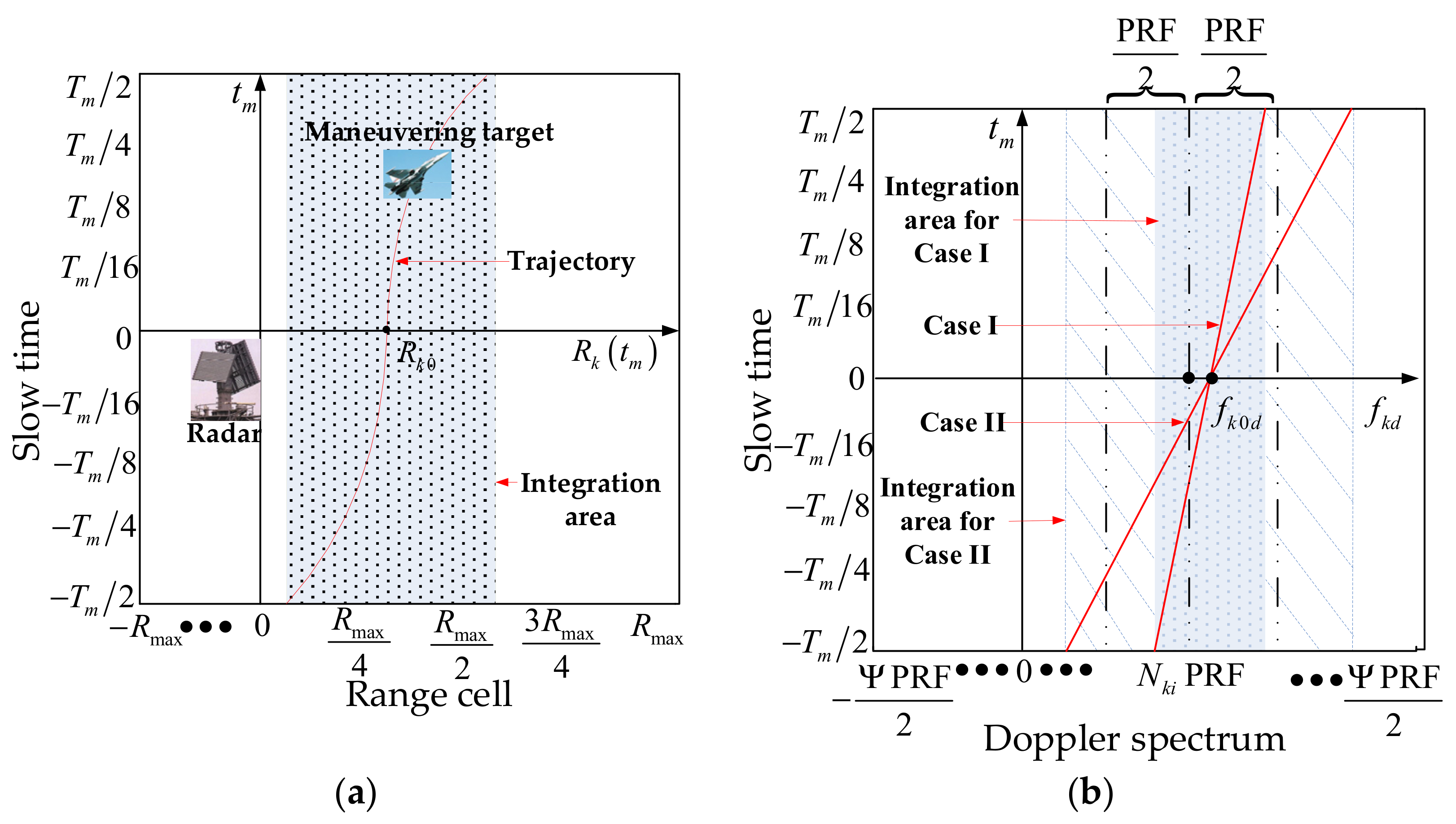
Suppose radar transmits the linear frequency modulated (LFM) signal waveform [36]

$$s_{trans}\left(\widehat{t}\right)=\mathrm{rect}\left(\frac{\widehat{t}}{T_p}\right)\exp \left[j2\pi \left(f_c\widehat{t}+\frac{1}{2}\gamma {\widehat{t}}^2\right)\right]$$

(1)

where $\mathrm{rect}\left(\frac{\widehat{t}}{T_p}\right)=\left\{\begin{array}{c}1,\left|\widehat{t}\right|\le T_p/2\\ 0,\left|\widehat{t}\right|>T_p/2\end{array}\right.$ is a rectangle window. $\widehat{t}$ is the fast time, i.e., the intra-pulse sampling time. $T_p$, $f_c$ and $\gamma$ denote the pulse duration, carrier frequency and frequency modulation rate, respectively.

The echo of K high-speed maneuvering targets after the down-conversion can be represented as

$$s_{recei}(\widehat{t},t_m)={\displaystyle \sum _{k=1}^K{A}_k\mathrm{rect}\left[\frac{\widehat{t}-{\tau }_{del,k}}{T_p}\right]}\exp \left\{j2\pi \left[-f_c{\tau }_{del,k}+\frac{1}{2}\gamma {\left(\widehat{t}-{\tau }_{del,k}\right)}^2\right]\right\}+n\left(\widehat{t},t_m\right)$$

(2)

where $t_m\in \left[-T_m/2,T_m/2\right]$ is the slow time, i.e., the inter-pulse sampling time. $T_m$ denotes the integration time. $A_k$ is the received signal voltage. ${\tau }_{del,k}=2R_k\left(t_m\right)/c$, $c$ is the speed of light, and $R_k\left(t_m\right)$ is the slant range between the kth target and radar at the instantaneous slow time $t_m$. $n\left(\widehat{t},t_m\right)$ denotes the additive stationary zero-mean complex white Gaussian noise of the power ${\sigma }_n^2$. According to the radar equation [17], we have the SNR for each target in Equation (2) as

$${\rho }_k=\frac{A_k^2}{{\sigma }_n^2}=\frac{P_t{G}^2{\lambda }^2\sigma }{{\left(4\pi \right)}^3{B}_c{T}_{e}BF{L}_s{R}_{k0}{}^4}$$

(3)

where $P_t$, $G$ and $\sigma$ are the radar transmission power, antenna gain and backscattering radar cross section, respectively. $\lambda =c/f_c$ denotes the wavelength. $B_c$, $T_e$, $F$, $L_s$ and $R_{k0}$ denote the Boltzmann constant, system Kelvin temperature, receiver noise figure, system loss and initial slant range, respectively.

Performing the range compression to Equation (2), we obtain the compressed signal in the fast time-slow time ($\widehat{t}$ ‑ $t_m$) domain as

$$s_{com}(\widehat{t},t_m)={\displaystyle \sum _{k=1}^K{A}_{k}B{T}_p}\mathrm{sinc}\left[B\left(\widehat{t}-{\tau }_{del,k}\right)\right]\exp \left(-j2\pi f_c{\tau }_{del,k}\right)+n_{com}\left(\widehat{t},t_m\right)$$

(4)

where $\mathrm{sinc}\left(x\right)=\sin \left(\pi x\right)/\left(\pi x\right)$. $n_{com}\left(\widehat{t},t_m\right)$ denotes the noise. After the range compression, the SNR for each target in Equation (4) is

$${\rho }_{rm,k}=B{T}_p\frac{A_k^2}{{\sigma }_n^2}=B{T}_p{\rho }_k$$

(5)

During the illumination time, the time-varying range $R_k\left(t_m\right)$ could be modeled as a multivariate function with $N+2$ unknown parameters $\left(R_{k0},v_{k0},a_{k1},\cdots ,a_{kN}\right)$ [17]. Since the illumination time is usually short, a second-order model is enough for realistic applications. However, we cannot deny that the higher the order is, the more accurate the time-varying range is.

$$R_k\left(t_m\right)=R_{k0}+v_{k0}{t}_m+\frac{a_{k1}}{2}{t}_m{}^2+\cdots +\frac{a_{kN}}{\left(N+1\right)!}{t}_m{}^{N+1}$$

(6)

where $v_{k0}$ denotes the radial velocity. $a_{k1},\cdots \mathrm{and} a_{kN}$ denote radial high-order motions.

Substituting Equation (6) into Equation (4) yields

$$\begin{array}{cc}\hfill s_{com}(\widehat{t},t_m)& ={\displaystyle \sum _{k=1}^K{A}_{k}B{T}_p}\hfill \\ & \times \mathrm{sinc}\left[B\left(\widehat{t}-\frac{2R_{k0}+2v_{k0}{t}_m+a_{k1}{t}_m{}^2+\cdots +\frac{2a_{kN}}{\left(N+1\right)!}{t}_m{}^{N+1}}{c}\right)\right]\hfill \\ & \times \exp \left(-j2\pi \frac{2R_{k0}+2v_{k0}{t}_m+a_{k1}{t}_m{}^2+\cdots +\frac{2a_{kN}}{\left(N+1\right)!}{t}_m{}^{N+1}}{\lambda }\right)\hfill \\ & +n_{com}\left(\widehat{t},t_m\right)\hfill \end{array}$$

(7)

The radar high-speed maneuvering target detection and localization model presented in Equation (7) is also widely used in SAR and ISAR imaging [38,39]. If the long-time coherent integration is perfectly carried out for $s_{com}(\widehat{t},t_m)$, the SNR for each target will be

$${\rho }_{cl,k}=B{T}_p{T}_m\mathrm{PRF}\frac{A_k^2}{{\sigma }_n^2}=B{T}_p{T}_m\mathrm{PRF}{\rho }_k$$

(8)

where $\mathrm{PRF}$ denotes the pulse repetition frequency.

Unfortunately, target motions induce the RCM and DFM, and the signal energy cannot be coherently integrated via performing the Fourier transform on $s_{com}(\widehat{t},t_m)$ along $t_m$. For the long-time coherent integration, many successful coherent methods have been proposed [16,17,18,19,20,21,22,23,24,25,26,27,28,29,30,31,32,33,34,35]. Referring to the published literature and conducting analyses of Equation (7), we summarize interference factors to realize the long-time integration and list them below for further research.

2.1. RCM and DFM

The target motions $\left(v_{k0},a_{k1},\cdots ,a_{kN}\right)$ influence the long-time coherent integration from two aspects, e.g., the envelop and Doppler spectrum. In Equation (7), the envelop offset is $v_{k0}{t}_m+a_{k1}{t}_m{}^2/2$ $+\cdots +\frac{2a_{kN}}{\left(N+1\right)!}{t}_m{}^{N+1}$. When the envelop offset exceeds the range resolution $c/2B$, the RCM happens [see Figure 1a]. The Doppler spread is $\left[2a_{k1}{t}_m+\cdots +\frac{2a_{kN}}{N!}{t}_m{}^N\right]/\lambda$ in Equation (7). When the Doppler spread exceeds the Doppler resolution $1/T_m$, the DFM happens (see Figure 1b). The RCM and DFM degrade the long-time coherent integration. In Figure 1a,b, $R_{\max }$ is the maximum value of $R_k\left(t_m\right)$, and $N_{ki}$ and $\mathrm{\Psi }$ correspond to the searching number and maximum searching range of the ambiguity integer, respectively.

2.2. Doppler Ambiguity Integer

The exponential term in Equation (7) can be rewritten as

$$\begin{array}{l}\exp \left(-j2\pi f_c\frac{2R_{k0}+2v_{k0}{t}_m+a_{k1}{t}_m{}^2+\cdots +\frac{2a_{kN}}{\left(N+1\right)!}{t}_m{}^{N+1}}{c}\right)\\ =\exp \left(-j4\pi \frac{f_c}{c}{R}_{k0}\right)\exp \left[-j2\pi \left(f_{k0}{t}_m+f_{k1}{t}_m{}^2+\cdots +f_{kN}{t}_m{}^{N+1}\right)\right]\end{array}$$

(9)

where $f_{k0}=2v_{k0}/\lambda$, $f_{k1}=a_{k1}/\lambda$, $f_{kN}=2a_{kN}/\left[\left(N+1\right)!\lambda \right]$.

If the velocity is ambiguous (this easily happens under the high speed, large carrier frequency or low PRF) [37], the instantaneous Doppler of the kth target should be represented as

$$f_{kd}=\frac{d\left(f_{k0}{t}_m+f_{k1}{t}_m{}^2+\cdots +f_{kN}{t}_m{}^{N+1}\right)}{d{t}_m}=f_{k0d}+2f_{k1}{t}_m+\cdots +\left(N+1\right)f_{kN}{t}_m{}^N+N_{k0d}\mathrm{PRF}$$

(10)

where $f_{k0d}$ and $N_{k0d}$ denote the ambiguous Doppler and ambiguity integer, respectively. Equation (10) indicates that, if the velocity is ambiguous, there will be an ambiguity integer. According to [36,37], the Doppler ambiguity integer makes the long-time coherent integration complicated, such as the BSSL (see Figure 1c) and the following two problems. It is worthwhile noting the BSSL appears mainly because the RCM compensation and the coherent integration along the slow time correspond to two different velocity resolutions. This will be theoretically interpreted in Section 3.

2.3. Doppler Spectrum Coupling and Half-Blind-Velocity Effect

The item $2f_{k1}{t}_m+\cdots +\left(N+1\right)f_{kN}{t}_m{}^N$ couples with $f_{k0d}$ in Equation (10), which categories the Doppler spectrum into two cases [see Figure 1b], Case I: $f_{k0d}+2f_{k1}{t}_m+\cdots +$ $\left(N+1\right)f_{kN}{t}_m{}^N$ is entirely in a PRF band, and Case II: $f_{k0d}+2f_{k1}{t}_m+\cdots +\left(N+1\right)f_{kN}{t}_m{}^N$ spans more than one PRF band. Case II, i.e., Doppler spectrum coupling, may disable KT-based methods [24,25,26].

The equation $f_{k0}=f_{k0d}+N_{k0d}\mathrm{PRF}$ is based on the assumption that the bandwidth has no influence on the wavelength. However, a high bandwidth may influence the wavelength and $f_{k0}$ may span several PRF bands when $f_{k0d}$ is close to $\mathrm{PRF}/2$. We call this effect as the half-blind-velocity effect [26].

Under the Doppler spectrum coupling and the half-blind-velocity effect, the ambiguity integer is not constant anymore. However, KT-based methods are based on the assumption that the ambiguity integer is constant. Therefore, under this condition, the ergodic searching of the ambiguity integer cannot compensate the linear RCM clearly after the KT-based methods.

3. PU Mode and PS Mode

In this section, we deduce closed analytical formulae of two typical detection and localization methods, i.e., the MLE method and KTD method, for a better understanding of the PU mode and PS mode. With closed analytical formulae, several doubts in radar high-speed maneuvering target detection and localization will be interpreted.

3.1. PU Mode

The signal expression of $s_{com}(\widehat{t},t_m)$ in the range frequency-slow time domain can be written as

$$\begin{array}{cc}\hfill S_c\left(f,t_m\right)& ={\displaystyle \sum _{k=1}^K{A}_k\mathrm{rect}\left[\frac{f}{\gamma T_p}\right]}\exp \left(-j2\pi \frac{f+f_c}{c}{f}_{k0}\lambda t_m\right)\hfill \\ & \times \exp \left[-j4\pi \frac{f+f_c}{c}\left(R_{k0}+\frac{a_{k1}}{2}{t}_m{}^2+\cdots +\frac{a_{kN}}{\left(N+1\right)!}{t}_m{}^{N+1}\right)\right]\hfill \\ & +n_c\left(f,t_m\right)\hfill \end{array}$$

(11)

where $f$ denotes the range frequency. $n_c\left(f,t_m\right)$ denotes the noise in the range frequency-slow time domain.

It is easily seen from Equation (11) that the linear RCM compensation and inter-pulse energy integration can be done via the ergodic searching of the unknown $f_{k0}$. This is the basic principle of the PU mode. Referring to the literature [5,6] and [16,17,18,19], we present the general form of the PU mode as

$$P\mathrm{U}\left({\widehat{f}}_0,〈\cdots 〉\right)=O{P}_2\left\{O{P}_1\left[S_c\left(f,t_m\right)\right]\exp \left[j2\pi \frac{\left(f+f_c\right)}{c}{\widehat{f}}_0\lambda t_m\right]\right\}$$

(12)

where ${\widehat{f}}_0$ denotes the searching variable of $f_{k0}$.$〈\cdots 〉$ denotes other searching variables. $O{P}_1\left[•\right]$ and $O{P}_2\left[•\right]$ denote two operations, such as the dechirp, integration, and so on [5,6].

For a better understanding of the PU mode and its general form, we consider a typical method of the PU mode, i.e., MLE method. It can be presented as

$$\begin{array}{l}\mathrm{MLE}\left({\widehat{f}}_0,{\widehat{R}}_0,{\widehat{a}}_1,\cdots ,{\widehat{a}}_N\right)=\underset{¯}{\underset{¯}{{\displaystyle \underset{t_m}{\int }{\displaystyle \underset{f}{\int }}}}}{S}_c\left(f,t_m\right)\underset{¯}{\exp \left[j2\pi \frac{\left(f+f_c\right)}{c}\right.}\\ \underset{¯}{\left.\times \left(2{\widehat{R}}_0+{\widehat{a}}_1{t}_m{}^2+\cdots +\frac{2{\widehat{a}}_N}{\left(N+1\right)!}{t}_m{}^{N+1}\right)\right]}\exp \left[j2\pi \frac{\left(f+f_c\right)}{c}{\widehat{f}}_0\lambda t_m\right]\underset{¯}{\underset{¯}{dfd{t}_m}}\end{array}$$

(13)

where ${\widehat{R}}_0,{\widehat{a}}_1,\cdots ,\mathrm{and}{\widehat{a}}_N$ denote searching variables of $R_{k0},a_{k1},\cdots , \mathrm{and} a_{kN}$, respectively. The target is non-cooperative and we do not have its motion parameters. Therefore, in realistic applications, we set the searching range and interval for ${\widehat{R}}_0,{\widehat{a}}_1,\cdots , \mathrm{and} {\widehat{a}}_N$ to match $R_{k0},a_{k1},\cdots , \mathrm{and} a_{kN}$. For the detailed implementation, we can refer to Section 4.2. In the MLE method, the dechirp operation marked with the single underline corresponds to $O{P}_1\left[•\right]$ and the integration marked with double underline corresponds to $O{P}_2\left[•\right]$.

Substituting $S_c\left(f,t_m\right)$ into Equation (13), we obtain the closed analytical formula of the MLE method as

$$\begin{array}{l}\mathrm{MLE}\left({\widehat{f}}_0,{\widehat{R}}_0,{\widehat{a}}_1,\cdots ,{\widehat{a}}_N\right)={\displaystyle \sum _{k=1}^K{A}_{k}B{T}_p{T}_m\mathrm{PRF}}\\ \times \mathrm{sinc}\left[\frac{2B}{c}\left({\widehat{R}}_0-R_{k0}\right)\right]\mathrm{sinc}\left[\frac{T_m^2{f}_c}{4c}\left({\widehat{a}}_1-a_{k1}\right)\right]\\ \times \cdots \mathrm{sinc}\left[\frac{T_m^2{f}_c}{2^N\left(N+1\right)!c}\left({\widehat{a}}_N-a_{kN}\right)\right]\\ \underleftrightarrow{\underleftrightarrow{\times \mathrm{sinc}\left[\frac{2B{T}_m}{3c}\frac{\lambda }{2}\left({\widehat{f}}_0-f_{k0}\right)\right]\mathrm{sinc}\left\{T_m\left\{\mathrm{mod}\left[\left({\widehat{f}}_0-f_{k0}\right)/\mathrm{PRF}\right]\right\}\right\}}}\\ +n_M\left({\widehat{f}}_0,{\widehat{R}}_0,{\widehat{a}}_1,\cdots ,{\widehat{a}}_N\right)\end{array}$$

(14)

where $\mathrm{mod}\left[\left({\widehat{f}}_0-f_{k0}\right)/\mathrm{PRF}\right]$ returns the remainder after division of $\left({\widehat{f}}_0-f_{k0}\right)$ by $\mathrm{PRF}$.$n_M\left({\widehat{f}}_0,{\widehat{R}}_0,{\widehat{a}}_1,\cdots ,{\widehat{a}}_N\right)$ denotes the noise. Note that the second, third, and fifth sinc functions are only approximate expressions.

The signal energy is coherently integrated at $\left(f_{k0},R_{k0},a_{k1},\cdots ,a_{kN}\right)$ after the MLE method. Note that ${\widehat{f}}_0$ appears in two sinc functions marked in Equation (14). The resolution of ${\widehat{f}}_0$ is $3f_c/\left(B{T}_m\right)$ in the first sinc function, while it is $1/T_m$ in the second sinc function. Since $f_c$ is larger than $B$, $3f_c/\left(B{T}_m\right)$ is larger than $1/T_m$. Therefore, along ${\widehat{f}}_0$, the first sinc function determines the outside contour and the second sinc function samples this outside contour with the interval $\mathrm{PRF}$, i.e., $1/T_m$. Here, we use a numerical example to illustrate the ${\widehat{f}}_0$ dimension of Equation (14).

Example 1:

The radar parameters are set as$f_c=4\mathrm{GHz}$,$\mathrm{PRF}=200\mathrm{Hz}$and$B=15\mathrm{MHz}$. The number of integrated pulses is 200.$v_{k0}=39m/s$($f_{k0}=2v_{k0}/\lambda =1040\mathrm{Hz}$). In Figure 2, the top left figure illustrates the first sinc function marked in Equation (14), the top right figure illustrates the second sinc function marked in Equation (14), and the bottom figure illustrates the energy distribution along${\widehat{f}}_0$.

In the bottom figure of Figure 2, besides the peak at ${\widehat{f}}_0=1040\mathrm{Hz}$, many high sidelobes appear and are right located around ambiguity integer times. They are known as BSSLs which are samples of the first sinc function via the second sinc function marked in Equation (14). Obviously, BSSLs may influence the target detection and localization when we use the constant false alarm rate (CFAR) technique. As we know, the peak-to-first sidelobe ratio along the range dimension is about 13 dB and the influence of the sidelobe can be ignored. Therefore, we refer to this phenomenon and set radar parameters to let the ratio between the peak and BSSLs higher than 13 dB. The width of a sinc function at −13 dB is about twice the resolution. In addition, the interval between two adjacent samples of the first sinc function is $\mathrm{PRF}$. Therefore, if the following Equation (15) holds, the influence of BSSLs may be ignored via a CFAR method.

$$\mathrm{PRF}\ge \frac{3f_c}{B{T}_m}\iff M\ge \frac{3f_c}{B}$$

(15)

where $T_m=M/\mathrm{PRF}$ and $M$ denotes the number of the integrated pulses. Equation (15) indicates that we may eliminate the influence of BSSLs via adjusting $M$, $f_c$ and $B$.

Remark 1:

The reference [37] also analyze BSSLs and two approaches, i.e., system parameter design and weighting function, are proposed for the BSSLs suppression. Our work can be seen as an extension of [37]. Compared to its work, our work is characterized by (1) the clearer interpretation of the BSSLs, i.e., the searching variable${\widehat{f}}_0$has two different resolutions; and (2) the explicit system parameter design, i.e., the Equation (15).

Above is the analysis of the PU mode via the MLE method. The problem of BSSLs is clearly interpreted and an explicit system parameter design is presented also. In the following subsection, we will analyze the PS mode via the KTD method.

3.2. PS Mode

The first exponential term of Equation (11) can be divided into two exponential terms, one corresponds to the linear RCM and the other corresponds to the inter-pulse energy integration. Basing on this characteristic, we rewrite $S_c\left(f,t_m\right)$ as

$$\begin{array}{l}{S}_c\left(f,t_m\right)={\displaystyle \sum _{k=1}^K{A}_k\mathrm{rect}\left[\frac{f}{\gamma T_p}\right]}\exp \left(-j4\pi \frac{f}{c}{v}_{k0}{t}_m\right)\exp \left(-j2\pi f_{k0d}{t}_m\right)\\ \times \exp \left[-j4\pi \frac{f+f_c}{c}\left(R_{k0}+\frac{a_{k1}}{2}{t}_m{}^2+\cdots +\frac{a_{kN}}{\left(N+1\right)!}{t}_m{}^{N+1}\right)\right]+n_c\left(f,t_m\right)\end{array}$$

(16)

where $\exp \left(j2\pi N_{k0d}\mathrm{PRF}{t}_m\right)=1$ is ignored.

In Equation (16), the first exponential term corresponds to the linear RCM and the second exponential term corresponds to the inter-pulse energy integration. Therefore, we can use two different physical variables to separately perform the linear RCM compensation and inter-pulse energy integration. This is the basic principle of the PS mode. Referring to the literature [24,25,26] and [29,30,31,32,33,34,35], we present the general form of the PS mode as

$$\mathrm{PS}\left({\widehat{f}}_{0d},\widehat{𝓁},〈\cdots 〉\right)=O{P}_4\left\{O{P}_3\left[S_c\left(f,t_m\right)\right]\exp \left(j2\pi \frac{f}{c}\widehat{𝓁}{t}_m\right)\exp \left(j2\pi {\widehat{f}}_{0d}{t}_m\right)\right\}$$

(17)

where ${\widehat{f}}_{0d}$ denotes the searching variable of $f_{k0d}$. $\widehat{𝓁}$ denotes the searching variable for the linear RCM compensation. $O{P}_3\left[•\right]$ and $O{P}_4\left[•\right]$ denote two operations, such as the dechirp, autocorrelation, integration, and so on [24,25,26,29,30,31,32,33,34,35]. Note that $\widehat{𝓁}$ is only a symbol and the actual searching variable depends on the specific method. For example, for KT-based methods [24,25,26], $\widehat{𝓁}=\lambda {\widehat{N}}_{0d}\mathrm{PRF}$ and the actual searching variable is ${\widehat{N}}_{0d}$ (i.e., the searching variable of $N_{k0d}$, ${\widehat{N}}_{0d}=-\left[N_{{\widehat{N}}_{0d}}/2\right],-\left[N_{{\widehat{N}}_{0d}}/2\right]+1,\dots ,\left[\left(N_{{\widehat{N}}_{0d}}-1\right)/2\right]$, $N_{{\widehat{N}}_{0d}}$ denote searching times for the unknown parameters $N_{k0d}$), while for the scaled inverse Fourier transform-based method [34,35], $\widehat{𝓁}=2{\widehat{v}}_0$ and the actual searching variable is ${\widehat{v}}_0$ (i.e., the searching variable of $v_{k0}$).

For a better understanding of the PS mode and its general form, we consider a typical method of the PU mode, i.e., the KTD method. It can be presented as

$$\begin{array}{l}KTD\left({\widehat{f}}_{0d},{\widehat{N}}_{0d},{\widehat{R}}_0,{\widehat{a}}_1,\cdots ,{\widehat{a}}_N\right)=\underset{=}{{{\displaystyle \int }}_{{\tau }_m}{{\displaystyle \int }}_f}\left[\underset{¯}{{{\displaystyle \int }}_{{\widehat{f}}_{0d}}{{\displaystyle \int }}_{t_m}{S}_c\left(f,t_m\right)}\right.\\ \hspace{1em}\hspace{1em}\hspace{1em}\hspace{1em}\underset{¯}{\left.\times \exp \left(j2\pi {\widehat{f}}_{0d}\frac{f+f_c}{f_c}{t}_m\right)\exp \left(j2\pi {\widehat{f}}_{0d}{\tau }_m\right)\right]d{t}_{m}d{\widehat{f}}_{0d}}\\ \hspace{1em}\hspace{1em}\hspace{1em}\hspace{1em}\underset{=}{\times \exp \left\{j2\pi \frac{\left(f+f_c\right)}{c}\left[2{\widehat{R}}_0+{\widehat{a}}_1{\left(\frac{f_c}{f+f_c}{\tau }_m\right)}^2\right.\right.}\\ \hspace{1em}\hspace{1em}\hspace{1em}\hspace{1em}\underset{=}{\left.\left.+\cdots +\frac{2{\widehat{a}}_N}{\left(N+1\right)!}{\left(\frac{f_c}{f+f_c}{\tau }_m\right)}^{N+1}\right]\right\}}\\ \hspace{1em}\hspace{1em}\hspace{1em}\hspace{1em}\times \exp \left(j2\pi \frac{f}{c}\lambda {\widehat{N}}_{0d}PRF{\tau }_m\right)\exp \left(j2\pi {\widehat{f}}_{0d}{\tau }_m\right)\underset{=}{dfd{\tau }_m}\end{array}$$

(18)

where ${\tau }_m$ denotes a scaled variable corresponding to $t_m$. In the KTD method, the KT operation marked with the single underline corresponds to $O{P}_3\left[•\right]$, and the dechirp operation and integration marked with double underline correspond to $O{P}_4\left[•\right]$.

We substitute $S_c\left(f,t_m\right)$ into Equation (18) and obtain the closed analytical formula of the KTD method as

$$\begin{array}{l}\mathrm{KT}\mathrm{D}\left({\widehat{f}}_{0d},{\widehat{N}}_{0d},{\widehat{R}}_0,{\widehat{a}}_1,\cdots ,{\widehat{a}}_N\right)\approx {\displaystyle \sum _{k=1}^K{A}_{k}B{T}_p{T}_m}\mathrm{PRF}\\ \hspace{1em}\hspace{1em}\hspace{1em}\hspace{1em}\times \mathrm{sinc}\left[\frac{2B}{c}\left({\widehat{R}}_0-R_{k0}\right)\right]\mathrm{sinc}\left[\frac{T_m^2{f}_c}{4c}\left({\widehat{a}}_1-a_{k1}\right)\right]\\ \hspace{1em}\hspace{1em}\hspace{1em}\hspace{1em}\times \cdots \mathrm{sinc}\left[\frac{T_m^2{f}_c}{2^N\left(N+1\right)!c}\left({\widehat{a}}_N-a_{kN}\right)\right]\\ \underleftrightarrow{\underleftrightarrow{\times \mathrm{sinc}\left[\frac{2B{T}_m}{3c}\frac{\lambda \mathrm{PRF}}{2}\left({\widehat{N}}_{0d}-N_{k0d}\right)\right]\mathrm{sinc}\left[T_m\left({\widehat{f}}_{0d}-f_{k0d}\right)\right]}}\\ \hspace{1em}\hspace{1em}\hspace{1em}\hspace{1em}+n_K\left({\widehat{f}}_{0d},{\widehat{N}}_{0d},{\widehat{R}}_0,{\widehat{a}}_1,\cdots ,{\widehat{a}}_N\right)\end{array}$$

(19)

where $n_K\left({\widehat{f}}_{0d},{\widehat{N}}_{0d},{\widehat{R}}_0,{\widehat{a}}_1,\cdots ,{\widehat{a}}_N\right)$ denotes the noise. Note that the second, third, and fourth sinc functions are only approximate expressions.

The signal energy after the KTD method is coherently integrated at $\left(N_{k0d},f_{k0d},R_{k0},a_{k1},\cdots ,a_{kN}\right)$. Two parameter dimensions, i.e., ${\widehat{N}}_{0d}$ and ${\widehat{f}}_{0d}$, appear in the KTD method instead of one parameter dimension, i.e., ${\widehat{f}}_0$, in the MLE method. Comparing Equation (19) with Equation (14), we find that the signal energy distribution along ${\widehat{N}}_{0d}$ can be seen as extractions of the ${\widehat{f}}_0$ dimension at ambiguity integers and the signal energy distribution along ${\widehat{f}}_{0d}$ can be seen as extractions of the ${\widehat{f}}_0$ dimension in $\left[-\mathrm{PRF}/2,\mathrm{PRF}/2\right)$. Here, we use a numerical example to illustrate ${\widehat{N}}_{0d}$ and ${\widehat{f}}_{0d}$ dimensions of Equation (19).

Example 2:

The radar and motion parameters are set as those of Example 1. The number of integrated pulses is also 200. In Figure 3, the top left figure shows the signal energy distribution along${\widehat{N}}_{0d}$, the top right figure shows the signal energy distribution along${\widehat{f}}_{0d}$, and the bottom figure illustrates the signal energy distribution in the${\widehat{N}}_{0d}-{\widehat{f}}_{0d}$domain.

Extractions of the ${\widehat{f}}_0$ dimension at ambiguity integers are also plotted with the red line in the top left figure of Figure 3. As analyzed above, the signal energy distribution along ${\widehat{N}}_{0d}$ can be seen as extractions of the ${\widehat{f}}_0$ dimension at ambiguity integers. Based on Equations (14) and (19), and related analyses and results shown in Figure 2 and Figure 3, it is not difficult to find that the KTD method and the MLE method have the same energy integration, while the searching range of ${\widehat{f}}_{0d}$ is fixed into $\left[-\mathrm{PRF}/2,\mathrm{PRF}/2\right)$ and the searching procedure for $f_{k0d}$ can be speed up via the fast Fourier transform (FFT) [24,25,26,29,30,31,32,33,34,35]. That is, these two methods have the same energy integration, while the KTD method is more computationally efficient than the MLE method.

Remark 2:

Several published studies claim that their KT-based methods can eliminate BSSLs. Based on analyses above, we know that, in KT-based methods, the BSSLs disappear along the ambiguous Doppler${\widehat{f}}_{0d}$dimension, while they still exist along the ambiguity integer${\widehat{N}}_{0d}$dimension.

Remark 3:

Note that we use$“\approx ”$instead of$“=”$in Equation (19). This is because Equation (19) is conditional, i.e., the Doppler spectrum coupling and half-blind-velocity effect do not happen. If these two problems happen, the signal energy after the KTD method may spread. In Section 5, we will use numerical simulations to demonstrate drawbacks of the KTD method.

Above is the analysis of the PU mode and PS mode with two typical methods, i.e., the MLE method and the KTD method. Compared to the PU mode, the PS mode is more computationally efficient. However, its representative method, i.e., the KTD method, may encounter anti-noise performance loss when the Doppler spectrum coupling and half-blind-velocity effect happen. In the following, we continue the research of the PS mode and propose a novel long-time coherent integration method, i.e., GDKT, which is statistically optimal and computationally efficient.

4. GDKT and Implementation

In this section, the GDKT belonging to the PS mode is proposed for radar high-speed maneuvering target detection and localization. A fast implementation method is also presented for the GDKT.

4.1. GDKT

The KT-based methods are based on the assumption that the ambiguity integer is constant. However, due to the Doppler spectrum coupling and half-blind-velocity effect, the ambiguity integer may not be constant and the ergodic searching of the unknown ambiguity integer cannot compensate for the linear RCM clearly [24,25,26,27]. Without doubt, if the influence of the Doppler spectrum coupling and half-blind-velocity effect can be eliminated before the KT, the proposed KT-based method will be statistically optimal and computationally efficient. Under such a guideline, we propose a novel coherent method, known as the GDKT.

$$\begin{array}{l}\mathrm{GD}\mathrm{KT}\left({\widehat{f}}_{0d},{\widehat{v}}_0,{\widehat{R}}_0,{\widehat{a}}_1,\cdots ,{\widehat{a}}_N\right)=\underset{¯}{\underset{¯}{{\displaystyle \underset{f}{\int }{\displaystyle \underset{t_m}{\int }}}}}{S}_c\left(f,t_m\right)\\ \hspace{1em}\hspace{1em}\hspace{1em}\hspace{1em}\underset{¯}{\left.\times \exp \left[j2\pi \frac{\left(f+f_c\right)}{c}\right.\left(2{\widehat{R}}_0+{\widehat{a}}_1{t}_m{}^2+\cdots +\frac{2{\widehat{a}}_N}{\left(N+1\right)!}{t}_m{}^{N+1}\right)\right]}\\ \hspace{1em}\hspace{1em}\hspace{1em}\hspace{1em}\underset{¯}{\times \exp \left(j2\pi \frac{f}{c}\lambda {\widehat{N}}_{0d}\mathrm{PRF}{t}_m\right)}\exp \left(j2\pi {\widehat{f}}_{0d}\frac{f+f_c}{f_c}{t}_m\right)\underset{=}{d{t}_{m}df}\end{array}$$

(20)

In the GDKT, the dechirp operation marked with single underline corresponds to $O{P}_3\left[•\right]$ and the integration marked with double underline corresponds to $O{P}_4\left[•\right]$. Note that the first exponential term used in the dechirp operation can eliminate the influence of the Doppler spectrum coupling and the second exponential term used in the dechirp operation can eliminate the influence of half-blind-velocity effect.

We substitute $S_c\left(f,t_m\right)$ into Equation (20) and obtain the closed analytical formula of the GDKT as

$$\begin{array}{l}\mathrm{GD}\mathrm{KT}\left({\widehat{f}}_{0d},{\widehat{N}}_{0d},{\widehat{R}}_0,{\widehat{a}}_1,\cdots ,{\widehat{a}}_N\right)={\displaystyle \sum _{k=1}^K{A}_{k}B{T}_p{T}_m}\mathrm{PRF}\\ \hspace{1em}\hspace{1em}\hspace{1em}\hspace{1em}\times \mathrm{sinc}\left[\frac{2B}{c}\left({\widehat{R}}_0-R_{k0}\right)\right]\mathrm{sinc}\left[\frac{T_m^2{f}_c}{4c}\left({\widehat{a}}_1-a_{k1}\right)\right]\\ \hspace{1em}\hspace{1em}\hspace{1em}\hspace{1em}\times \cdots \mathrm{sinc}\left[\frac{T_m^2{f}_c}{2^N\left(N+1\right)!c}\left({\widehat{a}}_N-a_{kN}\right)\right]\\ \underleftrightarrow{\underleftrightarrow{\times \mathrm{sinc}\left[\frac{2B{T}_m}{3c}\frac{\lambda \mathrm{PRF}}{2}\left({\widehat{N}}_{0d}-N_{k0d}\right)\right]\mathrm{sinc}\left[T_m\left({\widehat{f}}_{0d}-f_{k0d}\right)\right]}}\\ \hspace{1em}\hspace{1em}\hspace{1em}\hspace{1em}+n_G\left({\widehat{f}}_{0d},{\widehat{N}}_{0d},{\widehat{R}}_0,{\widehat{a}}_1,\cdots ,{\widehat{a}}_N\right)\end{array}$$

(21)

where $n_G\left({\widehat{f}}_{0d},{\widehat{N}}_{0d},{\widehat{R}}_0,{\widehat{a}}_1,\cdots ,{\widehat{a}}_N\right)$ denotes the noise. Note that the second, third, and fourth sinc functions are only approximate expressions.

The closed analytical formula of the GDKT method is the same as that of the KTD method, except $“=”$. The signal energy after the GDKT is coherently integrated at $\left(N_{k0d},f_{k0d},R_{k0},a_{k1},\cdots ,a_{kN}\right)$. Compared to the KTD method, the GDKT is statistically optimal. Since example 2 does not take the influence of the Doppler spectrum coupling and half-blind-velocity effect into consideration, results shown in Figure 3 can also illustrate ${\widehat{v}}_0$ and ${\widehat{N}}_{0d}$ dimensions of Equation (21).

Now, the CFAR technique can be used to do the target detection and localization. Compare $\mathrm{GD}\mathrm{KT}\left({\widehat{f}}_{0d},{\widehat{N}}_{0d},{\widehat{R}}_0,{\widehat{a}}_1,\cdots ,{\widehat{a}}_N\right)$ with the threshold value $\eta$ (can be easily calculated with the false alarm rate and noise power of reference cells). For more details of the CFAR, the readers can refer to [2,3,4].

$$\left|\mathrm{GD}\mathrm{KT}\left({\widehat{f}}_{0d},{\widehat{N}}_{0d},{\widehat{R}}_0,{\widehat{a}}_1,\cdots ,{\widehat{a}}_N\right)\right|\underset{H_0}{\overset{H_1}{\gtrless }}\eta$$

(22)

If $\left|\mathrm{GD}\mathrm{KT}\left({\widehat{f}}_{0d},{\widehat{N}}_{0d},{\widehat{R}}_0,{\widehat{a}}_1,\cdots ,{\widehat{a}}_N\right)\right|$ is larger than $\eta$, there will be a target. Meanwhile, all the motion and localization parameters can be directly estimated. On the contrary, if $\left|\mathrm{GD}\mathrm{KT}\left({\widehat{f}}_{0d},{\widehat{N}}_{0d},{\widehat{R}}_0,{\widehat{a}}_1,\cdots ,{\widehat{a}}_N\right)\right|$ is smaller than $\eta$, there will be no target. Note that the BSSLs do exist in the GDKT and may influence the CFAR. In this paper, we base on the deduced Equation (15) and propose to eliminate the influence of the BSSLs by extending the integration time $T_m$.

Compared to the MLE method and the KTD method, the GDKT has two main superiorities, including

• The GDKT uses ${\widehat{v}}_0$ and ${\widehat{f}}_{0d}$ to separately process the linear RCM and inter-pulse energy integration. Similar to the KTD method, the GDKT is more computationally efficient than the MLE method;
• In the GDKT, the KT is employed after eliminating the influence of the Doppler spectrum coupling and half-blind-velocity effect. Therefore, same as the MLE method, the GDKT is statistically optimal.

Above is the proposed GDKT for radar high-speed maneuvering target detection and localization. In the following subsection, we will present an implementation method for the GDKT.

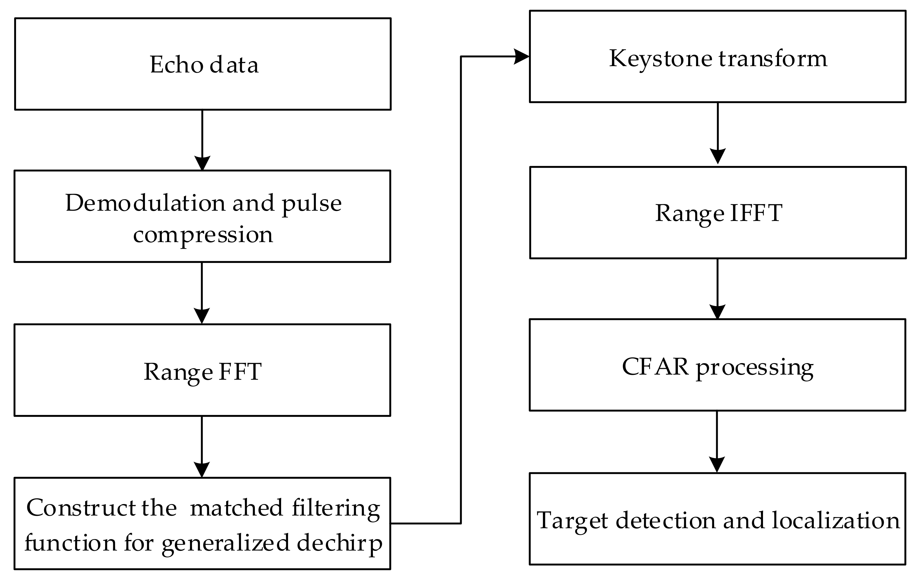
4.2. Implementation of the GDKT

The key steps of the GDKT are the dechirp and KT operations. In this subsection, we present an implementation method for the GDKT. Based on the sampling scheme of Claasen and Mecklenbrauker [38], the discrete form of can be expressed as

$$\begin{array}{cc}\hfill S_c\left(n_f,n_{t_m}\right)& ={\displaystyle \sum _{k=1}^K{B}_k\mathrm{rect}\left[\frac{n_f{\Delta }_f}{\gamma T_p}\right]}\exp \left(-j2\pi f_{k0d}{n}_{t_m}{\Delta }_{t_m}\right)\hfill \\ & \times \exp \left(-j4\pi \frac{n_f{\Delta }_f}{c}{R}_{k0}\right)\exp \left(-j4\pi \frac{n_f{\Delta }_f}{c}{v}_{k0}{n}_{t_m}{\Delta }_{t_m}\right)\hfill \\ & \times \exp \left\{-j4\pi \frac{n_f{\Delta }_f+f_c}{c}\left[\frac{a_{k1}}{2}{\left(n_{t_m}{\Delta }_{t_m}\right)}^2+\cdots +\frac{a_{kN}}{\left(N+1\right)!}{\left(n_{t_m}{\Delta }_{t_m}\right)}^{N+1}\right]\right\}\hfill \\ & +n_c\left(n_f,n_{t_m}\right)\hfill \end{array}$$

(23)

where $B_k=A_k\exp \left(-j4\pi R_{k0}{f}_c/c\right)$.${\Delta }_f$ and ${\Delta }_{t_m}$ denote sampling intervals of $f$ and $t_m$, respectively. $n_f=-\left[N_f/2\right],-\left[N_f/2\right]+1,\cdots ,\left[\left(N_f-1\right)/2\right]$. $N_f$ denotes the number of samplings of $f$. $n_{t_m}=-\left[M/2\right],-\left[M/2\right]+1,\cdots ,\left[\left(M-1\right)/2\right]$.

Step 1:

Construct the$N+3$-dimension matched filtering function.

$$\begin{array}{l}{G}_1\left(n_f,n_{t_m},{\widehat{N}}_{0d},n_{{\widehat{a}}_1},\cdots ,n_{{\widehat{a}}_N}\right)=\exp \left(j2\pi \frac{n_f{\Delta }_f}{c}\lambda {\widehat{N}}_{0d}\mathrm{PRF}{n}_{t_m}{\Delta }_{t_m}\right)\\ \times \exp \left\{j4\pi \frac{n_f{\Delta }_f+f_c}{c}\left[\frac{n_{{\widehat{a}}_1}{\Delta }_{{\widehat{a}}_1}}{2}{\left(n_{t_m}{\Delta }_{t_m}\right)}^2+\cdots +\frac{n_{{\widehat{a}}_N}{\Delta }_{{\widehat{a}}_N}}{\left(N+1\right)!}{\left(n_{t_m}{\Delta }_{t_m}\right)}^{N+1}\right]\right\}\end{array}$$

(24)

where ${\Delta }_{{\widehat{a}}_1}$ and ${\Delta }_{{\widehat{a}}_N}$ denote searching intervals for unknown parameters $a_{k1}$ and $a_{kN}$, respectively. We can refer to the parameter resolution to determine corresponding searching interval. $n_{{\widehat{a}}_1}=-\left[N_{{\widehat{a}}_1}/2\right],-\left[N_{{\widehat{a}}_1}/2\right]+1,\cdots ,\left[\left(N_{{\widehat{a}}_1}-1\right)/2\right]$. $n_{{\widehat{a}}_N}=-\left[N_{{\widehat{a}}_N}/2\right],-\left[N_{{\widehat{a}}_N}/2\right]+1,$ ⋯, $\left[\left(N_{{\widehat{a}}_N}-1\right)/2\right]$. $N_{{\widehat{a}}_1}$ and $N_{{\widehat{a}}_N}$ denote searching times for unknown parameters $a_{k1}$ and $a_{kN}$, respectively.

Step 2:

Multiply$G_1\left(n_f,n_{t_m},{\widehat{N}}_{0d},n_{{\widehat{a}}_1},\cdots ,n_{{\widehat{a}}_N}\right)$with$S_c\left(n_f,n_{t_m}\right)$.

$$S_{c1}\left(n_f,n_{t_m},{\widehat{N}}_{0d},n_{{\widehat{a}}_1},\cdots ,n_{{\widehat{a}}_N}\right)=S_c\left(n_f,n_{t_m}\right)G_1\left(n_f,n_{t_m},{\widehat{N}}_{0d},n_{{\widehat{a}}_1},\cdots ,n_{{\widehat{a}}_N}\right)$$

(25)

Step 3:

Apply the KT to$S_{c1}\left(n_f,n_{t_m},{\widehat{N}}_{0d},n_{{\widehat{a}}_1},\cdots ,n_{{\widehat{a}}_N}\right)$.

$$S_{c2}\left(n_f,n_{f_{t_m}},{\widehat{N}}_{0d},n_{{\widehat{a}}_1},\cdots ,n_{{\widehat{a}}_N}\right)={\displaystyle \sum _{n_{t_m}}{S}_{c1}\left(n_f,n_{t_m},{\widehat{N}}_{0d},n_{{\widehat{a}}_1},\cdots ,n_{{\widehat{a}}_N}\right)}\times \exp \left(j2\pi \frac{n_{f_{t_m}}}{M}\frac{n_f{\Delta }_f+f_c}{f_c}{n}_{t_m}\right)$$

(26)

where $n_{f_{t_m}}$ denotes samplings of $f_{t_m}$. $f_{t_m}$ is the frequency domain with respect to $t_m$. Note that the KT can be speeded up via the FFT-based chirp-z transform [20,21,22,23,24,25].

Step 4:

Perform the inverse FFT (IFFT) with respect to$n_f$.

$$\mathrm{GDKT}\left(n_{\widehat{t}},n_{f_{t_m}},{\widehat{N}}_{0d},n_{{\widehat{a}}_1},\cdots ,n_{{\widehat{a}}_N}\right)={\mathrm{IFFT}}_{n_f}\left[S_{c2}\left(n_f,n_{f_{t_m}},{\widehat{N}}_{0d},n_{{\widehat{a}}_1},\cdots ,n_{{\widehat{a}}_N}\right)\right]$$

(27)

where $n_{\widehat{t}}$ denotes samplings of the fast time $\widehat{t}$. $\mathrm{IFFT}\left[·\right]$ denotes the IFFT operation.

Step 5:

Compare$\mathrm{GDKT}\left(n_{\widehat{t}},n_{f_{t_m}},{\widehat{N}}_{0d},n_{{\widehat{a}}_1},\cdots ,n_{{\widehat{a}}_N}\right)$with the threshold value$\eta$determined by the CFAR to complete the target detection and localization.

$$\left|\mathrm{GDKT}\left(n_{\widehat{t}},n_{f_{t_m}},{\widehat{N}}_{0d},n_{{\widehat{a}}_1},\cdots ,n_{{\widehat{a}}_N}\right)\right|\underset{H_0}{\overset{H_1}{\gtrless }}\eta$$

(28)

Above is the proposed fast implementation method of the GDKT. Figure 4 gives its low chart. In the following, we use an example to illustrate how the GDKT works.

Example 3:

The GDKT is a linear method. Here, for the convenience of the image presentation and without loss of generality, we consider a uniformly accelerated target, i.e., Target1. The radar and target parameters are given in

Table 1. Radar and target parameters.

Radar Parameters
Carrier frequency	4 GHz		PRF	1000 Hz
Bandwidth	15 MHz		Sampling frequency	20 MHz
Pulse width	10 μs		Number of pulses	1000
Target Parameters
Target1	Backscattering coefficient	Range (km)	Velocity (m/s)	Acceleration (m/s2)
	1	120	315	90

. Figure 5 shows simulation results. In this example, M is set to 1000 which satisfies the deduced Equation (15).

Figure 5a shows the trajectory in the range-slow time domain after the pulse compression. Performing the Fourier transform along the slow time dimension of Figure 5a, i.e., the MTD method, we obtain the integration result in Figure 5b. From these two figures, we could see that the RCM and DFM happen, and the echo energy cannot be integrated via the MTD method. Figure 5c shows the trajectory in the range-slow time domain after the dechirp operation of Step 2. Although the RCM and DFM induced by the ambiguity integer and acceleration are eliminated, the RCM induced by the ambiguous Doppler still exists. Therefore, we perform the KT operation of Step 3, and the trajectory in the range-slow time domain is shown in Figure 5d. Performing the IFFT with respect to the slow time dimension of Figure 5d, we obtain the GDKT. Figure 5e shows the acceleration-ambiguity integer slice of the GDKT and Figure 5f shows the range-ambiguous Doppler slice of the GDKT. The GDKT eliminates the RCM and DFM and completes the echo energy integration perfectly. Now, we can use the CFAR to complete the target detection and localization.

5. Theoretical Comparisons and Numerical Illustrations

In this section, we compare the GDKT with the MLE method and the KTD method from five aspects: the computational cost, energy integration, resolution, PSL, anti-noise performance, and practicability under multi-component high-speed maneuvering targets [5,6,32,33,34,35]. Theoretical derivations and numerical illustrations are used to demonstrate superiorities of the GDKT.

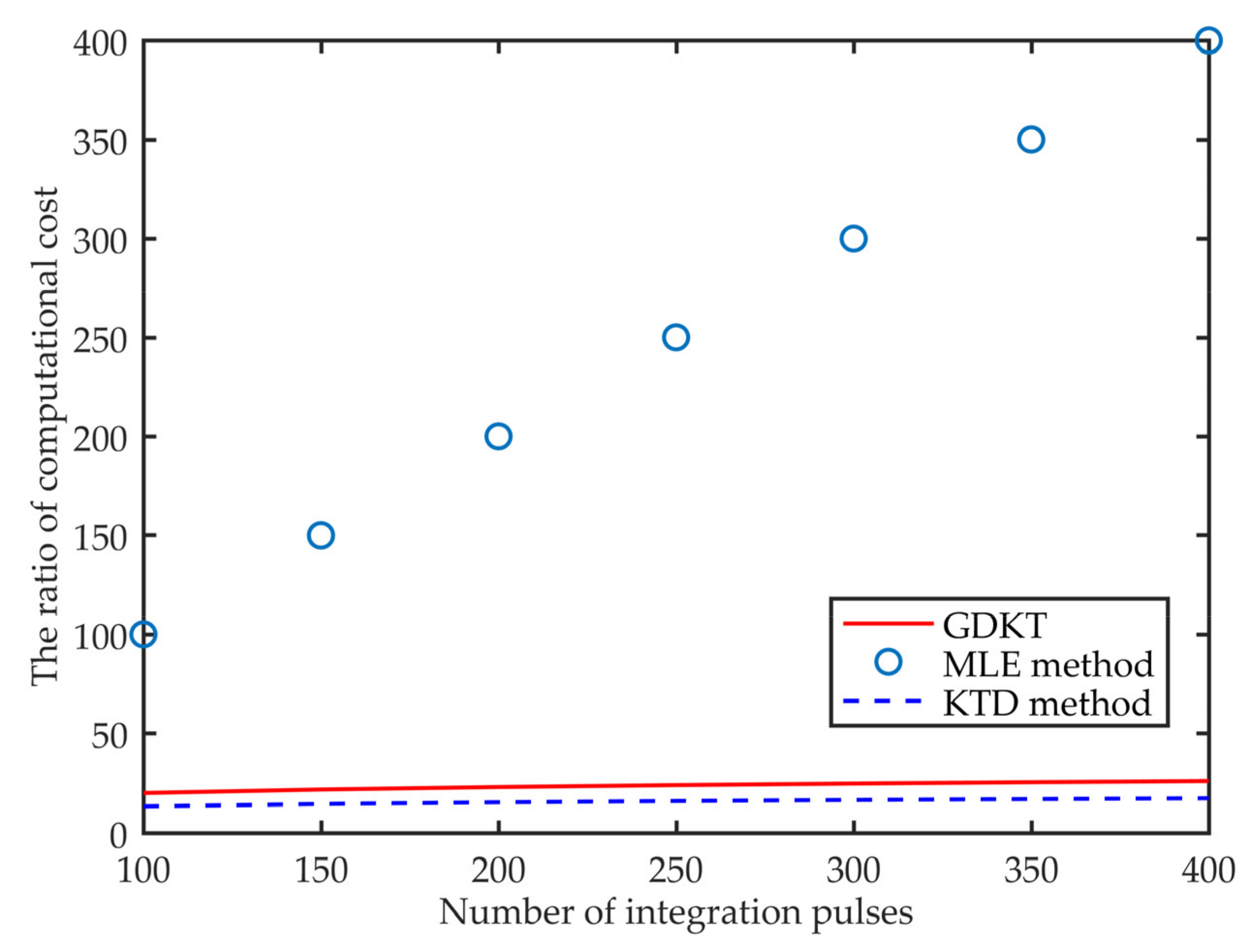
5.1. Computational Cost

In this subsection, we compare the computational cost of the GDKT to those of the MLE method and the KTD method. With the implementation method presented in SubSection 4.2, we obtain that the computational cost of the GDKT is in the order of $O\left[N_{{\widehat{N}}_{0d}}{N}_{{\widehat{a}}_1}\cdots N_{{\widehat{a}}_N}\left(2N_{f}M{\log }_{2}M+M{N}_f{\log }_2{N}_f\right)\right]$. Based on the implementation methods presented in [16] and [25], we obtain that computational costs of the KTD method and MLE method are in the order of $O\left[N_{{\widehat{N}}_{0d}}{N}_{{\widehat{a}}_1}\cdots N_{{\widehat{a}}_N}\left(N_{f}M{\log }_{2}M+M{N}_f{\log }_2{N}_f\right)\right]$ and $O\left[N_{{\widehat{f}}_0}{N}_{{\widehat{a}}_1}\cdots N_{{\widehat{a}}_N}{N}_{f}M\right]$, respectively (where $N_{{\widehat{f}}_0}$ denotes searching times for the unknown parameter $f_{k0}$). For easy comparison and without loss of generality, we assume $N_f=M$ [24,25,26,27] and obtain the ratio for computational costs of these three methods as

$$\frac{\frac{O\left[N_{{\widehat{N}}_{0d}}{N}_{{\widehat{a}}_1}\cdots N_{{\widehat{a}}_N}\left(2N_{f}M{\log }_{2}M+M{N}_f{\log }_2{N}_f\right)\right]}{O\left[N_{{\widehat{f}}_0}{N}_{{\widehat{a}}_1}\cdots N_{{\widehat{a}}_N}{N}_{f}M\right]}}{O\left[N_{{\widehat{N}}_{0d}}{N}_{{\widehat{a}}_1}\cdots N_{{\widehat{a}}_N}\left(N_{f}M{\log }_{2}M+M{N}_f{\log }_2{N}_f\right)\right]}\approx \frac{\frac{O\left[3N_{{\widehat{N}}_{0d}}{\log }_{2}M\right]}{O\left[N_{{\widehat{f}}_0}\right]}}{O\left[2N_{{\widehat{N}}_{0d}}{\log }_{2}M\right]}$$

(29)

$N_{{\widehat{f}}_0}$,$N_{{\widehat{N}}_{0d}}$ and ${\log }_{2}M$ determine the ratio in the Equation (29). Assume the searching range for unknown $v_{k0}$ is $\left[-v_{0\_\max },v_{0\_\max }\right]$. Based on $N_{{\widehat{f}}_0}\approx N_{{\widehat{N}}_{0d}}M$ [24,25,26,27], the ratio in Equation (29) can be rewritten as

$$\frac{\frac{O\left[3N_{{\widehat{N}}_{0d}}{\log }_{2}M\right]}{O\left[N_{{\widehat{f}}_0}\right]}}{O\left[2N_{{\widehat{N}}_{0d}}{\log }_{2}M\right]}\approx \frac{\frac{O\left[3{\log }_{2}M\right]}{O\left[M\right]}}{O\left[2{\log }_{2}M\right]}$$

(30)

Equation (30) indicates that computational costs of the GDKT and the KTD method are similar and much lower than that of the MLE method. In order to give a more intuitive comparison, Figure 6 shows the computational complexity ratio versus different numbers of integration pulses.

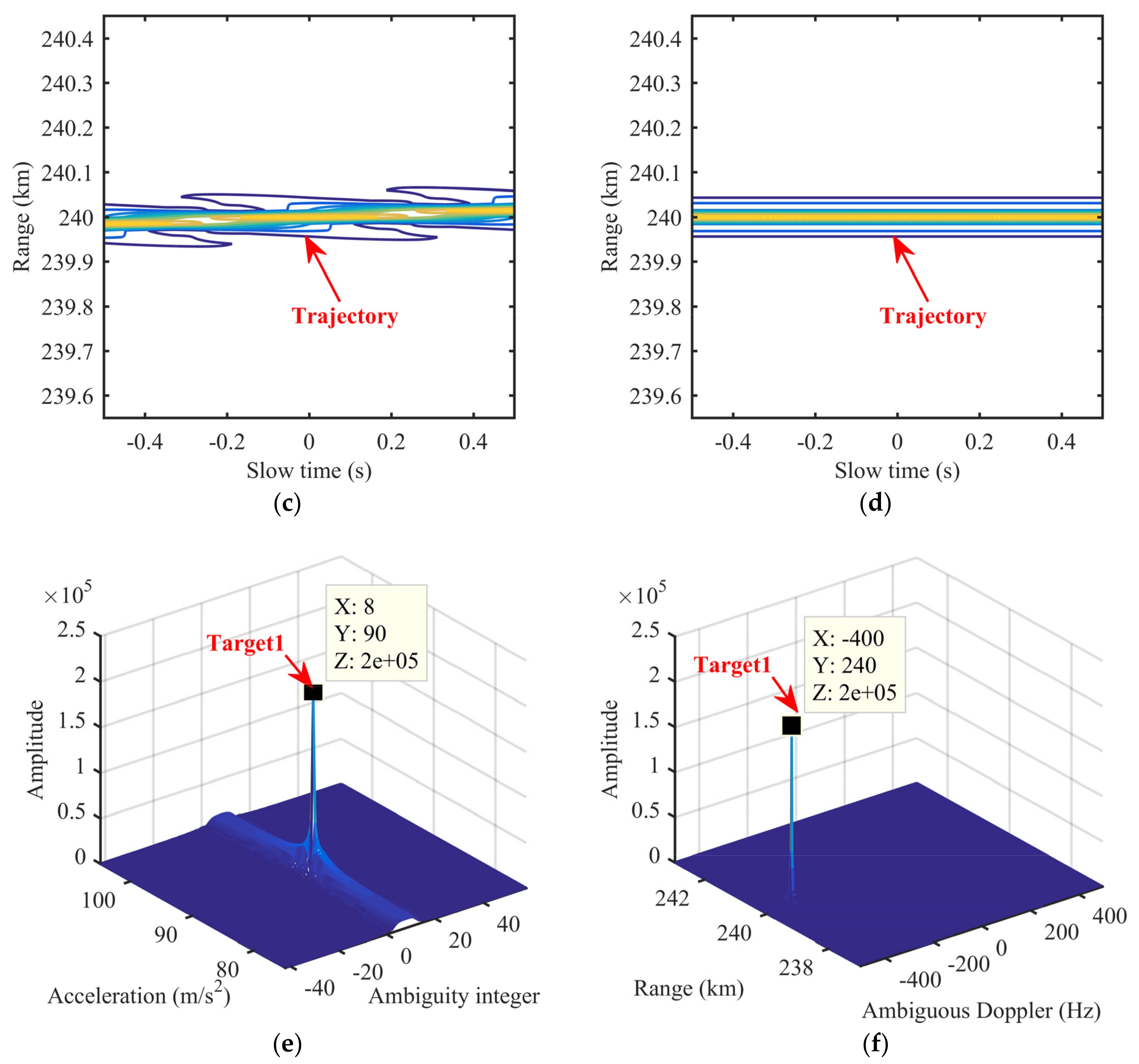
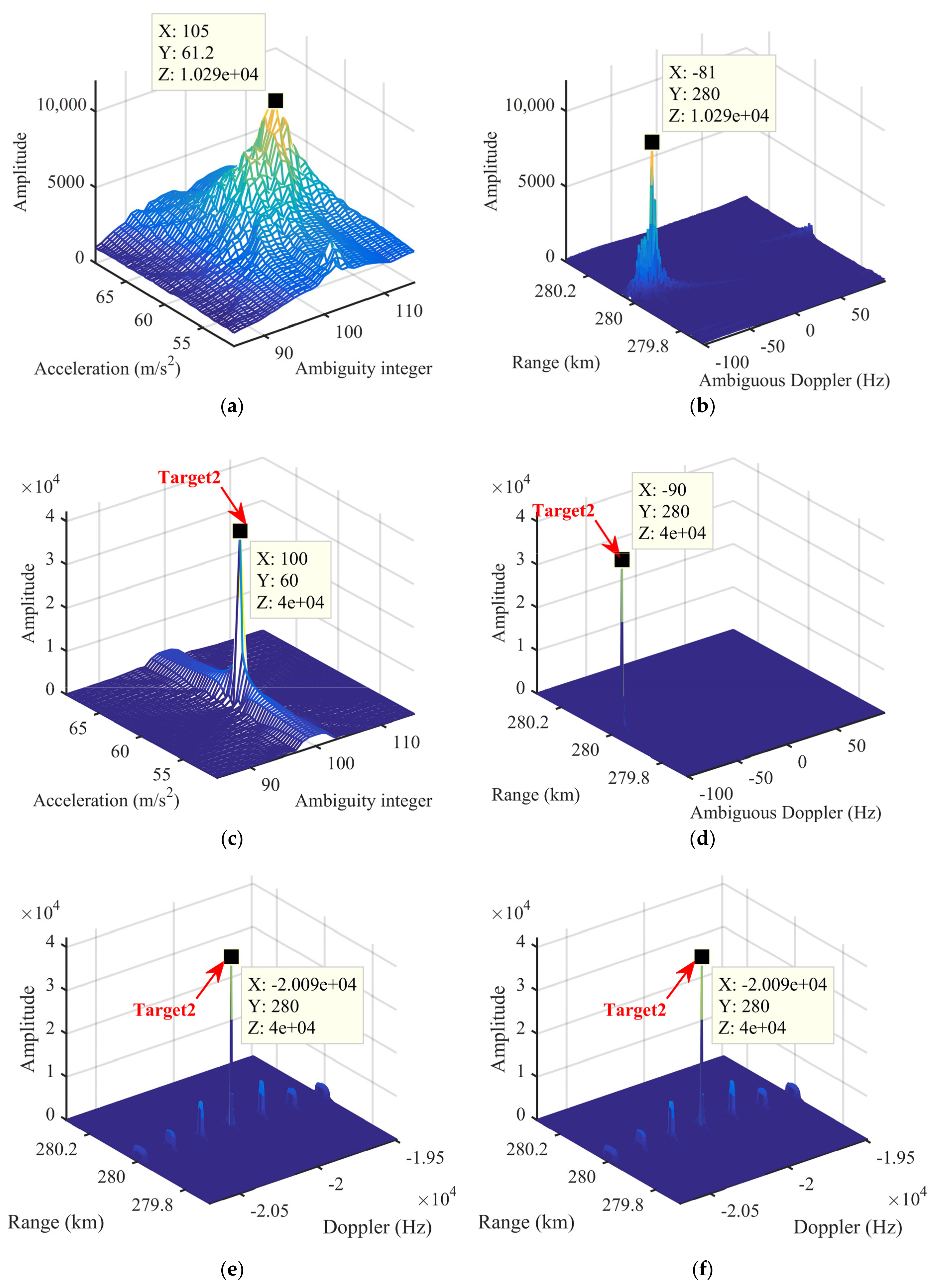
5.2. Energy Integration

In this subsection, we compare the energy integration of the MLE method, KTD method, and GDKT. The analyses above have indicated that due to the Doppler spectrum coupling and half-blind-velocity effect, the KTD method may encounter the defocusing of the energy integration. By contrast, the MLE method and GDKT do not encounter these two problems and could obtain the perfect energy integration. Here, we use an example to illustrate the energy integration of these three methods.

Example 4:

These three methods are linear. For the convenience of the image presentation and without loss of generality, we consider a uniformly accelerated target, i.e., Target2. The radar and target parameters are given in

Table 2. Radar and target parameters.

Radar Parameters
Carrier frequency		4 GHz		PRF			200 Hz
Bandwidth		100 MHz		Sampling frequency			200 MHz
Pulse width		1 μs		Number of pulses			200
Target Parameters
Target2	Backscattering coefficient		Range (km)		Velocity (m/s)	Acceleration (m/s2)
	1		140		753.375	60

. In this example, M is set to 200 to satisfy the deduced Equation (15). Figure 7 shows the simulation results of these three methods.

Figure 7a,b show the acceleration-ambiguity integer slice and range-ambiguous Doppler slice of the KTD method, respectively. Based on the radar and target parameters listed in Table 2, we separately analyze the Doppler spectrum coupling and half-blind-velocity effect in Equations (31) and (32) as

$$f_{k0d}+2f_{k1}{t}_m=90+1600t_m\Rightarrow -710\le f_{k0d}+2f_{k1}{t}_m\le 890$$

(31)

$$\frac{c}{f_c-B/2}\le \lambda \le \frac{c}{f_c+B/2}\Rightarrow 19838\le f_{k0}\le 20341$$

(32)

Equation (31) indicates that the Doppler spectrum coupling makes the Doppler spectrum span eight PRF bands. Equation (32) indicates that the half-blind-velocity effect makes the Doppler spectrum span three PRF bands. Therefore, the KTD method encounters the defocusing of the energy integration. By contrast, in the GDKT, the KT is employed after eliminating the influence of the Doppler spectrum coupling and half-blind-velocity effect. Therefore, same as the MLE method in Figure 7e,f, the GDKT in Figure 7c,d do not encounter the defocusing of the energy integration. Note that, although in this example, M is set to 200 to satisfy the deduced Equation (15), the BSSLs are still obvious in Figure 7e and may influence the weak targets’ detection and localization. Therefore, in the future, the BSSLs’ elimination method is still necessary.

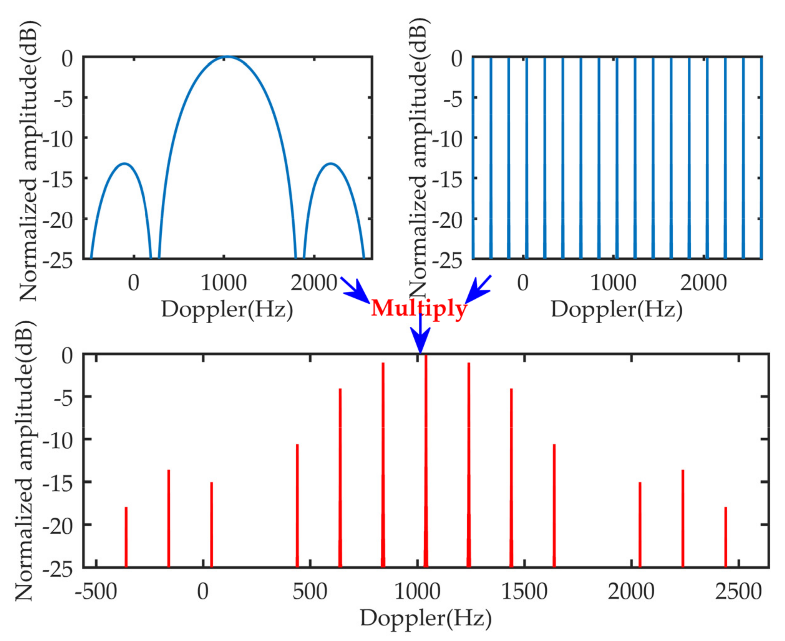
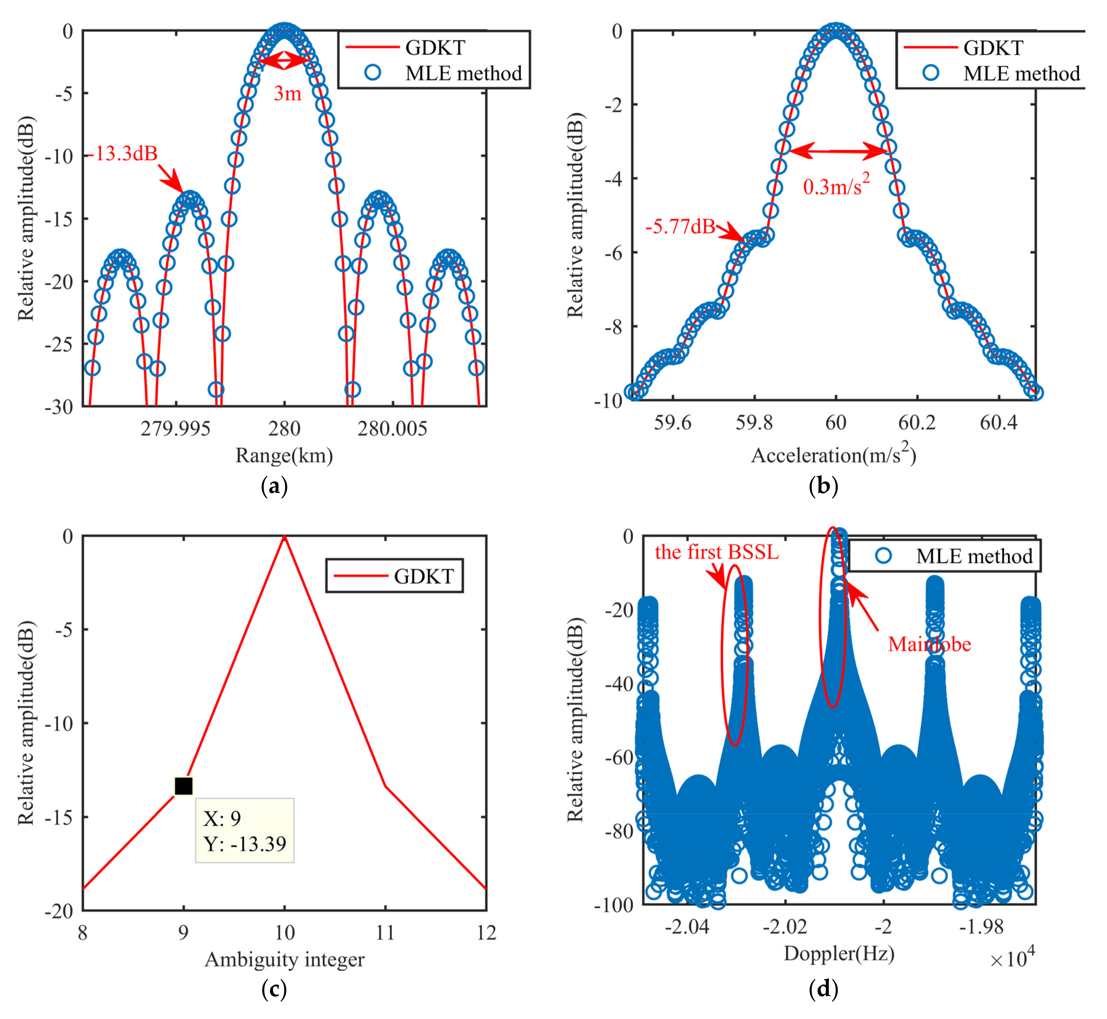
5.3. Resolution and PSL

The resolution and PSL play important roles in the adjacent targets’ detection and localization. The KTD method encounters the defocusing of the energy integration. Therefore, we only compare the GDKT with the MLE method. Based on the closed analytical formulae of the MLE method and GDKT in Equations (14) and (21), we present their theoretical resolutions and PSLs as

$$\left\{\begin{array}{l}{\delta }_{\mathrm{MLE}}\left({\widehat{R}}_0\right)={\delta }_{\mathrm{GDKT}}\left({\widehat{R}}_0\right)=\frac{c}{2B}\\ {\delta }_{\mathrm{MLE}}\left({\widehat{a}}_N\right)={\delta }_{\mathrm{GDKT}}\left({\widehat{a}}_N\right)=\frac{2^N\left(N+1\right)!c}{T_m^2{f}_c}\\ {\delta }_{\mathrm{MLE}}\left({\widehat{f}}_{0\_\mathrm{mainlobe}}\right)={\delta }_{\mathrm{GDKT}}\left({\widehat{f}}_{0d}\right)=\frac{1}{T_m}\\ \frac{{\delta }_{\mathrm{MLE}}\left({\widehat{f}}_{0\_outline}\right)}{\mathrm{PRF}}={\delta }_{\mathrm{GDKT}}\left({\widehat{N}}_{0d}\right)=\frac{3c}{B{T}_m\lambda \mathrm{PRF}}\end{array}\right.$$

(33)

$$\left\{\begin{array}{l}{\mathrm{PSL}}_{\mathrm{MLE}}\left({\widehat{R}}_0\right)={\mathrm{PSL}}_{\mathrm{GDKT}}\left({\widehat{R}}_0\right)=-13.3\mathrm{dB}\\ {\mathrm{PSL}}_{\mathrm{MLE}}\left({\widehat{a}}_N\right)={\mathrm{PSL}}_{\mathrm{GDKT}}\left({\widehat{a}}_N\right)=-13.3\mathrm{dB}\\ {\mathrm{PSL}}_{\mathrm{MLE}}\left({\widehat{f}}_{0\_\mathrm{mainlobe}}\right)={\mathrm{PSL}}_{\mathrm{GDKT}}\left({\widehat{f}}_{0d}\right)=-13.3\mathrm{dB}\\ {\mathrm{PSL}}_{\mathrm{MLE}}\left({\widehat{f}}_{0\_outline}\right)={\mathrm{PSL}}_{\mathrm{GDKT}}\left({\widehat{N}}_{0d}\right)=-13.3\mathrm{dB}\end{array}\right.$$

(34)

For the MLE method, we use ${\widehat{f}}_{0\_\mathrm{mainlobe}}$ and ${\widehat{f}}_{0\_\mathrm{outline}}$ to separately present the main lobe part and outline along the Doppler domain. Equations (33) and (34) indicate that theoretical resolutions and PSLs of the MLE method and GDKT are the same. Here, we use an example to illustrate the resolutions and PSLs of these two methods.

Example 5:

The radar and target parameters are the same as those listed in Table 2. Figure 8a shows simulation results along the range dimension. Figure 8b shows simulation results along the acceleration dimension. Figure 8c shows simulation results along the ambiguity integer dimension. Figure 8d shows the simulation results along the Doppler dimension. Figure 8e shows the simulation results along the ambiguous Doppler dimension. Figure 8f shows the zoom part of the first BSSL marked in Figure 8d.

With radar parameters and Equation (33), we could obtain that, for the MLE method and GDKT, theoretical resolutions along the range, ambiguous Doppler (or ${\widehat{f}}_{0\_\mathrm{mainlobe}}$) and acceleration should be 3 m, 1 Hz, and 0.3 m/s², respectively. Simulated resolutions in Figure 8 conform to theoretical resolutions. Simulated PSLs along the acceleration dimension is lower than the theoretical PSL given in Equation (34). This is because corresponding integration variables are different from those in the integrant and the sidelobe is elevated under the finite discrete signal [38,39]. The signal energy distribution along ${\widehat{N}}_{0d}$ can be seen as extractions of the ${\widehat{f}}_0$ dimension at ambiguity integers. When the extraction is just not the peak of the first BSSL, the influence of the BSSLs can be reduced. Figure 8f shows zoom part of the first BSSL marked in Figure 8d. Comparing Figure 8f to Figure 8c, we find that the extractions in the GDKT is not the peak of the first BSSL and the influence of the BSSLs is obviously reduced, which indicates that the GDKT benefits the PSL.

5.4. Anti-Noise Performance

This section focuses on the theoretical anti-noise performance analysis of the GDKT. The GDKT is linear. Without loss of generality, we consider the discrete noisy echo $s_e\left(n_{\widehat{t}},n_{t_m}\right)$ of the kth high-speed maneuvering target.

$$s_e\left(n_{\widehat{t}},n_{t_m}\right)=s_{s,e}\left(n_{\widehat{t}},n_{t_m}\right)+n_e\left(n_{\widehat{t}},n_{t_m}\right)$$

(35)

where $s_{s,e}\left(n_{\widehat{t}},n_{t_m}\right)$ denotes the discrete echo of the kth target. $n_e\left(n_{\widehat{t}},n_{t_m}\right)$ denotes the discrete noise.

Via the Fourier transform along the fast time dimension of $s_e\left(n_{\widehat{t}},n_{t_m}\right)$, we obtain the discrete noisy echo in the slow time-range frequency domain.

$$S_e\left(n_f,n_{t_m}\right)=S_{s,e}\left(n_f,n_{t_m}\right)+n_{S,e}\left(n_f,n_{t_m}\right)$$

(36)

Now, we use $S_{trans}\left(n_f\right)$ (the transmitting waveform in the range frequency domain) to perform the range compression, and then perform the GDKT.

$$\begin{array}{l}\mathrm{GDKT}\left(n_{\widehat{t}},n_{f_{t_m}},{\widehat{N}}_{0d},n_{{\widehat{a}}_1},\cdots ,n_{{\widehat{a}}_N}\right)={\displaystyle \sum _{n_f}{\displaystyle \sum _{n_{t_m}}{S}_e\left(n_f,n_{t_m}\right)S_{trans}^{*}\left(n_f\right)}}\\ \times \exp \left(j2\pi \frac{n_f{\Delta }_f}{c}\lambda {\widehat{N}}_{0d}\mathrm{PRF}{n}_{t_m}{\Delta }_{t_m}\right)\exp \left(j2\pi \frac{n_{f_{t_m}}}{M}\frac{n_f{\Delta }_f+f_c}{f_c}{n}_{t_m}\right)\\ \times \exp \left\{j4\pi \frac{n_f{\Delta }_f+f_c}{c}\left[\frac{n_{{\widehat{a}}_1}{\Delta }_{{\widehat{a}}_1}}{2}{\left(n_{t_m}{\Delta }_{t_m}\right)}^2+\cdots +\frac{n_{{\widehat{a}}_N}{\Delta }_{{\widehat{a}}_N}}{\left(N+1\right)!}{\left(n_{t_m}{\Delta }_{t_m}\right)}^{N+1}\right]\right\}\\ \times \exp \left(j2\pi n_f{\Delta }_f{n}_{\widehat{t}}{\Delta }_{\widehat{t}}\right)\end{array}$$

(37)

where * denotes the complex conjugation. ${\Delta }_{\widehat{t}}$ denotes the range sampling interval.

In order to analyze the theoretical detection and localization performance, we use the software “Wolfram Mathematica” and properties of the moment of zero mean complex Gaussian random variables to calculate the expect value at the peak point.

$$E\left[{\left|\mathrm{GDKT}\left(n_{R_{k0}},n_{f_{k0d}},N_{0d},n_{a_1},\cdots ,n_{a_N}\right)\right|}^2\right]={\left(B{T}_p{T}_m\mathrm{PRF}\right)}^2{A}_k^2+\left(B{T}_p{T}_m\mathrm{PRF}\right){\sigma }_n^2$$

(38)

where $\left(n_{R_{k0}},n_{f_{k0d}},N_{0d},n_{a_1},\cdots ,n_{a_N}\right)$ corresponds to the discrete points of $\left(R_{k0},v_{k0},f_{k0d},a_{k1},\cdots ,a_{kN}\right)$.

The output SNR after the GDKT is

$${\rho }_{\mathrm{GDKT}}=B{T}_p{T}_m\mathrm{PRF}\frac{A_k^2}{{\sigma }_n^2}=B{T}_p{T}_m\mathrm{PRF}{\rho }_k$$

(39)

Equations (8) and (39) indicate that, same as the MLE method [16,17], the anti-noise performance of GDKT is statically optimal. In this subsection, we use a numerical example to validate analyses of the theoretical anti-noise performance.

Example 6:

The radar and target parameters are the same as those in Table 2. The simulated radar data is contaminated by the zero-mean white Gaussian noise and the input SNRs are set as [−40:1: 10] dB. 1000 trials are done for each input SNR value. Figure 9a–c shows the detection probabilities under the false alarm rates 10⁻⁵, 10⁻⁶, and 10⁻⁷, respectively. The MLE method, KTD method, and MTD method are used as comparisons.

Due to the RCM and DFM, the MTD has a bad anti-noise performance in Figure 9. As analyzed above, the Doppler spectrum coupling and half-blind-velocity effect influence the anti-noise performance of the KTD method seriously. Figure 9 shows that the anti-noise performance of the KTD is about 13 dB worse than those of the GDKT and the MLE method. On the contrary, the GDKT can compensate the RCM and DFM without the anti-noise performance loss. Therefore, under false alarm rates 10⁻⁵, 10⁻⁶, and 10⁻⁷, its detection probabilities are almost the same as those of the MLE method, which conforms to the theoretical anti-noise performance analyses.

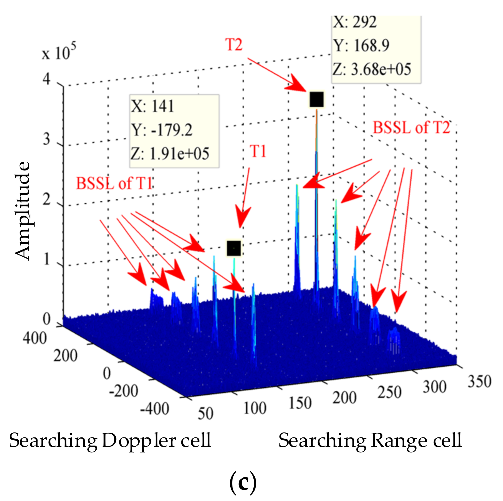
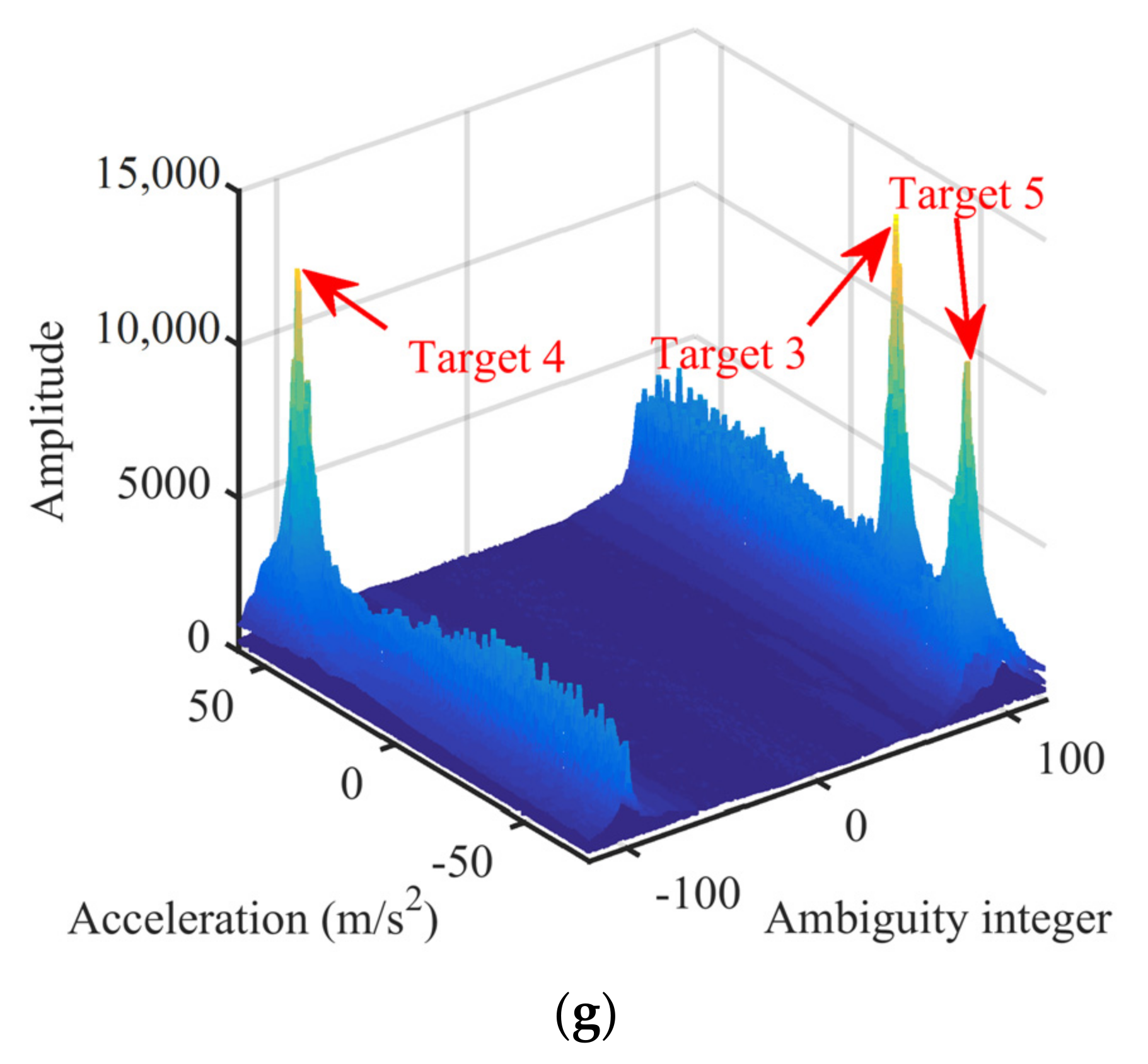
5.5. Practicability under Multicomponent High-Speed Maneuvering Targets

The analyses above indicate that considering the computational cost, energy integration, resolution, PSL, and anti-noise performance, the GDKT is more suitable for the high-speed maneuvering target detection and localization than other methods. In this subsection, we use a numerical example to demonstrate the practicability of the GDKT under multi-component high-speed maneuvering targets. The MTD method, MLE method, and KTD method are used for comparisons.

Example 7:

These four methods are all linear. Therefore, for the convenience of the image presentation and the clear comparison, we consider three uniformly accelerated targets, i.e., Target3, Target4, and Target5, without noise. The target parameters are listed in

Table 3. Target Parameters.

-	Backscattering Coefficient	Range (km)	Velocity (m/s)	Acceleration (m/s2)
Target3	1	129.97	738.375	−30
Target4	1	130.015	−738	48
Target5	1	130.03	662.625	−63

and radar parameters are the same as those in Table 2. Figure 10 shows the simulation results.

Figure 10a shows the integration result of the MTD method. The RCM and DFM occur and the echo energy cannot be integrated via the MTD method. Figure 10b,c show the range-ambiguous Doppler slice and acceleration-ambiguity integer slice of the GDKT, respectively. The GDKT eliminates the RCM and DFM completely and completes the echo energy integration. Figure 10d,e show the range-Doppler slice and acceleration dimension of the MLE method, respectively. As expected, the MLE method also eliminates the RCM and DFM completely and completes the echo energy integration. Figure 10f,g show the range-ambiguous Doppler slice and acceleration- ambiguity integer slice of the KTD method, respectively. Based on the radar parameters, motion parameters, and Equations (31) and (32), we could obtain that the Doppler spectrum coupling and half-blind-velocity effect make the Doppler spectrum of these three targets span several PRF bands. Therefore, the KTD method encounters the defocusing of the energy integration in Figure 10f,g. Combined with the computational cost analysis, we can say that the GDKT is more suitable for radar high-speed maneuvering target detection and localization than the MLE method and KTD method.

Here, based on mathematical analyses and numerical simulations, we provide a final table (see

Table 4. Performance comparisons.

-	Computational Cost	Detection and Localization Performance	Practicability
MTD	low	low	low
MLE	high	high	low
KTD	low	low	low
GDKT	low	high	high

) comparing the performances of the MTD method, MLE method, KTD method, and GDKT. From this table, it is very easy to find that the GDKT is more suitable for radar high-speed maneuvering target detection and localization.

6. Real Radar Data Validation

In this section, we use the real radar data to validate the proposed detection and localization method. As we know, due to the complicated and unknown realistic environment, it is difficult to control the SNR and radial motion parameters. Therefore, in this paper, we only use the real radar data to validate the practicability of the GDKT instead of its superiorities. All processing of the real radar data is completed on a personal computer with an Intel (R) Xeon (R) CPU E5-1603 v4(3.70 GHz) processor and 64 GB memory.

The raw data were recorded by an X-band ground-based radar. This radar transmits the LFMCW waveform with the PRF of 50 Hz and a bandwidth of 500 MHz. In the following simulations, 216 effective pulses are extracted from the data set. Figure 11a shows the experiment scene and Figure 11b shows trajectories after the range compression. The GDKT takes the ambiguity integer searching into consideration. When the ambiguity integer is found correctly, the target energy can be integrated as much as possible in the range- ambiguous Doppler slice. Figure 11c shows the energy integration result when the ambiguity integer, k = 3, is correctly compensated in the range- ambiguous Doppler slice. To observe the effect of ambiguity number compensation on the energy integration, the energy focusing result in the ambiguous Doppler-ambiguity integer slice with the range gate number 455 is shown in Figure 11d. Obviously, if the ambiguity integer is not compensated correctly, the energy integration effect will become worse as the searching parameter is far away from the correct value. In order to show the superiority of the GDKT in the energy integration effect, the energy integration effect of the MTD algorithm is shown in Figure 11e. Because there is no correction of the RCM, the energy is scattered in different range units and the integration effect of MTD is very poor.

7. Conclusions and Future Work

For radar high-speed maneuvering target detection and localization, this paper names two signal processing modes, i.e., PU mode and PS mode, and then deduces closed analytical formulae of two typical methods, i.e., the MLE method and the KTD method, for a better understanding of these two modes. With the deduced closed analytical formulae, we interpret several doubts in radar high-speed maneuvering target detection and localization, such as the BSSL and the relationship between the PU and PS modes. Thereafter, based on the principle of the PS mode, the GDKT is proposed for radar high-speed maneuvering target detection and localization. Mathematical analyses and numerical simulations are used to demonstrate that the GDKT has a statistically optimal anti-noise performance and is computational efficiently.

We think that the largest significance of this paper is the interpretation of the PU and PS modes. Although the GDKT is statically optimal and computationally efficient, its computational cost is still a little high. Therefore, in the future, we will continue to study the PS mode and fast implementation of the GDKT. In addition, the resolution enhancement via the compressed sensing and the BSSL suppression method will also be studied [40,41]. Other signal waveforms, i.e., nonlinear LFM signal waveform, can also be used [42].

References

1. Moses, P.L.; Rausch, V.L.; Nguyen, L.T.; Hill, J.R. NASA hypersonic flight demonstrators—Overview, status, and future plans. Acta Astronaut. 2004, 55, 619–630. [Google Scholar] [CrossRef]
2. De Miao, A.; Farina, A.; Gertach, K. Adaptive detection of range spread targets with orthogonal rejection. IEEE Trans. Aerosp. Electron. Syst. 1999, 47, 1522–1531. [Google Scholar]
3. Gini, F.; Greco, M.; Farina, A. Clairvoyant and adaptive signal detection in non-Gaussian clutter: A data-dependent threshold interpretation. IEEE Trans. Signal Process. 2012, 60, 6190–6201. [Google Scholar] [CrossRef]
4. Orlando, D.; Frank, E.; Giuseppe, R. Track-before-detect algorithms for bistatic sonars. In Proceedings of the 2010 2nd IEEE International Workshop on Cognitive Information Processing, Elba, Italy, 14–16 June 2010; pp. 180–185. [Google Scholar]
5. Jia, X.; Peng, Y.N.; Xia, X.G.; Farina, A. Focus-before-detection radar signal processing: Part i—Challenges and methods. IEEE Aerosp. Electron. Syst. Mag. 2017, 32, 48–59. [Google Scholar]
6. Jia, X.; Peng, Y.N.; Xia, X.G.; Long, T.; Mao, E.-K. Focus-before-detection radar signal processing: Part ii—Recent developments. IEEE Aerosp. Electron. Syst. Mag. 2018, 33, 34–49. [Google Scholar]
7. Ehlers, F.; Orlando, D.; Ricci, G. Batch tracking algorithm for multistatic sonars. IET Radar Sonar Navig. 2012, 6, 746–752. [Google Scholar] [CrossRef]
8. Jin, K.; Li, G.; Lai, T.; Jin, T.; Zhao, Y. A Novel Long-Time Coherent Integration Algorithm for Doppler-Ambiguous Radar Maneuvering Target Detection. IEEE Sens. J. 2020, 20, 9394–9407. [Google Scholar] [CrossRef]
9. Sun, Z.; Li, X.; Cui, G.; Yi, W.; Kong, L. Hypersonic Target Detection and Velocity Estimation in Coherent Radar System Based on Scaled Radon Fourier Transform. IEEE Trans. Veh. Technol. 2020, 69, 6525–6540. [Google Scholar] [CrossRef]
10. Carlson, B.; Evans, E.; Wilson, S. Search radar detection and track with the Hough transform. I. system concept. IEEE Trans. Aerosp. Electron. Syst. 1994, 30, 102–108. [Google Scholar] [CrossRef]
11. Carlson, B.; Evans, E.; Wilson, S. Search radar detection and track with the Hough transform. II. Detection statistics. IEEE Trans. Aerosp. Electron. Syst. 1994, 30, 109–115. [Google Scholar] [CrossRef]
12. Carlson, B.D.; Evans, E.D.; Wilson, S.L. Search radar detection and track with the Hough transform. III. Detection performance with binary integration. IEEE Trans. Aerosp. Electron. Syst. 1994, 30, 116–125. [Google Scholar] [CrossRef]
13. Carretero-Moya, J.; Gismero-Menoyo, J.; Asensio-Lopez, A.; Blanco-del-Campo, A. Application of the radon transform to detect small-targets in sea clutter. IET Radar Sonar Navig. 2009, 3, 155–166. [Google Scholar] [CrossRef]
14. Copeland, A.C.; Ravichandran, G.; Trivedi, M.M. Localized Radon transform-based detection of ship wakes in SAR images. IEEE Trans. Geosci. Remote. Sens. 1995, 33, 35–45. [Google Scholar] [CrossRef]
15. Tandra, R.; Sahai, A. SNR walls for signal detection. IEEE J. Sel. Top. Signal Process. 2008, 2, 4–17. [Google Scholar] [CrossRef] [Green Version]
16. Abatzoglou, T.J.; Gheen, G.O. Range, radial velocity, and acceleration MLE using radar LFM pulse train. IEEE Trans. Aerosp. Electron. Syst. 1998, 34, 1070–1083. [Google Scholar] [CrossRef]
17. Xu, J.; Xia, X.-G.; Peng, S.-B.; Yu, J.; Peng, Y.-N.; Qian, L.-C. Radar maneuvering target motion estimation based on generalized Radon-Fourier transform. IEEE Trans. Signal Process. 2012, 60, 6190–6201. [Google Scholar]
18. Chen, X.; Guan, J.; Liu, N.; He, Y. Maneuvering target detection via Radon-fractional Fourier transform-based long-time coherent integration. IEEE Trans. Signal Process. 2014, 62, 939–953. [Google Scholar] [CrossRef]
19. Wu, W.; Wang, G.H.; Sun, J.P. Polynomial Radon-polynomial Fourier transform for near space hypersonic maneuvering target detection. IEEE Trans. Aerosp. Electron. Syst. 2017, 54, 1306–1322. [Google Scholar] [CrossRef]
20. Perry, R.; Dipietro, R.; Fante, R. SAR imaging of moving targets. IEEE Trans. Aerosp. Electron. Syst. 1999, 35, 188–200. [Google Scholar] [CrossRef]
21. Wang, C.; Jiu, B.; Liu, H. Maneuvering target detection in random pulse repetition interval radar via resampling-keystone transform. Signal Process. 2021, 181, 107899. [Google Scholar] [CrossRef]
22. Fang, X.; Xiao, G.; Cao, Z.; Min, R.; Pi, Y. Migration Correction Algorithm for Coherent Integration of Low-Observable Target With Uniform Radial Acceleration. IEEE Trans. Instrum. Meas. 2020, 70, 1–13. [Google Scholar] [CrossRef]
23. Zheng, J.; Yang, T.; Liu, H.; Su, T.; Wan, L. Accurate detection and localization of UAV swarms-enabled MEC system. IEEE Trans. Ind. Inform. 2020, 17, 5059–5067. [Google Scholar] [CrossRef]
24. Zheng, J.; Chen, R.; Yang, T.; Liu, X.; Liu, H.; Su, T.; Wan, L. An efficient strategy for accurate detection and localization of UAV swarms. IEEE Internet Things J. 2021. [Google Scholar] [CrossRef]
25. Kong, L.; Li, X.; Cui, G.; Yi, W.; Yang, Y. Coherent integration algorithm for a maneuvering target with high-order range migration. IEEE Trans. Signal Process. 2015, 63, 4474–4486. [Google Scholar] [CrossRef]
26. Huang, P.; Liao, G.; Yang, Z.; Xia, X.-G.; Ma, J.-T.; Ma, J. Long-time coherent integration for weak maneuvering target detection and high-order motion parameter estimation based on keystone transform. IEEE Trans. Signal Process. 2016, 64, 4013–4026. [Google Scholar] [CrossRef]
27. Sun, G.; Xing, M.; Xia, X.-G.; Wu, Y.; Bao, Z. Robust ground moving-target imaging using deramp–keystone processing. IEEE Trans. Geosci. Remote. Sens. 2012, 51, 966–982. [Google Scholar] [CrossRef]
28. Kirkland, D. Imaging moving targets using the second-order keystone transform. IET Radar Sonar Navig. 2011, 5, 902–910. [Google Scholar] [CrossRef]
29. Scott, K.M.; Barott, W.C.; Himed, B. The keystone transform: Practical limits and extension to second order corrections. In Proceedings of the 2015 IEEE Radar Conference (RadarCon), Arlington, VA, USA, 10–15 May 2015; pp. 1264–1269. [Google Scholar]
30. Xu, J.; Zhou, X.; Qian, L.-C.; Xia, X.-G.; Long, T. Hybrid integration for highly maneuvering radar target detection based on generalized Radon-Fourier transform. IEEE Trans. Aerosp. Electron. Syst. 2016, 52, 2554–2561. [Google Scholar] [CrossRef]
31. Jin, K.; Lai, T.; Wang, Y.; Li, G.; Zhao, Y. Radar coherent detection for Doppler-ambiguous maneuvering target based on product scaled periodic Lv’s distribution. Signal Process. 2020, 174, 107617. [Google Scholar] [CrossRef]
32. Li, X.; Cui, G.; Kong, L.; Yi, W. Fast non-searching method for maneuvering target detection and motion parameters estimation. IEEE Trans. Signal Process. 2016, 64, 2232–2244. [Google Scholar] [CrossRef]
33. Li, X.; Cui, G.; Yi, W.; Kong, L. Radar maneuvering target detection and motion parameter estimation based on TRT-SGRFT. Signal Process. 2017, 133, 107–116. [Google Scholar] [CrossRef]
34. Jin, K.; Lai, T.; Wang, Y.; Xing, X.; Zhao, Y. Parameter estimation of quadratic frequency modulated signal based on three-dimensional scaled Fourier transform. IET Radar Sonar Navig. 2019, 13, 1689–1696. [Google Scholar] [CrossRef]
35. Zheng, J.; Liu, H.; Liu, J.; Du, X.; Liu, Q.H. Radar high-speed maneuvering target detection based on three-dimensional scaled transform. IEEE J. Sel. Top. Appl. Earth Obs. Remote. Sens. 2018, 11, 2821–2833. [Google Scholar] [CrossRef]
36. Yu, J.; Xu, J.; Peng, Y.-N.; Xia, X.-G. Radon-Fourier transform for radar target detection (III): Optimality and fast implementations. IEEE Trans. Aerosp. Electron. Syst. 2012, 48, 991–1004. [Google Scholar] [CrossRef]
37. Xu, J.; Yu, J.; Peng, Y.-N.; Xia, X.-G. Radon-Fourier transform for radar target detection (II): Blind speed sidelobe suppression. IEEE Trans. Aerosp. Electron. Syst. 2011, 47, 2473–2489. [Google Scholar] [CrossRef]
38. Zheng, J.; Liu, H.; Liu, Q.H. Parameterized centroid frequency-chirp rate distribution for LFM signal analysis and mechanisms of constant delay introduction. IEEE Trans. Signal Process. 2017, 65, 6435–6447. [Google Scholar] [CrossRef]
39. Wang, Y.; Huang, X.; Zhang, Q. Rotation parameters estimation and cross-range scaling research for range instantaneous Doppler ISAR images. IEEE Sens. J. 2020, 20, 7010–7020. [Google Scholar] [CrossRef]
40. Niu, Z.; Zheng, J.; Su, T.; Li, W.; Zhang, L. Radar High-speed Target Detection Based on Improved Minimalized Windowed RFT. IEEE J. Sel. Top. Appl. Earth Obs. Remote. Sens. 2020, 14, 870–886. [Google Scholar] [CrossRef]
41. Park, Y.; Meyer, F.; Gerstoft, P. Sparse Bayesian learning for time-varying DOA estimation. J. Acoust. Soc. Am. 2020, 148, 2543. [Google Scholar] [CrossRef]
42. Jin, G.; Deng, Y.; Wang, R.; Wang, W.; Wang, P.; Long, Y.; Zhang, Z.; Zhang, Y. An advanced nonlinear frequency modulation waveform for radar imaging with low sidelobe. IEEE Trans. Geosci. Remote. Sens. 2019, 57, 6155–6168. [Google Scholar] [CrossRef]
Figure 1. Phenomenon of RCM, DFM and BSSL. (a) Phenomenon of RCM. (b) Phenomenon of DFM. (c) Phenomenon of BSSL.
Remotesensing 13 03367 g001aRemotesensing 13 03367 g001b
Figure 2. Illustration of the f ^ 0 dimension of Equation (14).
Remotesensing 13 03367 g002
Figure 3. Illustration of the N ^ 0 d and f ^ 0 d dimensions of Equation (19).
Remotesensing 13 03367 g003
Figure 4. Flow chart of GDKT method.
Remotesensing 13 03367 g004
Figure 5. Illustration of how the GDKT works. (a) Trajectory in the range-slow time domain after the pulse compression. (b) Integration result after performing the Fourier transform along the slow time dimension of (a), i.e., integration result of the MTD method. (c) Trajectory in the range-slow time domain after the dechirp operation of Step 2. (d) Trajectory in the range-slow time domain after the KT operation of Step 3. (e) Acceleration-ambiguity integer slice of the GDKT. (f) Range-ambiguous Doppler slice of the GDKT.
Remotesensing 13 03367 g005aRemotesensing 13 03367 g005b
Figure 6. Computational complexity ratio versus different integration pulses.
Remotesensing 13 03367 g006
Figure 7. Energy integration result. (a) Acceleration-ambiguity integer slice of the KTD method. (b) Range-ambiguous Doppler slice of the KTD method. (c) Acceleration-ambiguity integer slice of the GDKT. (d) Range-ambiguous Doppler slice of the GDKT. (e) Range-Doppler slice of the MLE method. (f) Acceleration dimension of the MLE method.
Remotesensing 13 03367 g007
Figure 8. Resolution and PSL. (a) Resolution and PSL along the range dimension. (b) Resolution and PSL along the acceleration dimension. (c) Resolution and PSL along the ambiguity integer dimension. (d) Resolution and PSL along the Doppler dimension. (e) Resolution and PSL along the ambiguous Doppler dimension. (f) Zoom part of the first BSSL marked in (d).
Remotesensing 13 03367 g008aRemotesensing 13 03367 g008b
Figure 9. Detection probability. (a) Detection probability under 10−5. (b) Detection probability under 10−6. (c) Detection probability under 10−7.
Remotesensing 13 03367 g009aRemotesensing 13 03367 g009b
Figure 10. Simulation results of Example 7. (a) Integration result of the MTD method. (b) Range-ambiguous Doppler slice of the GDKT. (c) Acceleration-ambiguity integer slice of the GDKT. (d) Range-Doppler slice of the MLE method. (e) Acceleration dimension of the MLE method. (f) Range-ambiguous Doppler slice of the KTD method. (g) Acceleration-ambiguity integer slice of the KTD method.
Remotesensing 13 03367 g010aRemotesensing 13 03367 g010b
Figure 11. Experiment scene and real radar data processing results. (a) Experiment scene. (b) Result of range compression. (c) Range-ambiguous Doppler slice of the GDKT. (d) Ambiguous Doppler-ambiguity integer slice of the GDKT. (e) Integration result of the MTD method.
Remotesensing 13 03367 g011