Two-Stream Convolutional Long- and Short-Term Memory Model Using Perceptual Loss for Sequence-to-Sequence Arctic Sea Ice Prediction

Abstract

Arctic sea ice plays a significant role in climate systems, and its prediction is important for coping with global warming. Artificial intelligence (AI) has gained recent attention in various disciplines with the increasing use of big data. In recent years, the use of AI-based sea ice prediction, along with conventional prediction models, has drawn attention. This study proposes a new deep learning (DL)-based Arctic sea ice prediction model with a new perceptual loss function to improve both statistical and visual accuracy. The proposed DL model learned spatiotemporal characteristics of Arctic sea ice for sequence-to-sequence predictions. The convolutional neural network-based perceptual loss function successfully captured unique sea ice patterns, and the widely used loss functions could not use various feature maps. Furthermore, the input variables that are essential to accurately predict Arctic sea ice using various combinations of input variables were identified. The proposed approaches produced statistical outcomes with better accuracy and qualitative agreements with the observed data.

1. Introduction

Sea ice, referred to as frozen seawater, is a primary indicator of global warming and climate change because of the ice–albedo feedback—open water absorbs solar energy, while sea ice reflects it [1]. Arctic sea ice also plays an essential role in climate change in mid-latitude regions [2]. Satellite observations using passive microwave sensors over a period of > 40 years have shown the long-term decline of Arctic sea ice, particularly in the last decade. The average sea ice is becoming younger, and multi-year ice regions at the beginning of the satellite record were greater than the first-year ice regions [3,4].

Owing to the importance of the role of Arctic sea ice in climate change and the Northern Sea Route for ship navigation, various studies were conducted to predict its properties, such as concentration, extent, motion, and thickness. Since 2008, researchers have reported on the September minimum sea ice extent (SIE) from various perspectives and have predicted it for the months of June, July, and August [5]. Most of these contributions were based on the results obtained using conventional statistical and numerical models in the past years, but results from machine learning-based models have recently been added.

The decreasing and thinning of ice are closely related to positive climate feedback leading to Arctic amplification [6,7]. Mioduszewski et al. [8] showed that ice area variability would grow substantially but not monotonically every month, based on many climate models. The changes in interannual variability in sea ice coverage have been studied only in a limited capacity, and irregular variability makes it challenging to predict Arctic sea ice concentration (SIC) and SIE. Therefore, owing to climate change, unpredictable and extreme anomalies are observed more frequently in the Arctic region.

Statistical prediction models exploit historical observations and relations between atmospheric, oceanic, and ice-related variables such as air temperature, sea-level pressure, sea-surface temperature, and the concentration, extent, type, and thickness of sea ice [9,10]. Numerical models use physical equations based on the atmosphere-ice-ocean interaction [11,12]. Artificial intelligence (AI) and deep learning (DL) techniques have been widely used for the prediction of sea ice characteristics. A special type of AI and an extension of neural networks have been applied for such predictions since 2017. Chi and Kim [13] conducted the first sea ice prediction study using DL approaches. They used only historical monthly sea ice concentration (SIC) data as input for the DL networks and produced results that were comparable to various statistical and numerical models for September predictions reported in the Sea Ice Outlook. Although the proposed long- and short-term memory (LSTM) model showed good predictability for the one-month prediction, it was inadequate for multistep predictions. Kim et al. [14] employed a DL method with a multimodel ensemble to provide a near-future prediction for the 10–20 forthcoming years. The proposed model determines the nonlinear relationship between sea ice and climate variables. Choi et al. [15] used a gated recurrent unit, a type of recursive neural network, to provide 15-day predictions. They used the spatial information of sea ice extent and SIC as input variables and compared the proposed model to that of the LSTM. These studies [13,14,15] were based on one-dimensional vector data; however, Choi et al. incorporated the image coordinates into the input vector data [12]. Kim et al. [16] proposed the convolutional neural network (CNN)–based models by incorporating various sea ice, atmospheric, and oceanic variables to provide one-month predictions. Although they exploited the spatial characteristics of sea ice data via CNN architectures, they trained 12 individual CNN models for the prediction of each month, which may be redundant. Liu et al. [17] used the convolutional LSTM (ConvLSTM) to predict daily Arctic SIC. Their proposed model outperformed the CNN-based model, particularly in simulating the local variations in the Northeast Passage, but it was designed for one-step predictions. Overall, current sea ice prediction models using DL approaches are limited to one-dimensional vector-based recurrent networks, CNN models without considering sequence information or conventional ConvLSTM.

To address the limitations of the current prediction models, we propose an ensemble model with a new loss function that enables multi-step Arctic sea ice predictions. Three primary goals are discussed. First, we propose a ConvLSTM model with different modalities to capture the spatiotemporal characteristics of historical sea ice information. Second, we introduce a new feature-based loss function to produce better qualitative prediction maps by comparing their perceptual characteristics. As addressed by us and others in previous studies [13,14,15,16], ice, atmospheric, and oceanic variables may be helpful in improving predictability. Finally, we test the significances of several input variables through the direct training of the model without using relative sensitivity tests.

2. Datasets

Conventional numerical, statistical, or ensemble models for sea ice prediction often use various ice-, ocean-, and atmosphere-related properties as input variables [9,11,12]. Based on previous DL-based sea ice prediction studies [13,14,15,16], we also used several sea ice and atmosphere-related variables. The details of the variables are provided in

Table 1. Details of input variables used in the Arctic sea ice prediction model.

Group	Variable	Abbreviation	Unit
Sea ice	Sea ice concentration	SIC	%
	Sea ice concentration anomaly	SICano	%
	Sea ice extent	SIE	Binary
ERA5	2 m temperature	T2m	K
	10 m V wind component	V10m	m/s
	10 m U wind component	U10m	m/s

.

2.1. Sea Ice Data

Since 1978, continuous passive microwave programs such as the Scanning Multichannel Microwave Radiometer onboard Nimbus-7, Special Sensor Microwave/Imager, and Special Sensor Microwave Imager/Sounder on Defense Meteorological Satellite Program satellites, Advanced Microwave Scanning Radiometer (AMSR)-E on Aqua and AMSR2 on the Global Change Observation Mission 1st-Water have been recording the brightness temperature of the surface [18,19,20,21,22]. We used the brightness temperatures obtained from these sensors to produce daily SIC data, which is a widely used sea ice property in various disciplines. The NASA Team algorithm-based SIC data provided by the National Snow and Ice Center (NSIDC) were used because they contain long-term observations from ongoing satellite missions. The NSIDC SIC product (NSIDC-0051) used was mapped onto the Polar Stereographic 25-km grids, and it was corrected for differences in multi-sensor transitions for ongoing missions. Each SIC image contained 448 × 304 pixels.

The sea ice concentration anomaly (SIC_ano) is the difference between the SIC at a given time and the long-term average, indicating how close it is to the average concentration in each period. Anomalies have positive and negative values based on whether the ice is more than or less than that of the average, respectively. We used SIC data from 1981 to 2010 to compute the long-term average. Sea ice extent defines a region as either ice-covered or not ice-covered. A threshold to determine the extent can be as high as 30%, but 15% is a typical value [23].

2.2. ECMWF Reanalysis v5 (ERA5)

Atmospheric circulation can play a significant role in driving Arctic sea ice variability. Kim et al. [14] tested correlation coefficients between SIC and 19 extracted atmospheric variables, and they found that near-surface air temperature, specific humidity, surface downwelling, and upwelling longwave radiation show a strong linear correlation with SIC.

The European Centre for Medium-Range Weather Forecasts (ECMWF) has produced global reanalysis datasets using numerical weather prediction models and 4D-Var data assimilation. Data assimilation applies a correction to the numerical models based on in situ and satellite observation data. The ECMWF Reanalysis v5 (ERA5) provides hourly estimates of many atmospheric, land, and oceanic climate variables covering the period from January 1950 to the present [24]. ERA5 covers the Earth on a 0.25° × 0.25° regular grid and 37 pressure levels from the surface to the top of the atmosphere (1 hPa) vertically. We used the “ERA5 hourly data on single levels from 1979 to the present” dataset [25] released by the Copernicus Climate Change Service.

The ERA5 variables that were used in this study provided hourly data with a regular grid of 721 × 1440. T_2m is the air temperature 2 m above the land, sea, or inland waters. It is calculated by interpolating between the lowest model level (1000 hPa) and the Earth’s surface, considering the atmospheric conditions. U_10m and V_10m are the eastward and northward components of the wind speed at a height of 10 m above the Earth’s surface, respectively. Consistent estimation of atmospheric variables such as wind and temperature from the reanalysis data has been confirmed with observations over the Arctic and Antarctic [26,27,28]. ERA5 produced the best reanalysis over the Arctic [27] and Antarctic [28] regions among the different reanalysis datasets.

2.3. Input Data Compilation

We stacked co-registered sea ice and atmosphere-related images and then constructed 448 × 304 × 6 images for a given time (Figure 1). Since Arctic sea ice shows seasonal trends, we used data for the previous 12 months as inputs to predict for the following six months. Therefore, each sequence data consists of 12 × 448 × 304 × 6 and 6 × 448 × 304 × 6 images for input and output, respectively. Although sea ice data are being collected since 1978, the number of sequence data is only 500 from November 1978 to December 2020, which may not be sufficient (“big data”) to be considered a key component for DL. As an alternative, we generated monthly data from daily sea ice and ERA5 data every three days. For example, monthly sea ice and ERA5 products provided by the NSIDC and ECMWF are the monthly averages from the first day to the last day of a given month, while our approach is a one-month moving average for every three days. Since there are sea ice data gaps for approximately one month (from December 2, 1987, to January 12, 1988) because of a technical issue, we simply ignored data for this period while constructing sequence data. Therefore, we obtained approximately 4600 datasets from 1979 to 2019, which is better than the use of monthly products to learn detailed spatiotemporal patterns in sea ice dynamics. Missing values that were centered over the North Pole, which are never measured owing to the orbit inclination of the satellite but have near 100% concentration, were filled by interpolation using neighboring pixels. We also replaced the pixels for land and coastlines with zeros.

3. Methods

3.1. Prediction Models

3.1.1. Baseline Models: Persistence, LSTM, and ConvLSTM

Changes in Arctic sea ice have an annual cycle, although they have rapidly declined in recent years owing to global warming. However, SIC for a given month may show a high correlation with the same month of the past one or two years. Therefore, we used SIC data observed during the previous year as the persistent baseline model.

Our previous study showed that the LSTM-based prediction model outperformed the statistical autoregressive and multilayer perceptron models, although it was not suitable for long-term sea ice predictions [13]. In this study, we used LSTM as the second baseline model, with the same configurations for the network architecture and hyperparameters (three hidden layers with 32 hidden states in the LSTM cells). Because this model predicts one future time step, the predicted SIC value was reinjected for multi-step predictions. Therefore, the predictability degraded significantly as the lead-time increased. Further details are provided in [13].

LSTM is popular for solving prediction problems [29,30,31,32]. However, it is limited to one-dimensional vectors of the cell’s memory and state and does not capture the spatial characteristics of two-dimensional images or video frame data. In addition, excessively redundant weights increase computational costs. To overcome the drawbacks of conventional LSTM architectures, ConvLSTM was introduced in [33]. Due to their promising results, ConvLSTM-based models have been widely investigated in scientific forecasting applications, such as sea ice [17], precipitation [33,34,35], and weather [36,37]. ConvLSTM replaces the matrix multiplications in the LSTM with convolutional filters to encode both the structural and temporal information of the image sequence. Accordingly, ConvLSTM has become a milestone in the field of spatiotemporal prediction. ConvLSTM uses a convolution operator in the state-to-state and input-to-state transitions to determine the future state of a given cell in the grid by the inputs and past states of its local neighbors. While a ConvLSTM with a larger kernel may capture faster and sparse motions, a ConvLSTM with a smaller kernel may capture slower and detailed motions. As our baseline, we used three layers of ConvLSTM, with 128 hidden states for the first two layers and 64 hidden states for the third layer. The convolution filters in the ConvLSTM layers were set to 3 × 3.

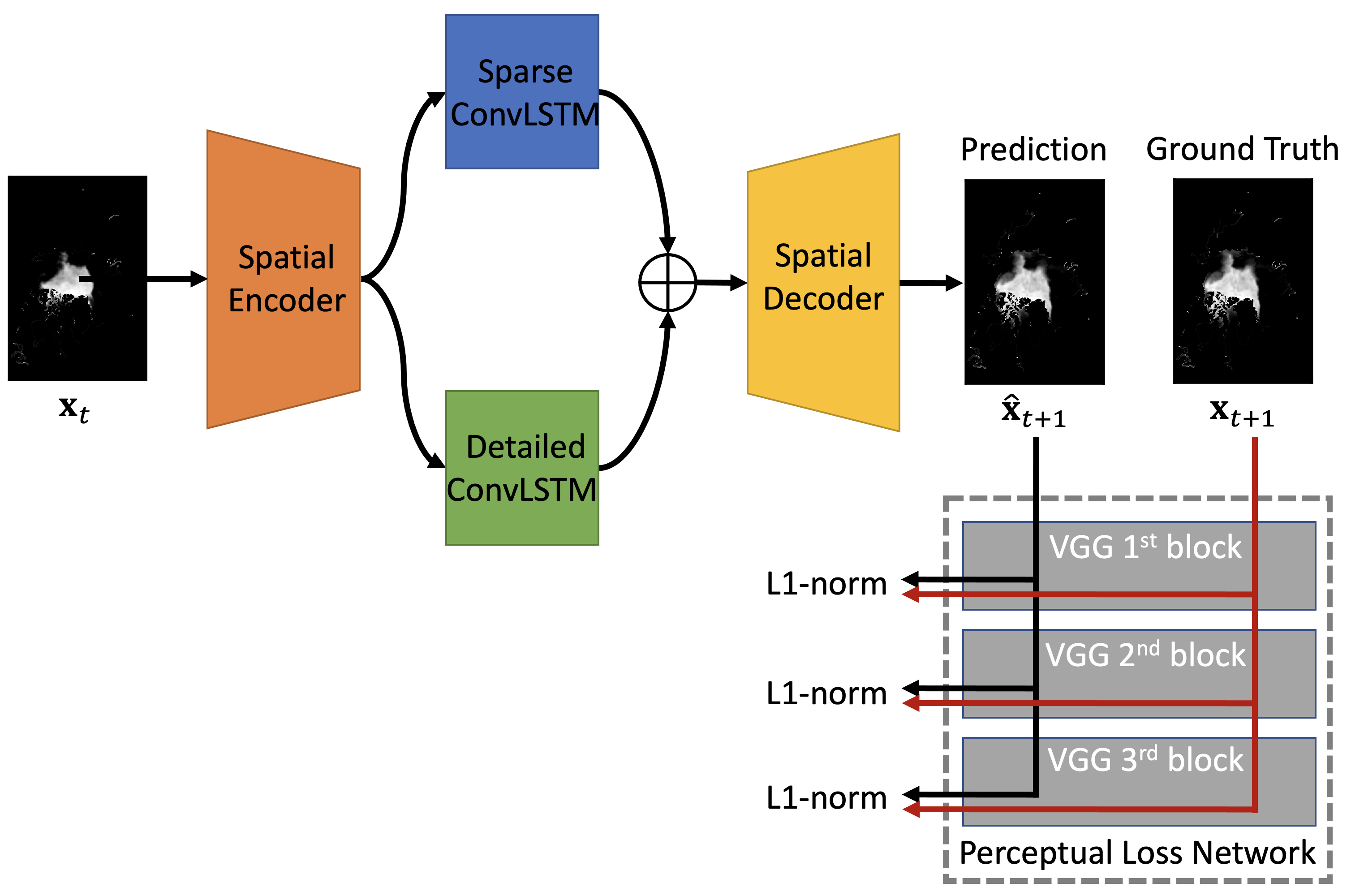
3.1.2. Proposed Model: Two-Stream ConvLSTM

Conventional ConvLSTM captures the spatiotemporal characteristics in prediction problems. As addressed above, although ConvLSTM learns various feature maps from the CNN part, the type of spatiotemporal characteristics to be learned depends on the kernel size and the network depth. Sea ice changes and motions show different characteristics within the Arctic oceans. Although there are no significant changes in ice concentrations or motions in multi-year ice zones and winter seasons, the changes in the first-year ice zones or summer seasons are dynamic. In particular, owing to recent global warming, these changes have accelerated and become difficult to predict. In addition, a combination of more than two networks with different configurations, which learn different data characteristics, showed better outcomes than a single type model [38,39,40,41].

Therefore, this study proposes a sequence-to-sequence Two-Stream ConvLSTM (TS-ConvLSTM) architecture by combining two ConvLSTM with different modalities to learn both fast/slow and sparse/detailed characteristics of sea ice dynamics. The proposed model is comprised of four components: a CNN-based encoder, ConvLSTM-based sparse and detailed learners, and a CNN-based decoder.

Figure 2a shows a detailed block of the proposed architecture. First, a compiled input image (448 × 304 × n; n depends on the number of input variables used) at a given time t ($x_t$) in the sequence data passed through the encoder, which consists of six convolutional layers with 8, 16, 32, 32, 64, and 64 filters, respectively. It extracted feature maps and reduced image size using a 3 × 3 kernel. The output size of the encoded image was 112 × 76 × 64. Then, the sparse and detailed learners took the encoded information and learned the spatiotemporal features separately. The sparse learner extracted the overall position and patterns of sea ice images using a shallow network with a large kernel (i.e., one layer with 64 hidden states ($h^S$); 7 × 7 kernel). The detailed learner learned residual features such as unknown factors, textures, and details, using a deeper network with a small kernel (i.e., three layers with 128, 128, and 64 hidden states ($h^D$), respectively; 3 × 3 kernel). Hidden states from each learner for the next time stamp t + 1 ($h_{t+1}^S$ and $h_{t+1}^D$) were concatenated and then fed into the decoder to produce a predicted image at t + 1 (${\widehat{x}}_{t+1}$). The decoder consists of six up-convolutional layers (i.e., 64, 32, 32, 16, 8, and n filters, respectively; 3 × 3 kernel) to restore images of the original size. We used skip connections between the encoder and decoder to prevent the loss of encoded features.

Figure 2b shows an overview of the pipeline for sequence-to-sequence predictions based on individual blocks (Figure 2a). All hidden states were used as inputs for the two parallelized learners (i.e., blue and green arrows). In the prediction part, the predicted image from the individual block was reinjected as the next input for the individual block.

3.2. Loss Functions

Because the loss function is a navigator of how the model finds an optimal solution of the DL model, selecting appropriate loss functions is essential to determine the performance of the model. The L1-norm (i.e., mean absolute error) and L2-norm (i.e., mean square error) are the most widely used loss functions. The L1-norm is intuitive, less sensitive to outliers, and produces sparser solutions. The L2-norm has better precision than L1, but it is sensitive to outliers as it strongly penalizes large errors. However, in our sea ice prediction problem, we observed large discrepancies between the number of statistical errors and the visual differences (this is demonstrated in Section 4.2). Accordingly, we investigated two feature-based loss functions: structural similarity (SSIM) loss and CNN-based loss–to overcome this limitation.

SSIM is used as a metric correlated with the perception of the human visual system using a combination of correlation, luminance, and contrast, instead of traditional error summation metrics such as mean square error (MSE) or peak signal-to-noise ratio (PSNR) [42]. From a human visual perspective, because SSIM is normalized, while MSE and PSNR are not, the treatment of SSIM is easier than MSE and PSNR. The SSIM between the two images x and y can be defined as follows:

$$\begin{array}{c}\mathrm{SSIM}\left(x,y\right)=l\left(x,y\right)c\left(x,y\right) s\left(x,y\right)\\ l\left(x,y\right)=\frac{2{\mu }_x{\mu }_y+C_1}{{\mu }_x^2+{\mu }_y^2+C_1}\\ c\left(x,y\right)=\frac{2{\sigma }_x{\sigma }_y+C_2}{{\sigma }_x^2+{\sigma }_y^2+C_2}\\ s\left(x,y\right)=\frac{{\sigma }_{xy}+C_3}{{\sigma }_x{\sigma }_y+C_3}\end{array}$$

(1)

where $l\left(x,y\right)$, $c\left(x,y\right)$, and $s\left(x,y\right)$ are the luminance, contrast, and structural similarity, respectively. $\mu$ and $\sigma$ are the average and standard deviations of the image, respectively. ${\sigma }_{xy}$ is the covariance of x and y. $C_1$, $C_2$, and $C_3$ are small constant values to stabilize the division with a weak denominator.

We propose a new feature-based loss using various feature maps generated by a widely used visual geometry group (VGG) model. VGG is a CNN-based model developed by the University of Oxford, and it won second place in the ImageNet Large Scale Visual Recognition Challenge in 2014 [43]. The image is passed through a stack of convolutional layers, where the 3 × 3-filters (the smallest size to capture the notion of left/right, up/down, center) were used. One pixel of the convolution stride was used. The spatial padding of the convolutional layer input preserved the spatial resolution after convolution. Max pooling is performed over a 2 × 2-pixel window, with a stride of 2 followed by some convolutional layers. VGG is configured by a depth of 16 or 19 weighted layers. Johnson et al. [44] used a VGG network for perceptual losses in real-time style transfer and super-resolution; it outperformed the per-pixel loss function, particularly in reconstructing sharp edges and fine details. In our study, we used 16-layer configurations, referred to as VGG16. The original architecture of VGG16 takes fixed size 224 × 224-RGB images, but we inserted an encoding layer using 1 × 1 convolution filters to take any input channels (i.e., a linear transformation of the input channels) such as 448 × 304 × 6 images of sea ice properties and ERA5 variables, as listed in Table 1. The other structures were the same as those of the original VGG16, as illustrated in Figure 3. VGG16 has five main blocks that end in a max-pooling layer. We collected feature maps for each of the last convolutional layers in each block. However, we used the first three blocks because the output image sizes of the 4th and 5th blocks were too small, and our image datasets were relatively simple compared to widely used RGB image datasets. Therefore, 64, 128, and 256 feature maps from the first three blocks were sufficient to capture diverse spatial characteristics. We used pretrained weights without end-to-end training. For the 448 feature maps from VGG16, we used the L1-norm to calculate the total loss.

3.3. Sensitivity of Input Variables

Although our previous study [13] developed a DL-based SIC prediction model using only historical SIC data, follow-up studies [13,14,15,16] used additional input variables related to the ice-ocean-atmosphere in their DL models. In the most recent study conducted by [16], SIC and SIC_ano acquired one year before showed the most significant contributions to the CNN-based prediction model rather than other variables. Because our prediction model was designed for multiple-step predictions, it is worthwhile to test the sensitivity of the input variables. Feature permutation tests using randomly varying single features are widely used to evaluate the feature importance in machine learning tasks [16,45]. Feature permutation tests can be conducted without model retraining because it uses a fully trained model and varies the values of the single test feature. The importance is then ranked based on the relative difference, which is not intuitive. Therefore, in this study, we developed ten independent prediction models using different input variable selections, as defined in

Table 2. A comparison of the sensitivity of the prediction models with varying combinations of input variables.

	M1	M2	M3	M4	M5	M6	M7	M8	M9	M10
SIC	✓	✓	✓	✓	✓	✓	✓	✓	✓	✓
SICano		✓	✓	✓	✓	✓	✓	✓	✓	✓
SIE			✓	✓	✓	✓
T2m				✓	✓	✓	✓			✓
V10m					✓	✓		✓
U10m						✓			✓	✓

. SIC was used in all the models. In M2–M6, we sequentially added one input variable. Input variables for M7–M10 were defined based on the results of M1–M6 (additional details are presented in Section 4.3).

3.4. Training and Testing of Model

Sequence data for the periods 1979–2017, 2018–2019, and 2020 were used for training, validation, and testing, respectively. Several techniques were applied for training to affect robustness and efficiency.

First, adequate training data are required to produce robust models, but obtaining relevant data is limited. Data augmentation can improve the ability of the model to generalize and apply that to new data [46], particularly to those unobserved environmental phenomena that have occurred in the past. Transformations of existing data, such as flips, translations, or rotations, can expand the training data. While training a model, we applied a combination of left-, right-, up-, and down flips and reversed the time sequence with 50% probability. Therefore, our model increased the chances of spatiotemporal learning of new cases. Second, an encoder–decoder architecture for sequence-to-sequence prediction models reinjects the output from the last time step (t−1) as the input for the model at the current time step (t). This recursive output-as-input process can result in slow convergence and model instability owing to incorrect predictions at the early training stages. To remedy these limitations, we used the teacher forcing strategy for quick and efficient training of the recurrent neural network (RNN) models by using the ground truth from a previous time step as input [47]. However, with teacher forcing, predictions can be biased toward performing well only on the exposed past data owing to their over-exposure to the ground truth during training [48]. To maximize the efficiency and stability of the model, we varied the teacher forcing ratio according to the training epochs. For example, at the beginning of model training, we used teacher forcing with near 100% probability, but we reduced the ratio as training progressed. Accordingly, after 100 training epochs, we trained the model without teacher forcing. Finally, we decayed the learning rate with cosine annealing for efficient learning and avoiding local minima present on the stochastic gradient descent.

The models were trained on eight NVIDIA Tesla V100 (32 GB memory) GPUs until the validation loss converged to its minimum after ~120 epochs. The PyTorch (https://pytorch.org accessed on 1 July 2021) framework was used to implement the models.

3.5. Evaluation Metrics

Various error metrics were used to evaluate the performance of the prediction model. Statistical accuracy for SIC values is important, but for sea ice predictions, determining ice-covered or not ice-covered pixels is also important. Therefore, in addition to the mean absolute error (MAE), root mean square error (RMSE), and SSIM, the harmonic mean of the precision and recall (F1 score) was compared and defined according to Equation (2):

$$\begin{array}{c}\mathrm{F}1 \mathrm{score}=2\times \frac{\mathrm{Precision} \times \mathrm{Recall}}{\mathrm{Precision} + \mathrm{Recall}}\\ \mathrm{Precision}=\frac{\mathrm{True} \mathrm{positives}}{\mathrm{True} \mathrm{positives} + \mathrm{False} \mathrm{positives}}\\ \mathrm{Recall}=\frac{\mathrm{True} \mathrm{positives}}{\mathrm{True} \mathrm{positives} + \mathrm{False} \mathrm{negatives}}\end{array}$$

(2)

Because open water (SIC < 5%) and highly concentrated (>50%) pixels are relatively easy to predict, we evaluated pixels ranging from 5% to 50% to calculate F1 scores. To determine the existence of sea ice for these pixels, a threshold of 15% was used to combine both statistical error and visual agreement between the observed and predicted images, and to maximize the difference in errors, MAE/F1 was applied.

4. Experimental Results

Experiments were conducted to compare and demonstrate the performance of the prediction models, loss functions, and input variables for the six-month Arctic sea ice predictions.

4.1. Comparison of Prediction Models

Table 3. Statistical comparisons according to model architectures.

		MAE	RMSE	SSIM	F1	MAE/F1
Prediction models	Persistence	3.0439	9.5741	0.9528	0.7526	4.0447
	LSTM	2.9917	9.1791	0.9501	0.7438	4.0112
	ConvLSTM	2.6904	8.0059	0.9603	0.7687	3.5209
	TS-ConvLSTM	2.3130	7.0274	0.9617	0.7772	3.0157

summarizes the average accuracies for the six-month predictions of the models described in Section 3.1. Figure 4 illustrates the performance of the statistical model according to the lead-time. In this experiment, we used SIC data as inputs and the L1-norm as a loss function for all models to consistently compare the statistical performance based on the model types. As shown in Table 3 and Figure 4, there were no significant statistical benefits in the LSTM model compared to the persistence model. However, ConvLSTM-based models, including the proposed TS-ConvLSTM, significantly outperformed the persistence and LSTM models in all error metrics. As shown in Figure 4, the errors of the DL models were the smallest at t+1, but the errors rapidly increased as the lead-time increased. The proposed TS-ConvLSTM model had the smallest prediction error at t+1, and the variations according to the lead-time were also the smallest among all prediction models. LSTM generally predicted well for the first few steps compared to the persistence model, but errors were higher than the persistence model for later steps. The ConvLSTM-based models consistently outperformed the persistence and LSTM models for future steps. Remarkably, the proposed TS-ConvLSTM had the smallest mean and standard deviation of errors for six-month predictions among all models. Therefore, we used the proposed TS-ConvLSTM model.

4.2. Loss Comparison

This experiment used the proposed TS-ConvLSTM model and SIC data as inputs to compare various loss functions. The statistical mean errors between the observed and predicted images are calculated in

Table 4. Statistical comparisons according to loss functions.

		MAE	RMSE	SSIM	F1	MAE/F1
Loss function	L1-norm	2.3130	7.0274	0.9617	0.7772	3.0157
	L2-norm	2.5347	7.1096	0.9528	0.7482	3.4337
	SSIM	2.3764	7.2373	0.9648	0.7852	3.0836
	VGG	2.2480	6.8250	0.9641	0.7864	2.8922

according to the loss functions.

Error minimization achieved by model training depends on the type of loss function used. For example, as shown in Table 4, a relatively small MAE value was achieved because the L1-norm was based on the absolute error (Note: VGG uses the L1-norm to calculate the differences between feature maps). Similarly, compared to the other error metrics, SSIM loss had a relatively good SSIM value. However, the high F1 scores of the SSIM and VGG loss functions indicated that these perceptual loss functions might improve the predictability of sea ice boundaries or low SIC zones compared to the mathematical loss functions. The overall statistical differences between the loss functions are trivial compared to the differences between the model types, but we observed significant visual differences in the resulting images. Figure 5 illustrates examples of prediction results according to different loss functions. Visual inspections show that even though the differences in the values of MAE and RMSE for each loss function were not significant, the sea ice boundaries in the resulting images were significantly different. Large sea ice distributions connecting to the coastlines of Russia in the East Siberian Sea were present in the observed image (see yellow dashed rectangles). However, as seen in the predicted images using the L1-norm and L2-norm loss functions, these spatially characterized sea ice patches did not exist. The SSIM loss predicted these unique sea ice distributions better than the L1- and L2-norms. The proposed VGG loss function successfully predicted the spatial characteristics of the East Siberian Sea. However, these characterized sea ice patches moved toward the Laptev Sea as the lead-time increased. Based on quantitative and qualitative analyses, the VGG loss predicted the spatial distribution of sea ice with better statistical accuracy compared to other loss functions.

One possible explanation is that the proposed VGG loss is close to human vision. While the L1- and L2-norms are simply calculated using pixel-by-pixel statistics of the single resulting image, and the SSIM can be compared only to the three structural features, the VGG loss generated 448 feature maps. Figure 6 illustrates the sample feature maps from the last convolutional layers of the first three blocks. As shown, the feature maps provide information such as edges and shapes. The convolutional filter detected the bright areas and thereby achieved its purpose. Some feature maps retained most of the sea ice information in the image, acted as edge detectors, or captured the overall shapes of sea ice. In general, while the convolution filters in the first layers detect simple edges or shapes, the feature maps in the deeper network capture an abstract, complex, and sparse representation of the original image. Accordingly, VGG may capture perceptual characteristics that are similar to those of human vision. Although statistical accuracy is a fundamental metric for evaluating the performance of the prediction model, we believe that visual agreements may prove beneficial for appropriate applications.

4.3. Input Variable Comparison

Based on previous experiments, we chose the proposed TS-ConvLSTM with a VGG loss function.

Table 5. Statistical comparisons according to the combinations of input variables.

Avg.	M1	M2	M3	M4	M5	M6	M7	M8	M9	M10
MAE	2.2480	2.2484	2.4248	2.3048	2.3241	2.2936	2.2768	2.2721	2.4822	2.3946
RMSE	6.8250	6.6659	7.1526	6.7504	6.7499	6.6584	6.8210	7.3290	6.8440	7.0379
SSIM	0.9641	0.9611	0.9583	0.9617	0.9609	0.9607	0.9628	0.9375	0.9460	0.9581
F1	0.7864	0.7833	0.7737	0.7885	0.7808	0.7882	0.7848	0.7734	0.7812	0.7724
MAE/F1	2.8922	2.8764	3.1992	2.9667	3.0413	2.9456	2.9490	3.5472	3.2053	3.1428
Std. Dev.	M1	M2	M3	M4	M5	M6	M7	M8	M9	M10
MAE	0.5601	0.4515	0.5980	0.5186	0.4694	0.5010	0.5427	0.5178	0.4682	0.5248
RMSE	1.4970	1.1525	1.6554	1.3358	1.2441	1.1900	1.4999	1.3183	1.1999	1.4581
SSIM	0.0139	0.0103	0.0148	0.0141	0.0141	0.0130	0.0141	0.0118	0.0125	0.0136
F1	0.0434	0.0342	0.0452	0.0400	0.0466	0.0425	0.0404	0.0346	0.0369	0.0384
MAE/F1	0.7627	0.5899	0.8787	0.6831	0.6551	0.6515	0.7265	0.7040	0.6352	0.7118

summarizes the statistical accuracies of the prediction models based on the combinations of input variables. As mentioned in Section 3.3, we sequentially added each feature to M1–M6. As seen in the results of M3, when we added SIE, all types of model accuracies deteriorated notably. Therefore, we excluded the SIE variable in M7– M9 and tested the T_2m, V_10m, and U_10m variables. As a result of M8, when V_10m was added, the errors increased again. Accordingly, M10 excluded V_10m and finally used SIC, SIC_ano, T_2m, and U_10m as input variables. Based on the overall accuracies of the considered error metrics in Table 5, M1, M2, and M4–M7 showed good predictability, but the differences between these models were not significant. Notably, there were no significant improvements when using the SIE and ERA5 variables. We also compared the standard deviations of the errors for each model. The standard deviations tended to decrease with the increase in input variables used. However, M2 had the smallest standard deviation of errors compared to the other models, indicating that M2 showed stable predictability. The statistical accuracy of the prediction model is the most fundamental factor, but the efficiency of data collection and the stability of predictability is also crucial in operational systems. Based on the experimental results, SIC and SIC_ano were the most valuable variables for developing the most accurate, efficient, and stable prediction model.

4.4. Experimental Results for 2020

Based on the previous three experiments, that is, comparisons of the models, losses, and input variables, the best architecture for the six-month predictions of the Arctic sea ice was the proposed TS-ConvLSTM model with VGG loss using the past 12-month SIC and SIC_ano data as inputs. The proposed TS-ConvLSTM significantly reduced the prediction errors compared to the other baseline models (see Section 4.1). The feature-based loss function effectively captured sea ice distributions while maintaining statistical accuracy (see Section 4.2). However, incorporating additional input variables, such as ocean and atmospheric parameters, did not result in an improvement in predictability as expected (see Section 4.3).

Figure 7 shows the statistical comparisons of the proposed prediction model according to lead-time (Figure 7a) and month (Figure 7b), and all statistics are listed in

Table 6. Statistics of prediction errors according to lead-time and month.

MAE	Jan	Feb	Mar	Apr	May	Jun	Jul	Aug	Sep	Oct	Nov	Dec
t+1	1.5449	1.6073	1.9119	2.0731	2.1925	2.3110	1.9762	1.4274	1.3749	1.6131	2.1307	1.5121
t+2	1.8651	1.9391	2.2336	2.6025	2.6588	3.0276	2.2576	2.0488	1.5990	2.2147	2.3257	2.0685
t+3	1.7661	1.9172	2.3787	2.6064	2.6328	3.1759	2.6029	2.1151	1.7610	1.9262	2.5185	2.1391
t+4	1.7501	1.9257	2.2756	2.6432	2.8337	3.2640	2.6258	2.2361	1.7602	2.1307	2.5406	2.1382
t+5	1.7408	1.9589	2.3791	2.7415	2.9673	3.0936	2.5449	2.2148	1.8593	2.5055	2.7582	2.1568
t+6	1.8103	1.9429	2.3729	2.7009	2.9537	3.1456	2.4645	2.1787	1.8640	2.3840	2.8797	2.0871
RMSE	Jan	Feb	Mar	Apr	May	Jun	Jul	Aug	Sep	Oct	Nov	Dec
t+1	4.5148	4.4901	5.4807	5.6759	5.9136	6.3384	6.2614	4.9205	5.4771	5.1247	5.7645	4.1212
t+2	5.4400	5.5926	6.5878	7.8104	7.5234	8.1855	6.6227	6.8165	5.5151	7.1589	6.2950	5.6306
t+3	5.1743	5.3749	7.0786	7.6140	7.3080	8.6651	7.5839	7.1062	7.0182	6.0830	6.7504	5.9125
t+4	5.0823	5.5483	6.6607	7.8540	7.9402	8.8780	7.5768	7.4978	7.2786	6.6463	6.7005	5.8293
t+5	5.1137	5.5092	7.0488	7.9020	8.2512	8.6228	7.4925	7.3205	7.6022	7.5872	7.3328	5.9219
t+6	5.2537	5.5314	7.0453	7.7836	8.2356	8.6377	7.1290	7.1325	7.6024	7.9469	7.8677	5.6516
SSIM	Jan	Feb	Mar	Apr	May	Jun	Jul	Aug	Sep	Oct	Nov	Dec
t+1	0.9789	0.9811	0.9738	0.9666	0.9650	0.9653	0.9635	0.9757	0.9763	0.9648	0.9585	0.9766
t+2	0.9720	0.9737	0.9681	0.9567	0.9527	0.9490	0.9500	0.9602	0.9637	0.9559	0.9561	0.9693
t+3	0.9735	0.9735	0.9636	0.9546	0.9549	0.9490	0.9387	0.9615	0.9675	0.9578	0.9534	0.9689
t+4	0.9735	0.9734	0.9658	0.9512	0.9554	0.9500	0.9384	0.9586	0.9662	0.9553	0.9546	0.9683
t+5	0.9745	0.9731	0.9639	0.9491	0.9527	0.9518	0.9466	0.9585	0.9648	0.9505	0.9503	0.9675
t+6	0.9723	0.9729	0.9651	0.9502	0.9513	0.9499	0.9472	0.9599	0.9654	0.9525	0.9403	0.9673
F1	Jan	Feb	Mar	Apr	May	Jun	Jul	Aug	Sep	Oct	Nov	Dec
t+1	0.8161	0.8231	0.8188	0.8143	0.8156	0.8088	0.7811	0.7978	0.7642	0.7610	0.7812	0.8150
t+2	0.8128	0.8170	0.8147	0.7959	0.8045	0.7902	0.7514	0.7475	0.7459	0.7440	0.7813	0.8113
t+3	0.8133	0.8179	0.8114	0.7992	0.8030	0.7869	0.7407	0.7502	0.7253	0.7487	0.7770	0.8120
t+4	0.8130	0.8182	0.8118	0.7985	0.8018	0.7841	0.7393	0.7254	0.7202	0.7399	0.7789	0.8125
t+5	0.8144	0.8176	0.8142	0.7969	0.7988	0.7879	0.7401	0.7410	0.7156	0.6905	0.7767	0.8129
t+6	0.8129	0.8180	0.8156	0.7984	0.7987	0.7878	0.7451	0.7484	0.7171	0.7177	0.7755	0.8129
MAE/F1	Jan	Feb	Mar	Apr	May	Jun	Jul	Aug	Sep	Oct	Nov	Dec
t+1	1.8929	1.9527	2.3349	2.5458	2.6883	2.8572	2.5302	1.7891	1.7991	2.1198	2.7274	1.8554
t+2	2.2946	2.3735	2.7415	3.2699	3.3050	3.8314	3.0046	2.7407	2.1438	2.9765	2.9766	2.5497
t+3	2.1715	2.3439	2.9314	3.2614	3.2786	4.0360	3.5141	2.8193	2.4279	2.5728	3.2413	2.6344
t+4	2.1527	2.3537	2.8032	3.3103	3.5343	4.1629	3.5518	3.0824	2.4442	2.8796	3.2619	2.6317
t+5	2.1377	2.3959	2.9221	3.4401	3.7148	3.9264	3.4387	2.9887	2.5983	3.6285	3.5509	2.6533
t+6	2.2270	2.3751	2.9093	3.3828	3.6979	3.9929	3.3077	2.9112	2.5995	3.3218	3.7131	2.5673

. Figure 8 illustrates the prediction results for 2020. Overall, as seen in Figure 7a, predictability became weak as the lead-time increased (i.e., MAE, RMSE, and MAE/F1 increased, whereas SSIM and F1 scores decreased). Variations at t+1 were the smallest, but they increased for the long-term predictions owing to the characteristics of the RNN. Notably, the proposed model captured the recent trends and characteristics of sea ice distributions well using the recently updated sea ice data. For example, as shown in Figure 8, for the September predictions, unique sea ice distributions in the Beaufort Sea were clearly identified in t+1 and t+2 images. However, these characteristics were merely present or not observed in the prediction of the images at t+3 to t+6. The extremes of the SIC (open water and high-SIC regions) showed relatively good agreements with the observations regardless of the lead-time as seen in Figure 8, but the differences and errors were mainly observed in the marginal ice zones (20% < SIC < 80%).

As seen in Figure 7b, in freezing months (December–April), statistical accuracies such as MAE, RMSE, and MAE/F1 were relatively low compared to those in summer, although there were more sea ice pixels in winter. However, for the months between the melt and freezing onset, the predictability was weak because of increased sea ice dynamics and the recently accelerating global warming effect. Overall, owing to the large number of open-water pixels and the minimum sea ice, the average MAE, RMSE, and MAE/F1 for September were relatively good compared to the other summer months. However, since F1 scores were calculated for SIC pixels ranging from 5%–50%, which are challenging to predict the range for, September’s F1 scores were lower than that of the others.

5. Discussion

DL-based prediction models using historical remote sensing data have gained attention in many environmental applications in recent years. Because DL-based prediction models show reasonable predictability, they are now used as an alternative to conventional statistical and numerical models. In this study, three research questions were raised: (1) Which types of DL models are appropriate for predicting Arctic sea ice? (2) Is a loss function critical for learning sea ice patterns? (3) Which input variables should be used for an efficient and stable model? To address these questions, we conducted experiments to compare DL model architectures and loss functions and to test input variables using individually trained models instead of relative feature significant tests.

The selection of the proper model is critical for developing an accurate prediction model. Owing to the high relationship between the current and previous year SICs, the statistical accuracy of the persistence model was not poor. Recurrent models worked well in the first few steps but degraded predictability when going further into the future. The overall accuracy of the pixel-wise LSTM model was better than that of the persistence model; however, for longer lead times, it showed more significant errors (see Figure 4). ConvLSTM-based models, including the proposed TS-ConvLSTM, consistently outperformed the persistence and LSTM models for up to six months. However, errors increased as the lead-time increased owing to the nature of the multi-step predictions. The use of different modalities in the proposed model architecture further improved prediction accuracy.

For the second question, the loss function is critical for determining statistical accuracy as well as the overall sea ice distributions or shapes. As compared and discussed in [49], the selection of the proper loss function led to successful estimations. Image quality assessment metrics such as SSIM prevented blurry effects in the predicted images, unlike the conventional global-evaluating loss functions such as the L1-norm or L2-norm using less computational resources. In our study, feature maps from pretrained CNN networks further improved the learning of local patterns. However, the blurry effects for long-term predictions when using the L1-norm or L2-norm discussed in [49] were not observed as lead-time increased because the time periods for our monthly sea ice prediction problem are based on six future steps. While we used the pretrained networks, the proposed VGG loss function was not a computationally cheap solution compared to the SSIM because of the large number of feature maps that needed to be evaluated. Unlike the statistical differences between the model architectures, those between the loss functions were not significant. However, incorporating feature maps from the CNN architecture into the proposed perceptual loss function has the merits of learning and predicting better local distributions and patterns of Arctic sea ice.

Finally, we expected that the atmosphere-related variables were important to improve predictability, but they were not as effective as expected. Due to the characteristics of DL architectures, which learn complicated and nonlinear connections in hidden layers, the importance of input variables seems to be trivial or depends on the model types and the target months. For example, as discussed in [16], forecast albedo was an important variable for September predictions using the random forest model, but this variable was not significant in other cases such as annual predictions or September predictions using the CNN model. We used ERA5 variables acquired during the same period as that of the sea ice data. There might be some time lag between the atmospheric and sea ice variables. For example, the minimum SIE was observed in September, whereas the air temperature in the Arctic was high in July [50]. In this study, the time lags between the input variables were not considered, and this could possibly be the reason for the inability in developing a better prediction model by adding atmospheric variables. Furthermore, the 10 m wind speed is essential for sea ice modeling because it determines the surface wind stress, which is the primary force responsible for ice motion. Wind speed and direction in the Arctic are closely controlled by cyclone activity. Serreze et al. [51] noted the impact of summer cyclone activity on sea ice loss. Cyclones can spread out ice to cover a larger area and form spaces between ice floes. This accelerates ice loss because the dark ocean water absorbs more solar energy and increases melting. Contrastingly, high cyclone activity in May, June, and July leads to a higher-than-average September SIE. Some storms can bolster the ice [52,53], and they can occasionally strengthen the ice pack by bringing in cold air. Snow from the storm falls on the ice, which can help to reinforce ice by increasing the sunlight reflection and further help to keep temperatures down. Arctic winds can have both positive and negative effects on the growth and retreat of the Arctic sea ice. These conflicting effects may attenuate the outcome.

Although the proposed approaches in this study were successfully incorporated into the six-month Arctic sea ice prediction compared to the pixel-wise LSTM or the vanilla ConvLSTM model, challenges remain. First, we demonstrated that atmospheric parameters were not significant, and therefore, a further investigation of the time lags between input variables caused by environmental phenomena must be explored. Utilizing sea ice motion and thickness, first ice-free date, different climatological scenarios, and CO₂ concentration scenarios [54] may further improve the prediction accuracy and robustness. Second, the ConvLSTM was widely used in the prediction of the video frames that contain continuous image information, but the monthly sea ice data used in this study were temporally sparse. Capturing these dynamic and subtle sea ice changes using sparse monthly data may be limited because there are significant changes in sea ice distributions and patterns during summer. On the other hand, daily data contain large inter-day variability, and there are no significant daily changes, or the changes may be within daily uncertainties in satellite records. Therefore, the selection of optimal prediction frequencies (3-day or weekly data) and frequent predictions are beneficial for applications such as marine navigation and understanding the subtle differences in sea ice changes. Finally, although the proposed VGG loss function mimics human vision and improves both quantitative and qualitative accuracies, the pretrained VGG network may not be optimal for sea ice data. Many feature maps may contain redundant information. Therefore, retraining and optimizing the VGG network or the more efficient CNN-based networks such as ResNet [55] and EfficientNet [56] using sea ice data are worth investigating.

6. Conclusions

The present study proposed DL-based Arctic sea ice prediction models, including a new model architecture and a perceptual-loss function. We also tested the impact of the input variables using several combinations. As a result, owing to the seasonal cycle of Arctic sea ice, there were high correlations between the sea ice observed in the same month. The LSTM model did not outperform the persistence model for multi-step-ahead predictions. However, a combination of CNN and LSTM models would benefit from learning both spatial and temporal characteristics. The proposed TS-ConvLSTM captured different spatial characteristics using different network modalities. We also demonstrated that the selection of a proper loss function was critical for capturing sea ice distributions and patterns, although statistical differences between the loss functions were not significant. Additional input variables were less critical than expected, but the addition of input variables slightly reduced the uncertainties in the predictions. Overall, the proposed TS-ConvLSTM model using the perceptual VGG loss function and input variables of SIC and SIC_ano produced the most accurate and efficient monthly predictions of Arctic sea ice.

References

1. Thackeray, C.W.; Hall, A. An emergent constraint on future Arctic sea-ice albedo feedback. Nat. Clim. Chang. 2019, 9, 972–978. [Google Scholar] [CrossRef]
2. Najafi, M.R.; Zwiers, F.W.; Gillett, N.P. Attribution of Arctic temperature change to greenhouse-gas and aerosol influences. Nat. Clim. Chang. 2015, 5, 246–249. [Google Scholar] [CrossRef]
3. Stroeve, J.; Holland, M.M.; Meier, W.; Scambos, T.; Serreze, M. Arctic sea ice decline: Faster than forecast. Geophys. Res. Lett. 2007, 34. [Google Scholar] [CrossRef]
4. Vihma, T. Effects of Arctic Sea Ice Decline on Weather and Climate: A Review. Surv. Geophys. 2014, 35, 1175–1214. [Google Scholar] [CrossRef] [Green Version]
5. Meier, W.; Bhatt, U.S.; Walsh, J.; Thoman, R.; Bieniek, P.; Bitz, C.M.; Blanchard-Wrigglesworth, E.; Eicken, H.; Hamilton, L.C.; Hardman, M.; et al. 2020 Sea Ice Outlook Post-Season Report; Sea Ice Prediction Network: Fairbanks, AK, USA, 2021. [Google Scholar]
6. Screen, J.A.; Simmonds, I. The central role of diminishing sea ice in recent Arctic temperature amplification. Nat. Cell Biol. 2010, 464, 1334–1337. [Google Scholar] [CrossRef] [Green Version]
7. Pithan, F.; Mauritsen, T. Arctic amplification dominated by temperature feedbacks in contemporary climate models. Nat. Geosci. 2014, 7, 181–184. [Google Scholar] [CrossRef]
8. Mioduszewski, J.R.; Vavrus, S.; Wang, M.; Holland, M.; Landrum, L. Past and future interannual variability in Arctic sea ice in coupled climate models. Cryosphere 2019, 13, 113–124. [Google Scholar] [CrossRef] [Green Version]
9. Guemas, V.; Blanchard-Wrigglesworth, E.; Chevallier, M.; Day, J.; Déqué, M.; Doblas-Reyes, F.; Fučkar, N.S.; Germe, A.; Hawkins, E.; Keeley, S.; et al. A review on Arctic sea-ice predictability and prediction on seasonal to decadal time-scales. Q. J. R. Meteorol. Soc. 2016, 142, 546–561. [Google Scholar] [CrossRef]
10. Stroeve, J.; Hamilton, L.C.; Bitz, C.M.; Blanchard-Wrigglesworth, E. Predicting September sea ice: Ensemble skill of the SEARCH Sea Ice Outlook 2008–2013. Geophys. Res. Lett. 2014, 41, 2411–2418. [Google Scholar] [CrossRef] [Green Version]
11. Wang, W.; Chen, M.; Kumar, A. Seasonal Prediction of Arctic Sea Ice Extent from a Coupled Dynamical Forecast System. Mon. Weather. Rev. 2013, 141, 1375–1394. [Google Scholar] [CrossRef]
12. Sigmond, M.; Fyfe, J.C.; Flato, G.M.; Kharin, V.V.; Merryfield, W.J. Seasonal forecast skill of Arctic sea ice area in a dynamical forecast system. Geophys. Res. Lett. 2013, 40, 529–534. [Google Scholar] [CrossRef]
13. Chi, J.; Kim, H.-C. Prediction of Arctic Sea Ice Concentration Using a Fully Data Driven Deep Neural Network. Remote Sens. 2017, 9, 1305. [Google Scholar] [CrossRef] [Green Version]
14. Kim, J.; Kim, K.; Cho, J.; Kang, Y.Q.; Yoon, H.-J.; Lee, Y.-W. Satellite-Based Prediction of Arctic Sea Ice Concentration Using a Deep Neural Network with Multi-Model Ensemble. Remote Sens. 2018, 11, 19. [Google Scholar] [CrossRef] [Green Version]
15. Choi, M.; De Silva, L.W.A.; Yamaguchi, H. Artificial Neural Network for the Short-Term Prediction of Arctic Sea Ice Concentration. Remote Sens. 2019, 11, 1071. [Google Scholar] [CrossRef] [Green Version]
16. Kim, Y.J.; Kim, H.-C.; Han, D.; Lee, S.; Im, J. Prediction of monthly Arctic sea ice concentrations using satellite and reanalysis data based on convolutional neural networks. Cryosphere 2020, 14, 1083–1104. [Google Scholar] [CrossRef] [Green Version]
17. Liu, Q.; Zhang, R.; Wang, Y.; Yan, H.; Hong, M. Daily Prediction of the Arctic Sea Ice Concentration Using Reanalysis Data Based on a Convolutional LSTM Network. J. Mar. Sci. Eng. 2021, 9, 330. [Google Scholar] [CrossRef]
18. Cho, K.; Naoki, K. Advantages of AMSR2 for Monitoring Sea Ice from Space; Citeseer: University Park, PA, USA, 2015; pp. 19–23. [Google Scholar]
19. Ivanova, N.; Johannessen, O.M.; Pedersen, L.T.; Tonboe, R.T. Retrieval of Arctic Sea Ice Parameters by Satellite Passive Microwave Sensors: A Comparison of Eleven Sea Ice Concentration Algorithms. IEEE Trans. Geosci. Remote Sens. 2014, 52, 7233–7246. [Google Scholar] [CrossRef]
20. Cavalieri, D.; Parkinson, C.; Gloersen, P.; Zwally, H.J. Sea Ice Concentrations from Nimbus-7 SMMR and DMSP SSM/I-SSMIS Passive Microwave Data; Version 1; NASA Goddard Earth Sciences Data and Information Services Center: Greenbelt, MD, USA, 2020; p. 25.
21. Spreen, G.; Kaleschke, L.; Heygster, G. Sea ice remote sensing using AMSR-E 89-GHz channels. J. Geophys. Res. Space Phys. 2008, 113, 113. [Google Scholar] [CrossRef] [Green Version]
22. Comiso, J.C. SSM/I Sea Ice Concentrations Using the Bootstrap Algorithm; National Aeronautics and Space Administration, Goddard Space Flight Center: Greenbelt, MD, USA, 1995; Volume 1380.
23. Vinnikov, K.Y.; Robock, A.; Stouffer, R.J.; Walsh, J.E.; Parkinson, C.L.; Cavalieri, D.J.; Mitchell, J.F.B.; Garrett, D.; Zakharov, V.F. Global Warming and Northern Hemisphere Sea Ice Extent. Science 1999, 286, 1934–1937. [Google Scholar] [CrossRef] [PubMed]
24. Hersbach, H.; Bell, B.; Berrisford, P.; Hirahara, S.; Horanyi, A.; Muñoz-Sabater, J.; Nicolas, J.; Peubey, C.; Radu, R.; Schepers, D.; et al. The ERA5 global reanalysis. Q. J. R. Meteorol. Soc. 2020, 146, 1999–2049. [Google Scholar] [CrossRef]
25. Hersbach, H.; Bell, B.; Berrisford, P.; Biavati, G.; Horányi, A.; Sabater, J.M.; Nicolas, J.; Peubey, C.; Radu, R.; Rozum, I.; et al. ERA5 Hourly Data on Single Levels from 1979 to Present. Available online: https://cds.climate.copernicus.eu/cdsapp#!/dataset/reanalysis-era5-single-levels?tab=overview (accessed on 2 June 2021). [CrossRef]
26. Lindsay, R.; Wensnahan, M.; Schweiger, A.; Zhang, J. Evaluation of Seven Different Atmospheric Reanalysis Products in the Arctic. J. Clim. 2014, 27, 2588–2606. [Google Scholar] [CrossRef] [Green Version]
27. Graham, R.M.; Hudson, S.R.; Maturilli, M. Improved Performance of ERA5 in Arctic Gateway Relative to Four Global Atmospheric Reanalyses. Geophys. Res. Lett. 2019, 46, 6138–6147. [Google Scholar] [CrossRef] [Green Version]
28. Dong, X.; Wang, Y.; Hou, S.; Ding, M.; Yin, B.; Zhang, Y. Robustness of the Recent Global Atmospheric Reanalyses for Antarctic Near-Surface Wind Speed Climatology. J. Clim. 2020, 33, 4027–4043. [Google Scholar] [CrossRef] [Green Version]
29. Greff, K.; Srivastava, R.K.; Koutnik, J.; Steunebrink, B.R.; Schmidhuber, J. LSTM: A Search Space Odyssey. IEEE Trans. Neural Netw. Learn. Syst. 2017, 28, 2222–2232. [Google Scholar] [CrossRef] [PubMed] [Green Version]
30. Gers, F.A.; Schmidhuber, J.; Cummins, F. Learning to Forget: Continual Prediction with LSTM. Neural Comput. 2000, 12, 2451–2471. [Google Scholar] [CrossRef] [PubMed]
31. Srivastava, S.; Lessmann, S. A comparative study of LSTM neural networks in forecasting day-ahead global horizontal irradiance with satellite data. Sol. Energy 2018, 162, 232–247. [Google Scholar] [CrossRef]
32. Rhif, M.; Ben Abbes, A.; Martinez, B.; Farah, I.R. A deep learning approach for forecasting non-stationary big remote sensing time series. Arab. J. Geosci. 2020, 13, 1–11. [Google Scholar] [CrossRef]
33. Shi, X.; Chen, Z.; Wang, H.; Yeung, D.-Y.; Wong, W.; Woo, W. Convolutional LSTM Network: A Machine Learning Approach for Precipitation Nowcasting. arXiv 2015, arXiv:1506.04214. [Google Scholar]
34. Chen, L.; Cao, Y.; Ma, L.; Zhang, J. A Deep Learning-Based Methodology for Precipitation Nowcasting With Radar. Earth Space Sci. 2020, 7, 7. [Google Scholar] [CrossRef] [Green Version]
35. Sun, D.; Wu, J.; Huang, H.; Wang, R.; Liang, F.; Xinhua, H. Prediction of Short-Time Rainfall Based on Deep Learning. Math. Probl. Eng. 2021, 2021, 1–8. [Google Scholar] [CrossRef]
36. Kreuzer, D.; Munz, M.; Schlüter, S. Short-term temperature forecasts using a convolutional neural network—An application to different weather stations in Germany. Mach. Learn. Appl. 2020, 2, 100007. [Google Scholar] [CrossRef]
37. Kim, K.-S.; Lee, J.-B.; Roh, M.-I.; Han, K.-M.; Lee, G.-H. Prediction of Ocean Weather Based on Denoising AutoEncoder and Convolutional LSTM. J. Mar. Sci. Eng. 2020, 8, 805. [Google Scholar] [CrossRef]
38. Donahue, J.; Hendricks, L.A.; Rohrbach, M.; Venugopalan, S.; Guadarrama, S.; Saenko, K.; Darrell, T. Long-Term Recurrent Convolutional Networks for Visual Recognition and Description. IEEE Trans. Pattern Anal. Mach. Intell. 2017, 39, 677–691. [Google Scholar] [CrossRef]
39. Ma, C.-Y.; Chen, M.-H.; Kira, Z.; AlRegib, G. TS-LSTM and temporal-inception: Exploiting spatiotemporal dynamics for activity recognition. Signal Process. Image Commun. 2019, 71, 76–87. [Google Scholar] [CrossRef] [Green Version]
40. Ye, W.; Cheng, J.; Yang, F.; Xu, Y. Two-Stream Convolutional Network for Improving Activity Recognition Using Convolutional Long Short-Term Memory Networks. IEEE Access 2019, 7, 67772–67780. [Google Scholar] [CrossRef]
41. Chi, J.; Kim, H.-C. Retrieval of daily sea ice thickness from AMSR2 passive microwave data using ensemble convolutional neural networks. GIScience Remote Sens. 2021, 1–19. [Google Scholar] [CrossRef]
42. Wang, Z.; Bovik, A.C.; Sheikh, H.R.; Simoncelli, E.P. Image Quality Assessment: From Error Visibility to Structural Similarity. IEEE Trans. Image Process. 2004, 13, 600–612. [Google Scholar] [CrossRef] [Green Version]
43. Simonyan, K.; Zisserman, A. Very deep convolutional networks for large-scale image recognition. arXiv 2014, arXiv:1409.1556. [Google Scholar]
44. Johnson, J.; Alahi, A.; Fei-Fei, L. Perceptual Losses for Real-Time Style Transfer and Super-Resolution. In Computer Vision—ECCV 2016; Springer: Cham, Switzerland, 2016; pp. 694–711. [Google Scholar] [CrossRef] [Green Version]
45. Chi, J.; Kim, H.-C.; Lee, S.; Crawford, M.M. Deep learning based retrieval algorithm for Arctic sea ice concentration from AMSR2 passive microwave and MODIS optical data. Remote Sens. Environ. 2019, 231, 111204. [Google Scholar] [CrossRef]
46. Perez, L.; Wang, J. The Effectiveness of Data Augmentation in Image Classification Using Deep Learning. arXiv 2017, arXiv:1712.04621v1. [Google Scholar]
47. Williams, R.J.; Zipser, D. A Learning Algorithm for Continually Running Fully Recurrent Neural Networks. Neural Comput. 1989, 1, 270–280. [Google Scholar] [CrossRef]
48. He, T.; Zhang, J.; Zhou, Z.; Glass, J. Quantifying Exposure Bias for Open-Ended Language Generation. arXiv 2019, arXiv:1905.10617. [Google Scholar]
49. Tran, Q.-K.; Song, S.-K. Computer Vision in Precipitation Nowcasting: Applying Image Quality Assessment Metrics for Training Deep Neural Networks. Atmosphere 2019, 10, 244. [Google Scholar] [CrossRef] [Green Version]
50. Rigor, I.G.; Colony, R.L.; Martin, S. Variations in Surface Air Temperature Observations in the Arctic, 1979–97. J. Clim. 2000, 13, 896–914. [Google Scholar] [CrossRef]
51. Serreze, M.C.; Maslanik, J.A.; Scambos, T.A.; Fetterer, F.; Stroeve, J.; Knowles, K.; Fowler, C.; Drobot, S.; Barry, R.; Haran, T.M. A record minimum arctic sea ice extent and area in 2002. Geophys. Res. Lett. 2003, 30. [Google Scholar] [CrossRef]
52. Morello, L. Summer storms bolster Arctic ice. Nat. Cell Biol. 2013, 500, 512. [Google Scholar] [CrossRef] [PubMed] [Green Version]
53. Webster, M.A.; Parker, C.; Boisvert, L.; Kwok, R. The role of cyclone activity in snow accumulation on Arctic sea ice. Nat. Commun. 2019, 10, 5285. [Google Scholar] [CrossRef] [PubMed] [Green Version]
54. Chavas, J.-P.; Grainger, C. On the dynamic instability of Arctic sea ice. Npj Clim. Atmospheric Sci. 2019, 2, 23. [Google Scholar] [CrossRef]
55. Kaiming, H.; Xiangyu, Z.; Shaoqing, R.; Jian, S. Deep Learning with Depthwise Separable Convolutions. In Proceedings of the IEEE Conference on Computer Vision and Pattern Recognition (CVPR), Honolulu, HI, USA, 21–26 July 2017; IEEE: New York, NY, USA, 2017; pp. 1251–1258. [Google Scholar]
56. Tan, M.; Le, Q.V. Efficientnet: Rethinking model scaling for convolutional neural networks. arXiv 2019, arXiv:1905.11946. [Google Scholar]
Figure 1. Examples of co-registered (top row) sea ice and (bottom row) atmosphere-related images. All images are mapped onto a polar stereographic 25-km grid.
Remotesensing 13 03413 g001
Figure 2. (a) A detailed block of the proposed TS-ConvLSTM. There are two streams of the backbone networks to learn different characteristics. (b) An overall pipeline of the proposed TS-ConvLSTM for sequence-to-sequence predictions.
Remotesensing 13 03413 g002aRemotesensing 13 03413 g002b
Figure 3. The architecture of VGG16 for the first five blocks. To calculate loss, we used feature maps from the last convolutional layer in the first three blocks.
Remotesensing 13 03413 g003
Figure 4. Statistical accuracy comparisons of the prediction models, including persistence, long- and short-term memory (LSTM), convoluted LSTM (ConvLSTM), and Two-Stream ConvLSTM (TS-ConvLSTM) based on the lead-time. (a) MAE (blue lines) and RMSE (orange lines); (b) SSIM (green lines) and F1 (gray lines).
Remotesensing 13 03413 g004
Figure 5. Visual comparisons of the predicted images based on the loss functions.
Remotesensing 13 03413 g005
Figure 6. Examples of feature maps from the first three VGG blocks.
Remotesensing 13 03413 g006
Figure 7. Box plots for statistical comparisons of the proposed approaches for the unseen test data according to (a) lead-time and (b) month.
Remotesensing 13 03413 g007
Figure 8. The predicted sea ice concentration images for 2020 based on lead-time and month.
Remotesensing 13 03413 g008aRemotesensing 13 03413 g008b