Tree Extraction from Airborne Laser Scanning Data in Urban Areas

Abstract

Tree information in urban areas plays a significant role in many fields of study, such as ecology and environmental management. Airborne LiDAR scanning (ALS) excels at the fast and efficient acquisition of spatial information in urban-scale areas. Tree extraction from ALS data is an essential part of tree structural studies. Current raster-based methods that use canopy height models (CHMs) suffer from the loss of 3D structure information, whereas the existing point-based methods are non-robust in complex environments. Aiming at making full use of the canopy’s 3D structure information that is provided by point cloud data, and ensuring the method’s suitability in complex scenes, this paper proposes a new point-based method for tree extraction that is based on 3D morphological features. Considering the elevation deviations of the ALS data, we propose a neighborhood search method to filter out the ground and flat-roof points. A coarse extraction method, combining planar projection with a point density-filtering algorithm is applied to filter out distracting objects, such as utility poles and cars. After that, a Euclidean cluster extraction (ECE) algorithm is used as an optimization strategy for coarse extraction. In order to verify the robustness and accuracy of the method, airborne LiDAR data from Zhangye, Gansu, China and unmanned aircraft vehicle (UAV) LiDAR data from Xinyang, Henan, China were tested in this study. The experimental results demonstrated that our method was suitable for extracting trees in complex urban scenes with either high or low point densities. The extraction accuracy obtained for the airborne LiDAR data and UAV LiDAR data were 99.4% and 99.2%, respectively. In addition, a further study found that the aberrant vertical structure of the artificially pruned canopy was the main cause of the error. Our method achieved desirable results in different scenes, with only one adjustable parameter, making it an easy-to-use method for urban area studies.

1. Introduction

The term “urban tree” refers to a woody perennial plant growing in cities and the surrounding areas [1]. Urban trees play a crucial role in enhancing environmental quality and are recognized as fundamental to city livability, resilience, and sustainability [2,3]. Specifically, trees improve air quality by absorbing gaseous pollutants through leaf stomata and dissolving water-soluble pollutants onto moist leaf surfaces. Furthermore, tree canopies weaken the urban heat-island effect by reducing air temperature through shading and evapotranspiration. As well as these benefits, trees reduce urban flood risk because stormwater runoff is mitigated by rainwater interception and storage in urban tree canopies [1,4,5]. Finally, urban trees also have important ecological functions in providing habitats for urban wildlife, abating noise, decreasing wind speed, increasing surface runoff and conditioning the urban microclimate [6,7], maintaining urban ecological balance, and protecting biodiversity [8,9,10]. Therefore, accurate, rapid, and effective acquisition of the spatial distribution information about urban trees is critical for supporting numerous strategies of sustainable urban development, urban tree planting, maintenance, and management [11].

Traditionally, urban tree information has been obtained from a field inventory, which is regarded as the primary approach to achieving the most accurate and detailed distribution information of vegetation [12]. However, fieldwork is labor- and time-intensive, making it hard to scale up to larger areas [13,14]. Nowadays, remote-sensing data provide one of the most effective tools for urban tree extraction [15]. Optical sensor-derived data, such as aerial photography and high-resolution satellite imagery, have been used to extract vegetation information based on distinctive spectral and textural features [12]. However, optical remote sensing data is vulnerable to weather conditions and lacks the vertical structure information for mapping urban vegetation [16]. To make up for this shortfall, the introduction of LiDAR technology makes it possible to acquire massive amounts of 3D geospatial information for the trees in urban scenes [17]. In particular, LiDAR is an active remote-sensing technology that measures the properties of reflected laser pulses to determine the range from a distant object [9]. The range to an object is derived by measuring the time delay between the transmission of a laser pulse and the detection of the reflected signal [18]. Owing to its ability to generate 3D data with high spatial resolution and accuracy, tree extraction using LiDAR has entered a new era [19].

LiDAR scanning can be classified into four categories, according to its platform: satellite-based laser scanning (SLS), airborne laser scanning (ALS), mobile laser scanning (MLS), and terrestrial laser scanning (TLS). The SLS data have very sparsely sampled points with tens of meters of data gaps; thus, the datasets are inadequate for urban tree extraction [3]. TLS data have the highest point density and can be used for the retrieval of canopy structure parameters at the individual tree scale [20,21,22]. However, the poor mobility and occlusion problems of TLS make it almost impossible for data collection on an urban scale. Conversely, MLS has been used extensively in recent years for the collection and analysis of tree information in urban areas but with the main focus on street trees [23,24,25]. With regard to the limitations of the vehicle’s sphere of activities, MLS suffers from the inconvenience of detecting trees in traffic-unfriendly areas and struggles to cover the entire urban area. Further to this, in areas around building structures, occlusion leads to a lack of canopy integrity, which can be fatal for tree parameter estimates, such as tree height or canopy width. Owing to the top-down scanning mechanism and the large flight coverage, ALS has the capability of gathering highly accurate and dense point clouds and, thus, is well suited for larger areas and cities [26]. Numerous studies have demonstrated that ALS data can be employed for urban 3D morphology investigations [27], building rooftops extractions, density information acquisitions [28,29,30], urban green volume estimations [31,32], and individual tree detections [33,34,35].

In earlier studies, the detection of tree canopies for ALS data was performed based on the methods developed for optical imagery [36]. By rasterizing the point cloud data into a pixel-sized image, each pixel on the obtained surface can contain certain information from the original point cloud, such as maximum elevation, minimum elevation, number of echoes, and average echo intensity information [37,38]. Based on the rasterized image, abundant algorithms have been proposed to detect trees, which included, but were not limited to, tree-top detection through the slope, local maxima and their corresponding optimizations [39,40], crown segments based on region-growing algorithms [41], as well as watershed analysis [42]. However, the drawbacks of these approaches are obvious. The information regarding vertical structures is inevitably lost when converting the point cloud into a canopy height model [43]. Moreover, the results of the tree detection differ to a great extent by changing the size of the raster, which leads to the issue that the efficiency of these approaches directly relies on the quality of the initial rasterization.

To bypass the abovementioned drawbacks, point-based methods were proposed to process the point cloud data directly. The initial point-based methods were oriented on fairly simple scenes, which contained only trees and the ground. In such cases, ground point filtering has been proposed for the extraction of trees. Over the past two decades, various practical filtering algorithms have been proposed [44,45,46]. By filtering out the ground points, the remaining points were regarded as tree points. As a matter of course, the approaches above suffered from the insufficiency of filtering out other non-ground objects, such as buildings, cars, etc. For complex scenes, a more comprehensive approach is urgently needed since little work has yet been done in this field. Haiquan Yang et al. proposed a tree extraction method [12] based on the 3D fractal dimensions of objects. By quantifying the 3D fractal dimensions of each type of object by means of fractal geometry, tall trees can be distinguished from other objects. Unfortunately, this method also has its shortcomings. The semi-data-driven nature of this approach makes it highly sensitive to the choices of numerous parameters. Although the method can be used in classifying multiple objects, the complexity of the scene it faces is still limited, and the acquirement of training samples also hinders its application in larger and more complex scenes.

To improve the process of tree extraction, we herein propose a new point-based method to extract trees from LiDAR point clouds. Our method aims to (a) extract tree points in complex urban areas with (b) high accuracy, and (c) perform this automatically in an easy-to-use way.

2. Materials and Methods

This study proposes an easy-to-use method for tree extraction, specifically based on the fluctuations of point elevations and the morphological characteristics of tree canopies. The overall workflow is shown in Figure 1. Firstly, the points in flat areas are distinguished from those in undulating areas, based on the integration of the flat distance and elevation difference, which filters out ground and roof points. Then, incorporating morphological characteristics of tree canopies and other interfering objects, a tree point extraction on the basis of point count is established in the undulating areas. Finally, a further tree point refinement step is deployed, using a qualified Euclidean cluster extraction (ECE) algorithm.

2.1. Ground and Flat Roof Point Removal

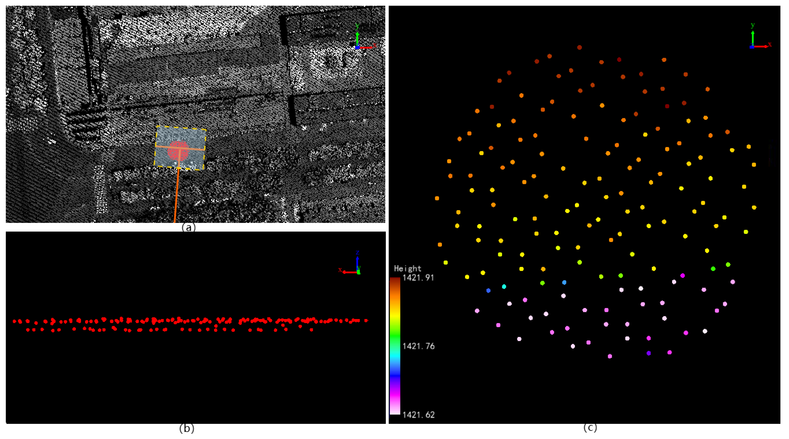
In the process of data collection, measurement deviation is inevitable, due to the complex structure of the flight platform and frequent changes and movement in the environment. At this time, the elevation deviation of the ALS data is on the sub-meter scale [47,48]. When such deviations exist in the elevation of the point cloud data, the uncertainty of flattened areas in the point cloud data needs to be taken into account. In addition, in flat areas such as road surfaces, the existence of potholes on the surface of flat areas due to microtopography (Figure 2) causes the point cloud data to not be absolutely consistent in terms of elevation. Given this, we developed a new algorithm for determining points in flat areas by incorporating the distance between points and the information on height differences. The core idea of this algorithm is that if the height difference between a point and any point within a certain range is greater than a given threshold, then the point is considered to be a non-flat area point, and vice versa. The algorithm can be divided into three steps.

Step 1: pick an arbitrary point $\mathrm{P}$ from the original point cloud data, and collect all points from the original point cloud data whose flat distance $R$ from P is smaller than $R_{\max }$, then name the set of the collected points as $\mathrm{S}$:

$$R=\sqrt{{\left(x_T-x_P\right)}^2+{\left(y_T-y_P\right)}^2},$$

(1)

where $x_T$, $y_T$, $x_P$ and $y_P$ represent the x and y-axis coordinates of points $\mathrm{T}$ and $\mathrm{P}$, respectively. $R_{\max }$ is the largest search radius when collecting the point set S, which is set to the radius of the maximum canopy in the study area (5 m). This ensures that enough points and areas are taken into consideration when determining the flatness around point $\mathrm{P}$. When a point has an R smaller than $R_{\max }$, it belongs to $\mathrm{S}$.

Step 2: calculate the elevation difference $\Delta \mathrm{h}$ between point $\mathrm{P}$ and each point within $\mathrm{S},$ and note the maximum elevation difference $\Delta {\mathrm{h}}_{max}$:

$$\Delta \mathrm{h}=\left|z_t-z_p\right|,$$

(2)

where $z_T$ and $z_P$ represent the z-axis coordinates of points $\mathrm{T}$ and $\mathrm{P}$, respectively.

Repeat Steps 1 and 2 until all points in the original data have been traversed.

Step 3: traverse the original data and eliminate points with a $\Delta {\mathrm{h}}_{max}$ of less than twice the maximum deviation in height.

First, we assume that the road is a flat area, then randomly select ten road sampling areas within a circular window, with $R_{\max }$ as the radius in the original point cloud data (only road points are included in the sampling area, with features such as trees, pedestrians, and vehicles excluded). The difference between the lowest and highest points of each sample is then calculated, the largest value of which is taken as twice the maximum height deviation. In the study area, we found the maximum deviation in height was 0.48 m.

By following the above steps, we can eliminate the vast majority of ground and roof points and, thereby, obtain points in undulating areas. The points remaining are collected as inputs for the coarse extraction of tree points.

2.2. Coarse Extraction of Tree Points

Streetlights and utility poles have a top height of several meters from ground level. Likewise, the edges of the buildings “fall away” from the ground. These segments are easily confused with trees when the researcher is only using the topographic slope determination method. However, these disturbance-creating objects often have a small footprint compared to the canopy, which means that the number of points in these segments is small. Based on the various number of points for heterogeneous objects, we are able to filter out non-tree interference terms.

We can assume that tree crowns tend to have more points than the edges of buildings and poles since they have a larger projection area in the horizonal plane. Based on the variation in the number of points for specific types of objects, our algorithm for filtering out interfering objects is divided into three steps:

Step 1, project the points (the points obtained in Section 2.1) in three dimensions onto the x/y plane;

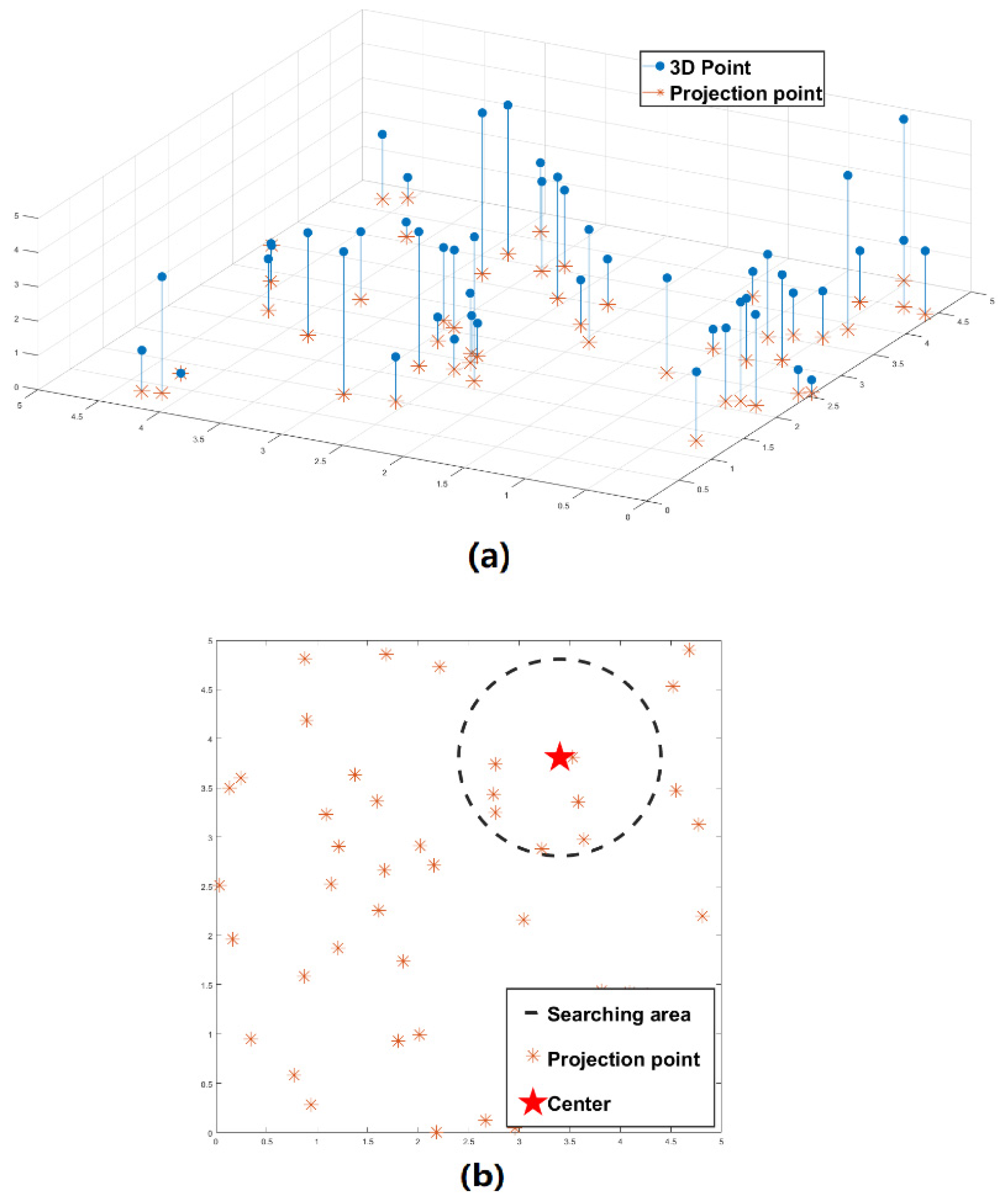
Step 2, pick an arbitrary point, P, among the projected points. Take P as the center of the circle, with a radius of ${\mathrm{R}}_{search}$ as a search area, and count how many points are left in the search area apart from point P, denoted as OPN (other points’ number). Repeat Step 2 until all points have been traversed (Figure 3);

Step 3, since each projected point has a corresponding three dimensions point, collect the three-dimensional points of the projected points with an OPN smaller than an empirical threshold as a point set.

In this study, we set ${\mathrm{R}}_{search}$ the same value of $R_{\max }$ to ensure that enough points are taken into consideration in the step of coarse extraction. The threshold of OPN is proportional to the point density and determined by the specific data.

By following the above steps, we can eliminate the disturbance-creating objects and thereby obtain most tree points. The final collected point set is the input for the fine extraction of tree points.

2.3. Fine Extraction of Tree Points

Through the steps described above, we can eliminate distracting objects. However, as the canopies vary in form, some points or parts of the canopies would be mistakenly eliminated as points in the plain area. This is not a major problem because the remaining points are mostly tree points, thus, providing us with the potential locations of trees. Therefore, the final step aims to refine the extraction result derived above.

In particular, the algorithm of ECE is widely used by researchers due to its simplicity and effectiveness [49]. To refine the tree extraction, an ECE method is operated, under the assumption that all neighboring objects in the point clouds are not directly connected. However, in complex scenes, it is unsurprising that the surrounding objects are close to trees, and some of them may even connect with trees. In this case, ECE may result in many non-tree points. Since we have already obtained certain points on trees in the coarse extraction, we add a constraint to the original ECE: the distance between the newly added points and the points obtained by coarse extraction cannot be larger than a certain threshold.

We define the point set of tree points as ${\mathrm{S}}_t$ and the fine extraction can be achieved by means of ECE, with the following three steps (Figure 4):

Step 1, take the set of points derived from coarse extraction as ${\mathrm{S}}_t$;

Step 2, traverse all the points in the original point cloud data and collect all the points whose flat distance $\mathrm{R}$ from any points in ${\mathrm{S}}_t$ is less than $R_{th}$. Label the set of the collected points as ${\mathrm{S}}_u$; where $\mathrm{R}$ is the same as in Equation (1), and $R_{th}$ is an empirical threshold related to point density and the situation of the coarse extraction. In this paper, $R_{th}$ is set to 1 m to refine the extraction results, since most of the tree points are extracted in the study area through coarse extraction.

Step 3, pick an arbitrary point $\mathrm{T}$ in ${\mathrm{S}}_u$ and calculate the distance $\mathrm{d}$ between T and the points in ${\mathrm{S}}_t$. If there is a $\mathrm{d}$ of P and any point in ${\mathrm{S}}_t$ is smaller than a given threshold $di{s}_{th}$, $\mathrm{P}$ is classified as a tree point and no longer belongs to ${\mathrm{S}}_u$, and ${\mathrm{S}}_u$ and ${\mathrm{S}}_t$ become updated:

$$d=\sqrt{{\left(x_T-x_P\right)}^2+{\left(y_T-y_P\right)}^2+{\left(z_T-z_P\right)}^2},$$

(3)

where $x_T$, $y_T$, $z_T$, $x_P$, $y_P$ and $z_P$ represent the x, y and z-axis coordinates of points $\mathrm{T} \mathrm{and} \mathrm{P}$, respectively.

Repeat Step 3 until all points in ${\mathrm{S}}_u$ have been traversed and there are no points in ${\mathrm{S}}_u$ with a $\mathrm{d}$ of any point in ${\mathrm{S}}_t$ smaller than $di{s}_{th}$.

2.4. Evaluation

The tree extraction task in our study can be considered as a binary classification of tree and non-tree points. The reference data is a dichotomized point set (tree points and non-tree points) obtained from human visual interpretation, based on the LiDAR point cloud and high-resolution CCD images. By comparing the class of points in the set that has been established by means of manual classification and the method of this paper, an error matrix can be derived. An example of the error matrix employed in this study is shown in

Table 1. Error matrix for binary classification.

Data	Tree Points (Predicted)	Non-Tree Points (Predicted)
Tree points (Actual)	TN	FP
Non-tree points (Actual)	FN	TP

.

TN is the number of tree points correctly classified by our method, FN is the number of tree points misclassified as non-tree points by our method, FP is the number of non-tree points misclassified as tree points by our method, and TP is the number of non-tree points correctly classified by our method.

Instead of using the kappa index [50], the performance of the method is generally examined by a comparative analysis using the parameters of accuracy, precision, and recall. The accuracy represents the extent of how many points are classified correctly; precision represents the extent of how many points are classified as trees in the results (since the aim of our method is to extract tree points); recall represents the extent of how many tree points are correctly extracted. All the parameters mentioned above are determined as follows:

$$Accuracy=\frac{TN+TP}{TN+TP+FN+FP},$$

(4)

$$Precision=\frac{TN}{TN+FN},$$

(5)

$$Recall=\frac{TN}{TP+FN},$$

(6)

2.5. Data

To verify the reliability of the method in different scenes, two LiDAR point-cloud datasets with different point densities were selected. One was an Airborne LiDAR dataset that had a point density of approximately 2.5 points per square meter, and the other was collected by UAV, giving approximately 165 points per square meter.

2.5.1. Airborne LiDAR Data

Airborne LiDAR data were acquired from the experiment by the Watershed Allied Telemetry Experimental Research (WATER) [51]. The dataset was collected with a RIEGL LMS-Q560 (RIEGL Laser Measurement Systems GmbH, Horn Austria) at an altitude of 700 m above the ground, flying over Zhangye, Gansu, China in June 2008. The point density of this data was approximately 2.5 points per square meter, and each point contained information on spatial coordinates, echo intensity, and the number of echoes. Only the spatial coordinate information was used in this paper.

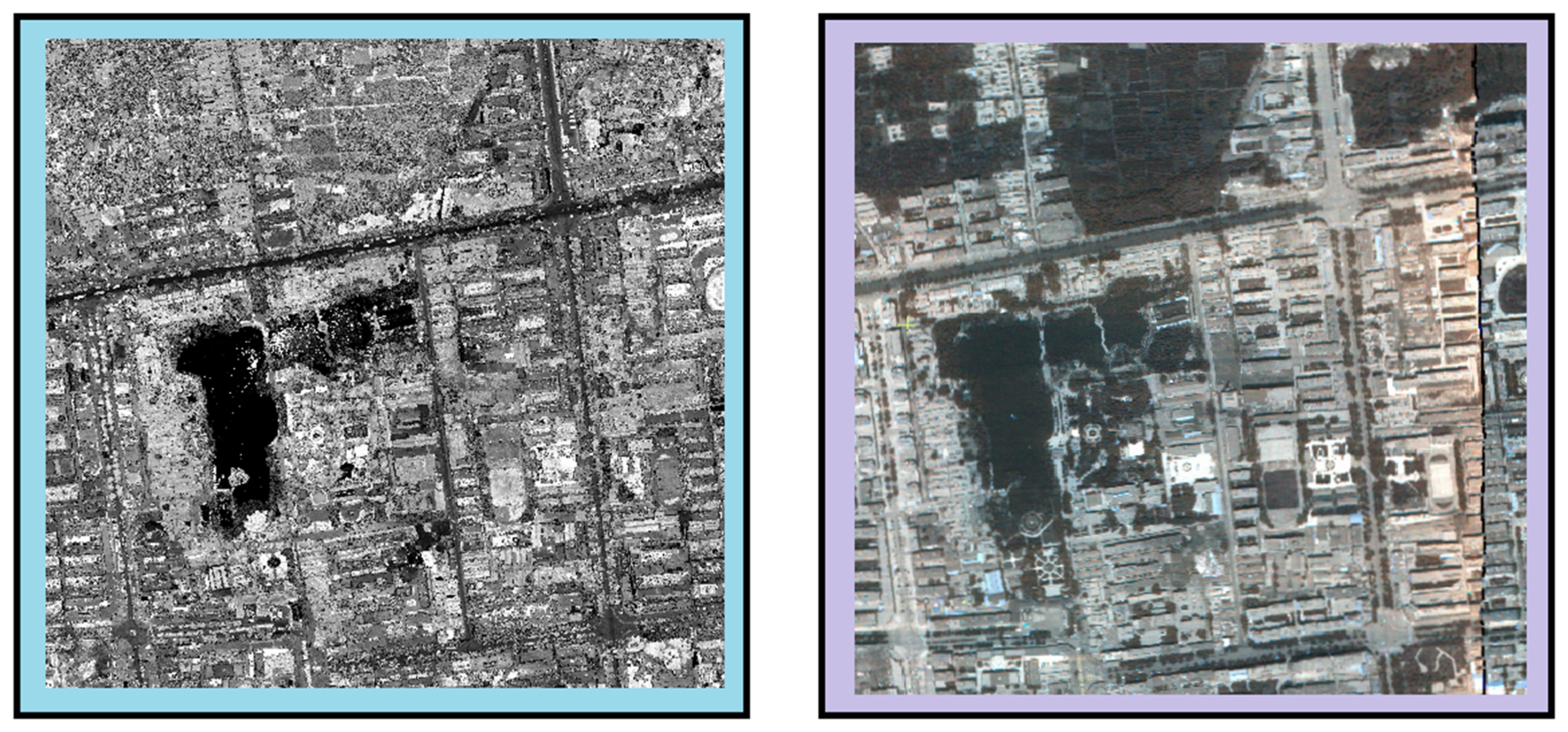
The study area of airborne LiDAR data covered nearly one square kilometer and contained a variety of features, such as trees, houses, tall buildings, roads, vehicles, and streetlights (Figure 5). The trees were distributed in a variety of types, ranging from small forests in the park to relatively sparse street and landscape trees. This dataset was used to validate our method in large-scale urban areas with low-density point cloud data.

2.5.2. UAV LiDAR Data

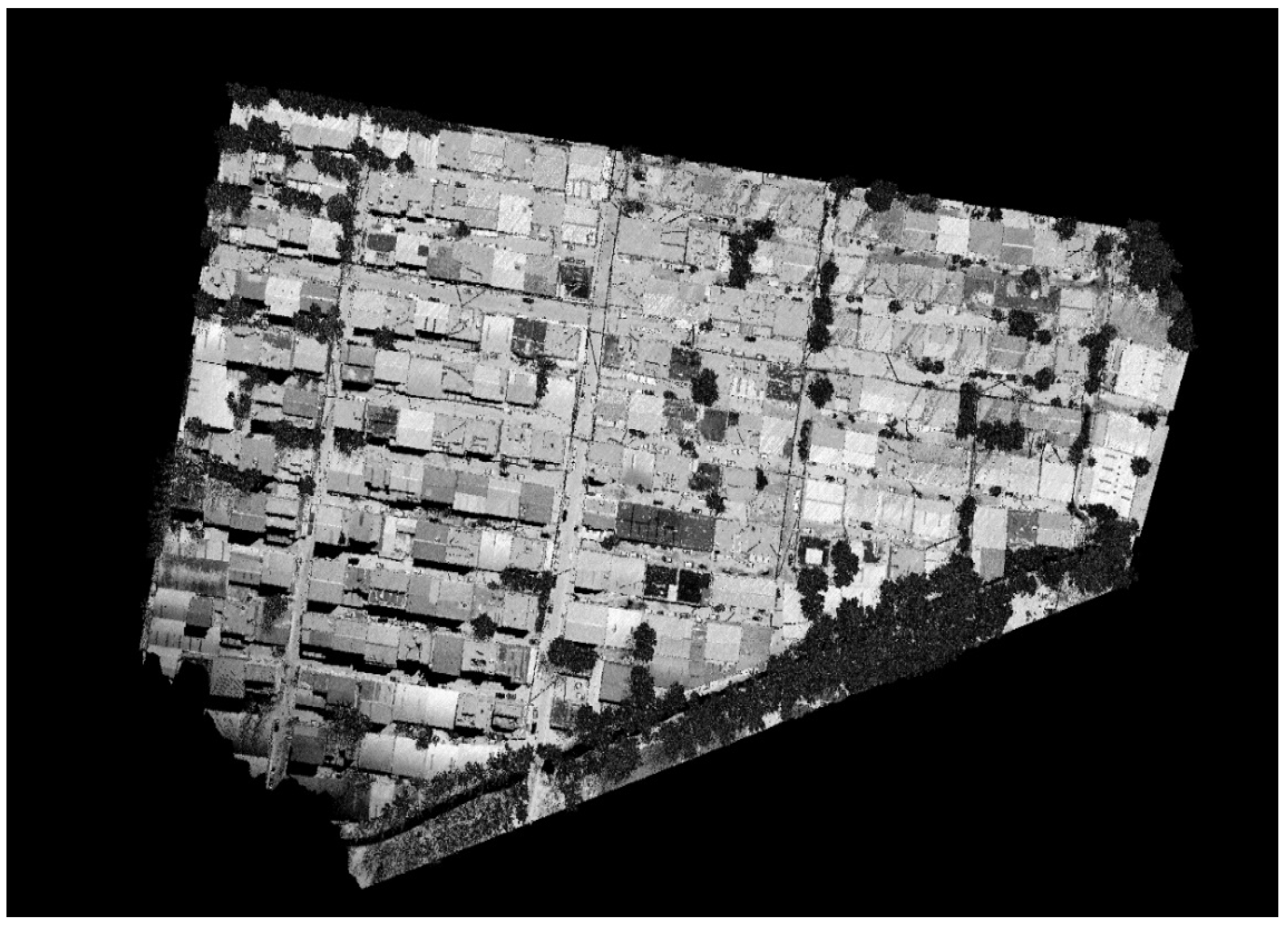
UAV LiDAR data were scanned from Xinyang, Henan, China in March 2021, using a RIEGL VUX-120 (RIEGL Laser Measurement Systems GmbH, Horn Austria) at an altitude of 300 m. The point cloud density was about 165 points per square meter. To be consistent with the airborne LiDAR data, we only used spatial coordinate information. The main objects in this area were roads, power lines, flat-roofed buildings, and trees (Figure 6). This area had a large number of trees in close proximity to houses, power lines, and other features, making the scene correspondingly more complex. This dataset was used to evaluate our method on high-density point cloud data.

3. Results

3.1. Tree Extraction in Airborne LiDAR Data

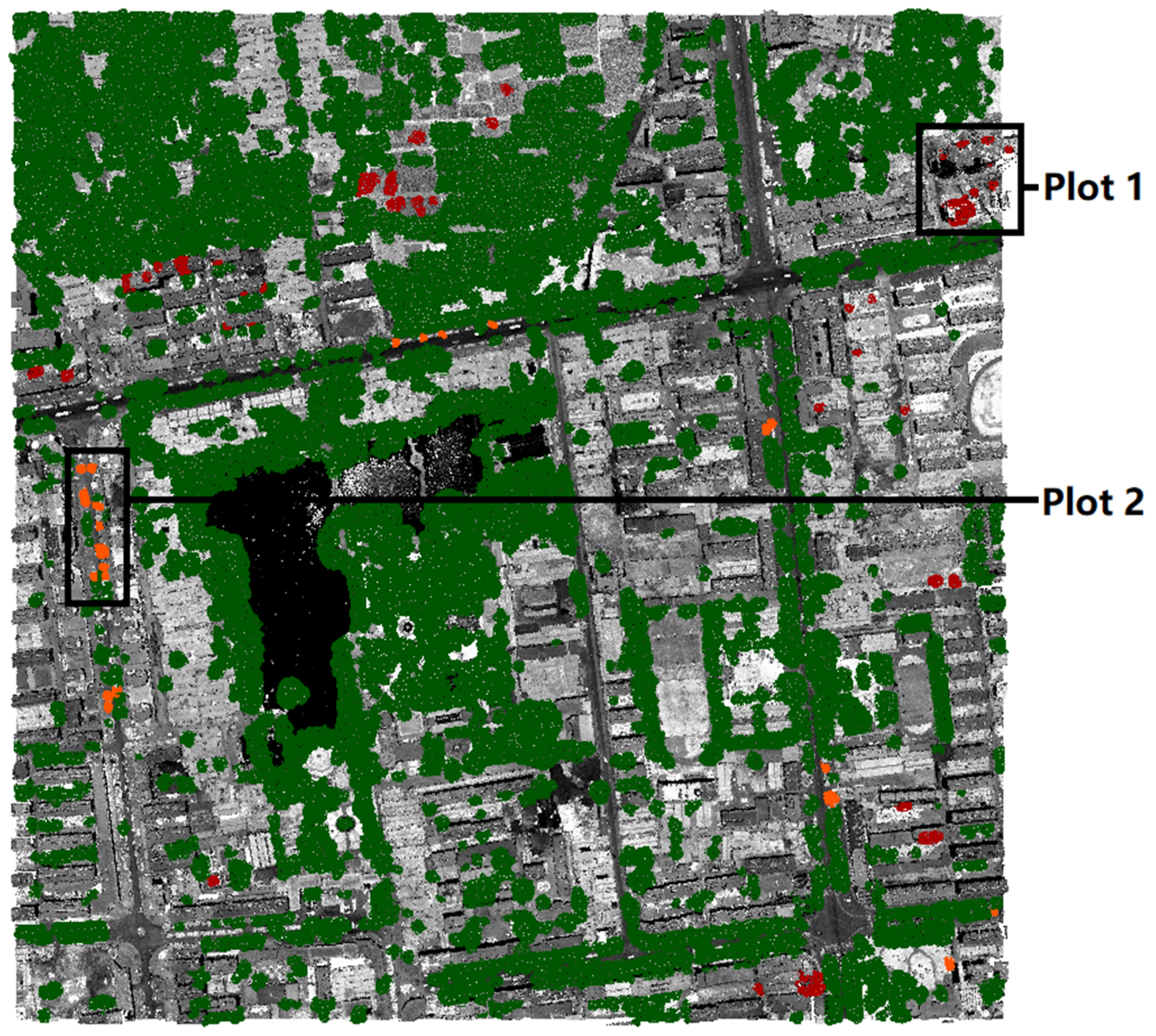
The extraction result is shown in Figure 7. The confusion matrix of our result is given in

Table 2. Confusion matrix for airborne LiDAR data extraction results.

Airborne LiDAR Data	Tree Points (Predicted)	Non-Tree Points (Predicted)
Tree points (Actual)	1,058,408	3979
Non-tree points (Actual)	9208	1,415,515

.

As shown in Figure 7, most trees were both accurately detected and successfully extracted in the study area, in particular, street trees and clustered woods. By analyzing the confusion matrix of the airborne LiDAR data extraction results (Table 2), an accuracy of 0.9947 was achieved, with a precision rate of 0.9914 and a recall rate of 0.9963. This means that most of the tree points are correctly extracted, with only a few non-tree points among the extracted tree points. Although most trees were extracted accurately in the study area, some mis-extracted areas and missing trees were noticed. The uneven facades in the middle of a tall building were likely to be determined as being part of the canopy due to the large difference in height (Figure 8). Some street trees have been pruned with a very flat and small canopy, which our method may have mistakenly filtered out and misjudged as ground or flat roof points (Figure 9).

3.2. Tree Extraction in UAV LiDAR Data

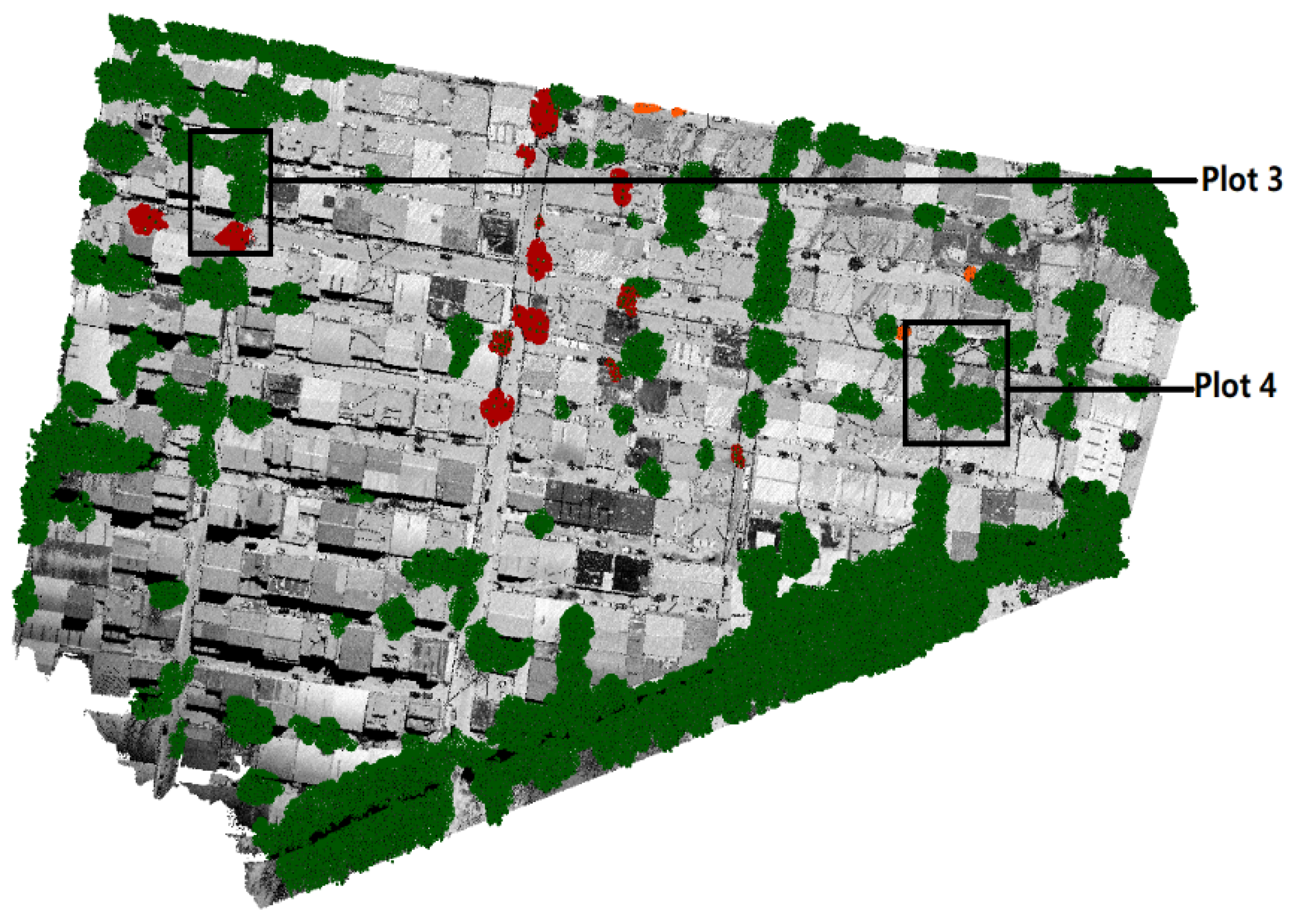
For the UAV LiDAR data, the extraction result is shown in Figure 10, and the confusion matrix of the results is summarized in

Table 3. Confusion matrix for UAV LiDAR data extraction results.

UAV LiDAR Data	Tree Points (Predicted)	Non-Tree Points (Predicted)
Tree points (Actual)	5,196,268	15,895
Non-tree points (Actual)	124,905	12,314,421

.

As shown in Figure 10, most trees were accurately detected and successfully extracted in the UAV LiDAR scanned area. The extraction rate was roughly comparable to that of the airborne LiDAR data, despite the different scene, point cloud density and tree species. The accuracy was 0.9920, with a precision rate of 0.9765 and a recall rate of 0.9970. Despite the higher point cloud density of the UAV data, the precision was slightly reduced compared to that of the airborne data. However, the results indicate that our method had excellent robustness for data with different point-cloud densities.

4. Discussion

With the development of fixed and rotary-wing UAV platforms and improvements in LiDAR technology, the point cloud density of airborne LiDAR data has increased, from a few square meters [52] in the past, to several hundred or even thousand points per square meter, nowadays [53]. With the high density of LiDAR points, data redundancy [54], storage, and the computational burden have become urgent problems [55]. Tree point clouds are only a part of the ground point clouds in urban areas. Most of the methods of extracting tree structure parameters suffer from the weakness of excluding interferences in complex environments, such as buildings and roads in the city. Therefore, the extraction of trees in point cloud data is prior to works like individual tree segmentation or structure parameter retrieval.

4.1. Point Density

In this paper, we proposed a novel approach, based on the morphological characteristics of trees, for the extraction of tree points from urban area point clouds. The results were both surprisingly good on airborne and UAV platforms, which captured very different densities of point clouds. The results revealed that our method worked well, even in areas where buildings and trees intersect, which have been difficult to extract accurately using raster-based methods. Y. Wang et al. found that for individual tree detection, the extracted results for dominant trees were fairly good when the point cloud density was around 2 points/m² [43], which was consistent with our results in airborne LiDAR data. In our tests, densities of 2.5 points per square meter were obtained with an accuracy of up to 99.47%, which was perfectly adequate for most tree extraction requirements. However, Wang et al. pointed out that accuracy would increase with the point density of the data [43], which is contradictory to our results.

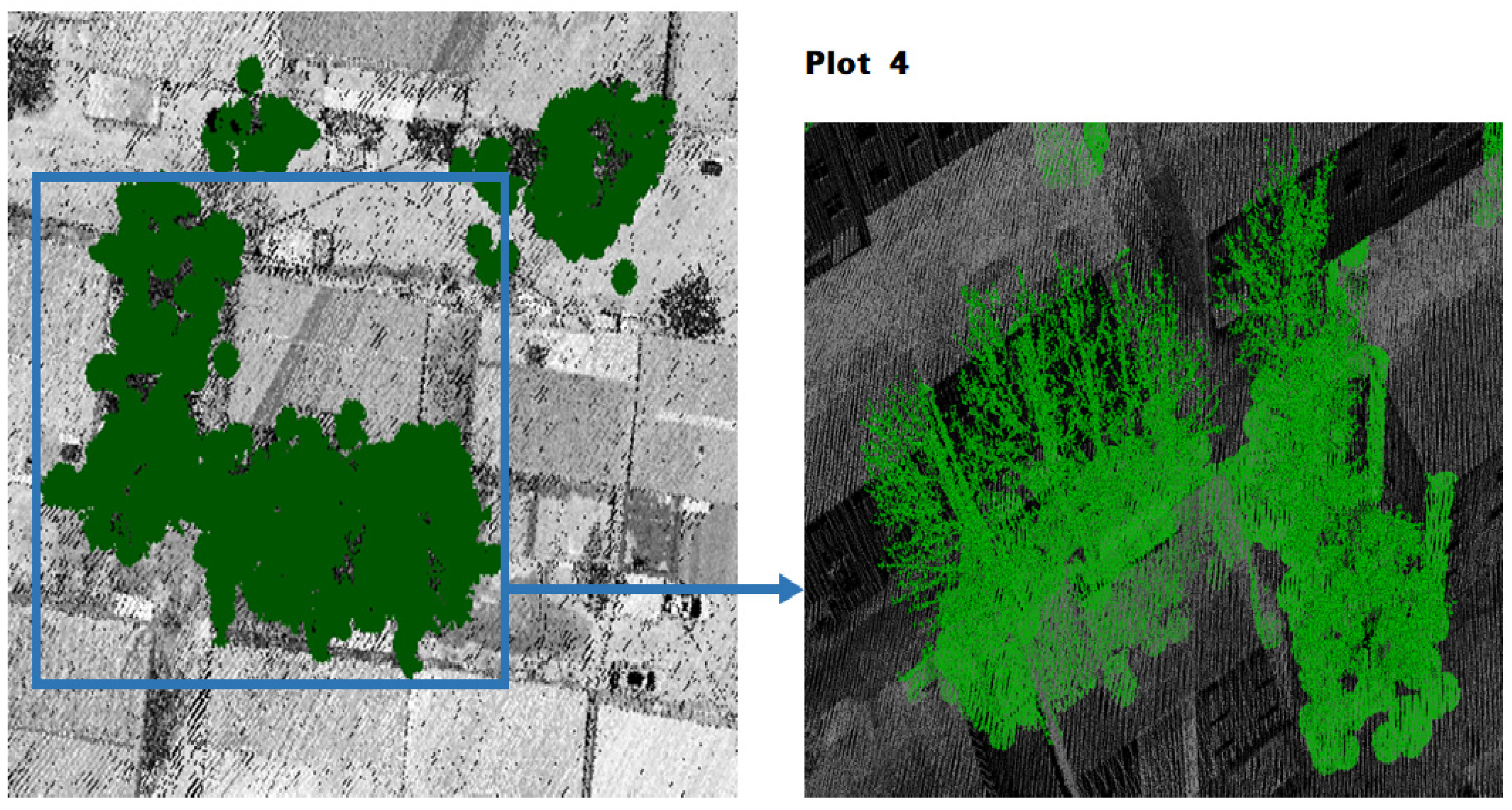
The UAV data’s point density is dozens of times higher than that of ALS. In particular, detailed structures, such as tree branches, are visible in point clouds. In this case, the canopy can no longer be simply considered as a semi-ellipsoid surface but instead as a far more complex structure including branches and leaves. Therefore, we believe that there is not always a positive correlation between point density and the accuracy of extraction results, without changing the algorithm. In our case, this excessive point cloud density also brought us more overhanging interference terms. The most representative challenges in the UAV dataset were power lines. Intricate wires intertwined around poles can easily be misinterpreted as tree canopies (see the blue box in Figure 11), and the vast majority of false extractions in the UAV dataset were brought about by wires intertwined around poles. But encouragingly, experiments have shown that our method is still effective in distinguishing trees from building edges and cars at this fine scale. There were some extremely complex scenes in the UAV dataset, such as dense trees clinging to buildings, parked cars, and protruding balconies (blue box in Figure 12). Extraction results showed that, although trees in UAV LiDAR data are no longer canopy profiles but instead are full of details, such as branches and leaves, they are still well extracted.

4.2. Canopy Structure

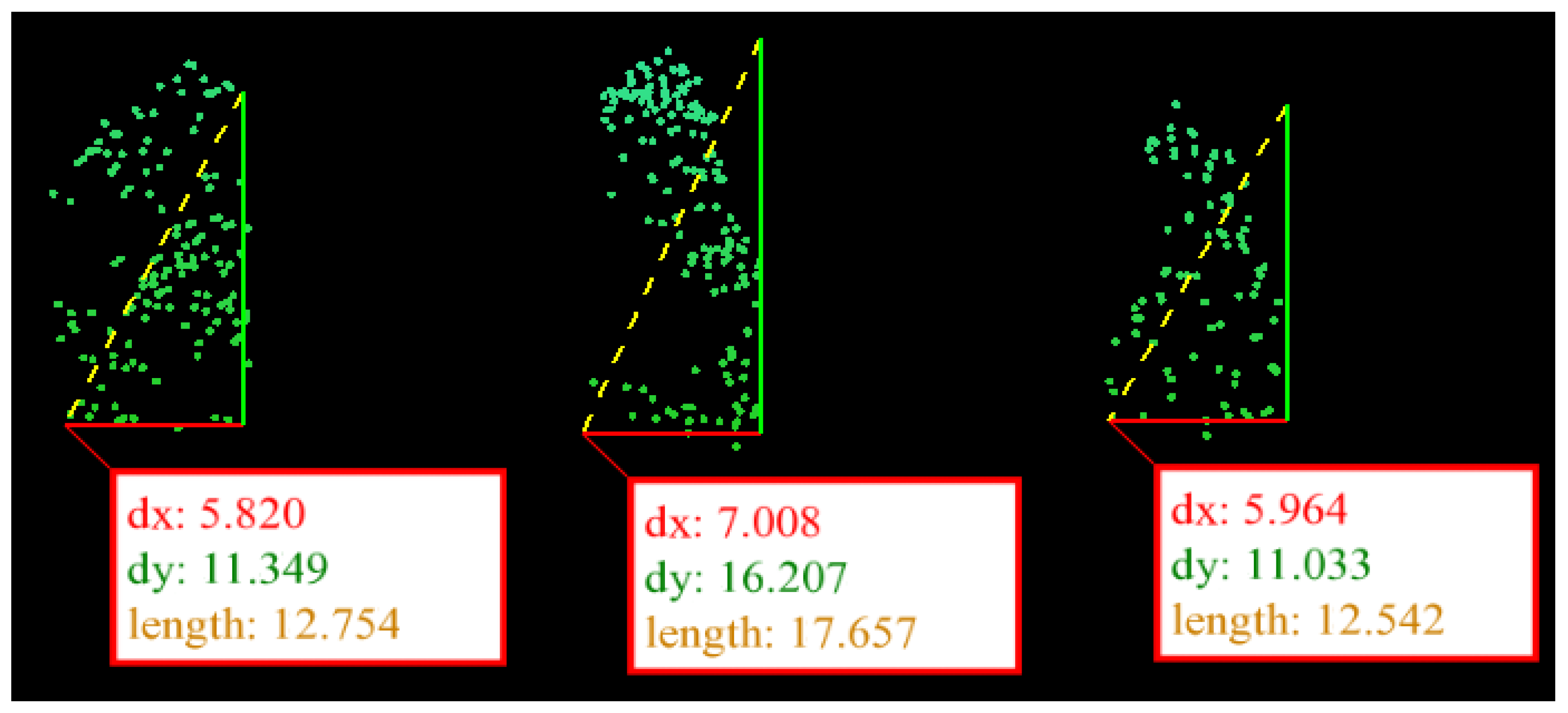
According to our method, trees are likely to be misidentified in two steps: one is when they are filtered out in the first step because they are considered to be flat area points due to their flat canopies, and one is when they are filtered out in the second step because they are treated as features, such as utility poles, due to their small canopy sizes. To figure out whether the missing trees were due to a dominant factor of canopy size or canopy shape, we took the airborne LiDAR data as an example for a further check. By studying the missing trees, we found that all the missing trees were isolated and most of them were street trees that had been pruned artificially. According to our flowchart, pruned trees with a flatter canopy tend to be recognized as part of the ground or as a flat roof in the first step of our method. Just as expected, the missing ones were indeed the trees that had been cut down to a flat crown profile (Figure 13). In addition, we also found several isolated trees whose canopy sizes were relatively small but had significantly undulating upper surfaces (Figure 14). By checking the extraction result, we discovered that they could be extracted correctly. It is abundantly clear that the crown width of the missed trees is far greater than the isolated trees, but that they have flatter crowns. If we use the canopy height (dy in the figure,) divided by the canopy width (dx in the figure), as a simple metric for evaluating canopy undulation, we find that the tree in Figure 13 yields a much smaller value than the tree in Figure 14. Therefore, we can conclude that the problem of missing trees in our morphology-based tree extraction method was mainly dominated by the undulation of the tree canopy. The study by Wang et al. also found that for individual tree detection methods, forest structure was the main factor in determining the accuracy of the results [43]. Therefore, methods such as holistic morphological perception, conducting a more detailed study of the overall morphology of the tree, in the hope of remedying this deficiency will be considered in future works.

4.3. Other Points’ Number—OPN

Since our method uses morphological features to extract trees at the point scale, we only need to use the spatial coordinate information of the point-cloud data. Dispensing with the dependence on echo intensity and multiple sources of data, our method is less affected by the environment, the time of day, and flight altitude during data acquisition.

Although ALS technology has been used in forest inventories for more than a decade, the point-based method is still in a nascent stage and has not yet fully explored the application of morphological feature information [43]. In the process of collecting and identifying morphological features of points by using spatial coordinate information, it is inevitable to set a series of thresholds. In most cases, the final accuracy of the extracted result is strongly correlated with the settings of these thresholds. Morphology-based methods suffer from the uncertainty of the optimal parameter setting [12]. In other words, the previous methods based on morphology failed to extract effectively for diverse scenes using similar thresholds, and it was hard to guarantee high accuracy since the optimal thresholds are hard to determine. By applying the same empirical thresholds to different scenarios, our experimental results showed that most of the thresholds of our method are not very sensitive to the scenarios. However, the parameter OPN in the second step has a high sensitivity to the point density. As the point density of the data increases, the number of points contained in a canopy of the same size increases accordingly. According to our theory, it can be deduced that the theoretical maximum value of OPN is positively correlated with the point density of the data. It is noteworthy that the value of OPN is also highly related to the value of ${\mathrm{R}}_{search}$: a larger ${\mathrm{R}}_{search}$ means a larger search area and larger upper limit of the OPN, whereas a smaller R means a smaller OPN; when ${\mathrm{R}}_{search}$ tends to be 0, the OPN would be fixed at 0. This indicates that it is only when R takes a value greater than a certain value that the OPN can be guaranteed to be meaningful. However, when ${\mathrm{R}}_{search}$ is too large, the features of the local region will be replaced by those of the overall region, and the consequent increase in time complexity will also bring disadvantages to the implementation of the method. Considering that our extraction targets are trees, the value of ${\mathrm{R}}_{search}$ is generally considered to be taken at the same order of magnitude as the tree canopy radius. In addition, in view of the fact that the tree canopy radii do not vary greatly, the value of ${\mathrm{R}}_{search}$ does not need to be changed for most scenarios. Therefore, by controlling the OPN, we can expect to have enough control over the results of the coarse extraction.

4.4. Time Complexity

The time complexity of our method is surmised to be o(n²), and an experiment was run on a computer with a CPU of lntel (R) Core (TM) i9-10900X and a system of Windows 10 to testify our assumption. C++ language and Dev-C++ 5.11 compilation software were used. The time needed for tree point extraction, using our method, for five samples picked arbitrarily and with different point counts, is shown in

Table 4. Time consumption for the data processing of the five samples.

Sample No.	Point Count	Time(s)
1	31,779	12.28
2	15,818	3.399
3	18,424	4.286
4	184,361	398.3
5	187,941	420

.

From Table 4 we can assume that the time complexity can be taken as $\mathrm{o}\left({\mathrm{n}}^2\right)$, which is unfavorable for large datasets while using our methods for tree extraction. Nevertheless, by reducing the number of points involved in each operation—that is, by “chunking” the original data—the time complexity of the whole process can be lessened to $\mathrm{o}\left(\mathrm{m}\ast \mathrm{n}\right)$, where n represents the point count of the original data and m represents the average point count of the chunks.

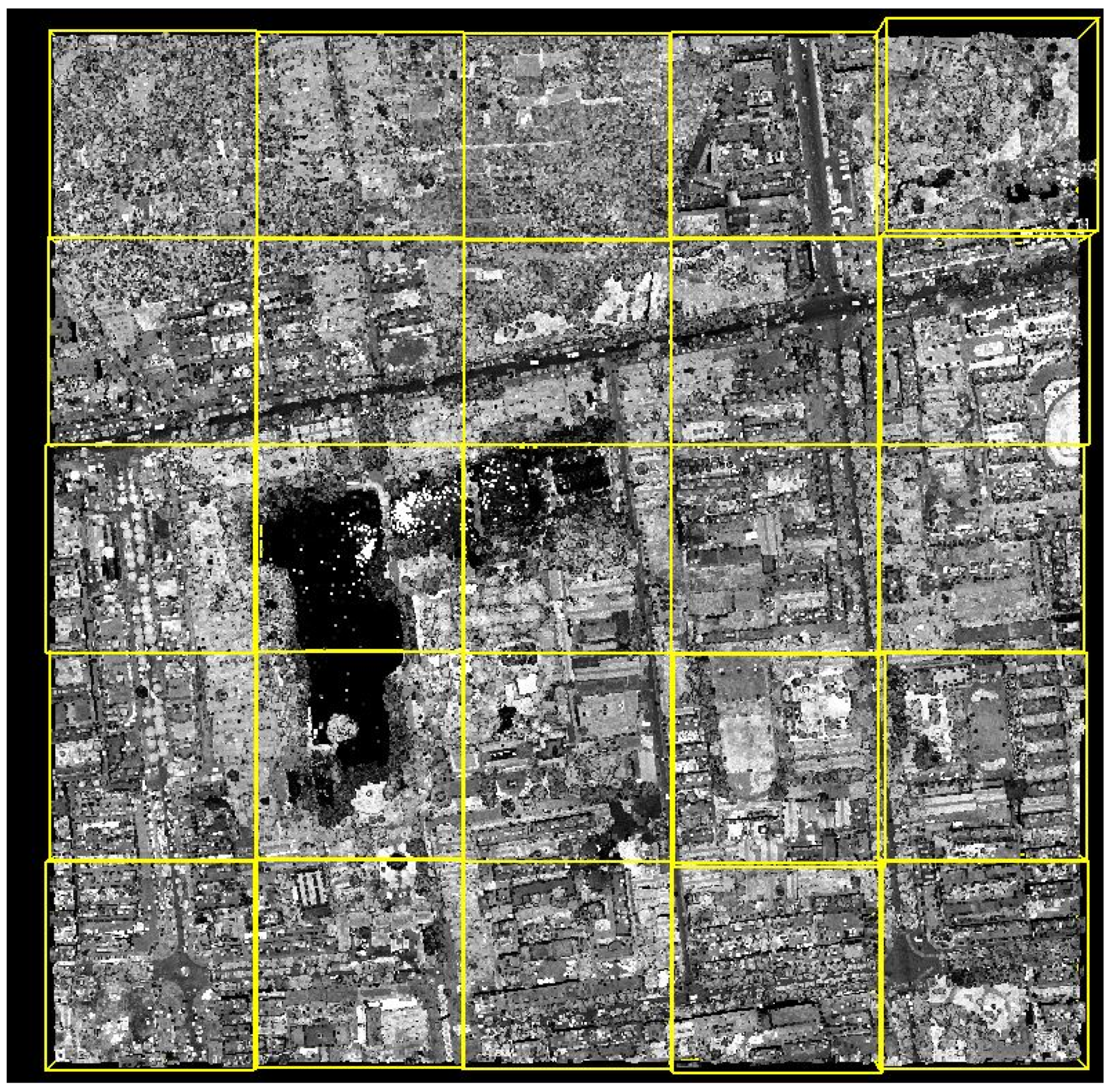
Taking the airborne LiDAR data as an example, we divided it into 25 chunks, with an area of 4 hectares each, in the pre-processing session (Figure 15). The time consumptions of the chunks are shown in

Table 5. Time consumption for airborne LiDAR data processing.

Chunk No.	Point Count	Time for Ground and Flat-Roof Point Removal (s)	Time for Coarse Extraction (s)	Time for Fine Extraction (s)
1	96,431	139.3	0.1636	2.486
2	103,393	157.2	0.3221	4.115
3	86,857	116.9	0.4495	4.563
4	93,904	133.9	0.4415	4.833
5	108,370	173.0	0.3749	5.059
6	98,016	144.4	0.1847	2.402
7	87,571	118.5	0.9525	6.088
8	104,104	161.1	0.6637	6.805
9	105,428	165.0	0.4308	5.213
10	116,034	193.7	0.5291	6.476
11	106,838	171.4	0.5035	5.755
12	60,882	67.5	1.0400	4.267
13	105,461	164.2	1.1700	8.251
14	111,570	182.9	0.2320	3.663
15	108,180	172.8	0.2170	3.160
16	105,307	164.4	0.5126	5.868
17	101,178	152.2	0.6608	6.153
18	108,810	173.7	2.3400	10.740
19	105,804	166.4	0.3484	4.601
20	96,951	142.4	0.2378	3.098
21	98,828	146.7	1.8070	7.540
22	100,058	164.3	0.6765	5.981
23	82,548	106.9	1.1220	6.358
24	94,422	134.7	0.3687	4.586
25	100,165	148.1	0.9651	7.466

. It can be derived that the processes of ground and flat-roof removal are the most time-consuming, while the process of coarse extraction is always quite fast. Since the coarse extraction can already bring us many tree points, the number of iterations for fine extraction is correspondingly reduced significantly, making the process efficient. Using the same computer that was used to test for the time complexity above, the total time required for tree extraction of the ALS data was about 65 min, which is acceptable when dealing with urban datasets. Furthermore, we consider that the operations of each part after chunking are independent; hence, multi-threading techniques can be used to accelerate processing in the future. In addition, special data structures such as octree can eliminate the need for traversal during operations, leading to faster program performance. This, however, would also pose the drawback of increasing the space complexity.

5. Conclusions

This paper proposed a new point-based method for tree extraction, using ALS point cloud data in urban areas, by redefining the flat areas and using the 3D morphological features of trees. Our method needs only the X, Y, and Z coordinates of each point, and has good compatibility with data having different point densities. In addition, this method is easy to use and robust enough for complex scenes with only one parameter to guarantee its effectiveness. We examined the method for both airborne LiDAR data and UAV data in urban areas. The achieved accuracy was 99.4% and 99.2%, respectively. Through further analysis, we found that the vertical structure of the tree canopy was the dominant factor for the missing trees of our algorithm. Although there are still some limitations when extracting trees with flat canopies, this does not prevent the widespread application of our method for urban tree extraction. Moreover, through chunking and multi-threading, we can significantly reduce the time needed by our method in processing large datasets. Future work will be dedicated to the optimization of our method and flowchart to identify flat-crown trees and determine the optimized value of the parameters automatically.

References

1. Roy, S.; Byrne, J.; Pickering, C. A systematic quantitative review of urban tree benefits, costs, and assessment methods across cities in different climatic zones. Urban For. Urban Green. 2012, 11, 351–363. [Google Scholar] [CrossRef] [Green Version]
2. Phillips, C.; Atchison, J. Seeing the trees for the (urban) forest: More-than-human geographies and urban greening. Aust. Geogr. 2018, 51, 155–168. [Google Scholar] [CrossRef]
3. Wu, B.; Yu, B.; Yue, W.; Shu, S.; Tan, W.; Hu, C.; Huang, Y.; Wu, J.; Liu, H. A Voxel-Based Method for Automated Identification and Morphological Parameters Estimation of Individual Street Trees from Mobile Laser Scanning Data. Remote. Sens. 2013, 5, 584–611. [Google Scholar] [CrossRef] [Green Version]
4. Xiao, Q.; McPherson, E.G. Rainfall interception by Santa Monica’s municipal urban forest. Urban Ecosyst. 2002, 6, 291–302. [Google Scholar] [CrossRef]
5. Klingberg, J.; Konarska, J.; Lindberg, F.; Johansson, L.; Thorsson, S. Mapping leaf area of urban greenery using aerial LiDAR and ground-based measurements in Gothenburg, Sweden. Urban For. Urban Green. 2017, 26, 31–40. [Google Scholar] [CrossRef]
6. Kumar, L.; Mutanga, O. Remote Sensing of Above-Ground Biomass. Remote. Sens. 2017, 9, 935. [Google Scholar] [CrossRef] [Green Version]
7. Zhang, Y.; Shao, Z. Assessing of urban vegetation biomass in combination with LiDAR and high-resolution remote sensing images. Int. J. Remote Sens. 2021, 42, 964–985. [Google Scholar] [CrossRef]
8. Brandt, M.; Tucker, C.; Kariryaa, A.; Rasmussen, K.; Abel, C.; Small, J.; Chave, J.; Rasmussen, L.; Hiernaux, P.; Diouf, A.; et al. An unexpectedly large count of trees in the West African Sahara and Sahel. Nature 2020, 587, 78–82. [Google Scholar] [CrossRef]
9. Lefsky, M.; Cohen, W.; Parker, G.; Harding, D. Lidar Remote Sensing for Ecosystem Studies. BioScience 2009, 52, 19–30. [Google Scholar] [CrossRef]
10. Faridhosseini, A. Using Airborne Lidar to Differentiate Cottonwood Trees in a Riparian Area and Refine Riparian Water Use Estimates; The University of Arizona: Tucson, AZ, USA, 2006. [Google Scholar]
11. Feng, X.; Li, P. A tree species mapping method from UAV images over urban area using similarity in tree-crown object histograms. Remote Sens. 2019, 11, 1982. [Google Scholar] [CrossRef] [Green Version]
12. Yang, H.; Chen, W.; Qian, T.; Shen, D.; Wang, J. The Extraction of Vegetation Points from LiDAR Using 3D Fractal Dimension Analyses. Remote Sens. 2015, 7, 10815–10831. [Google Scholar] [CrossRef] [Green Version]
13. Alonzo, M.; Bookhagen, B.; Roberts, D.A. Urban tree species mapping using hyperspectral and lidar data fusion. Remote Sens Environ. 2014, 148, 70–83. [Google Scholar] [CrossRef]
14. Matasci, G.; Coops, N.C.; Williams, D.A.; Page, N. Mapping tree canopies in urban environments using airborne laser scanning (ALS): A Vancouver case study. For. Ecosyst. 2018, 5, 1–9. [Google Scholar] [CrossRef] [Green Version]
15. Man, Q.; Dong, P.; Yang, X.; Wu, Q.; Han, R. Automatic Extraction of Grasses and Individual Trees in Urban Areas Based on Airborne Hyperspectral and LiDAR Data. Remote Sens. 2020, 12, 2725. [Google Scholar] [CrossRef]
16. Plowright, A.A.; Coops, N.C.; Eskelson, B.N.; Sheppard, S.R.; Aven, N.W. Assessing urban tree condition using airborne light detection and ranging. Urban For. Urban Green. 2016, 19, 140–150. [Google Scholar] [CrossRef]
17. Wang, Y.; Jiang, T.; Liu, J.; Li, X.; Liang, C. Hierarchical Instance Recognition of Individual Roadside Trees in Environmentally Complex Urban Areas from UAV Laser Scanning Point Clouds. ISPRS Int. J. Geo-Inf. 2020, 9, 595. [Google Scholar] [CrossRef]
18. Wehr, A.; Lohr, U. Airborne laser scanning—an introduction and overview. ISPRS J. Photogramm. Remote Sens. 1999, 54, 68–82. [Google Scholar] [CrossRef]
19. Chen, Y.; Wang, S.; Li, J.; Ma, L.; Wu, R.; Luo, Z.; Wang, C. Rapid urban roadside tree inventory using a mobile laser scanning system. IEEE J. Sel. Top. Appl. Earth Obs. Remote Sens. 2019, 12, 3690–3700. [Google Scholar] [CrossRef]
20. Li, S.; Dai, L.; Wang, H.; Wang, Y.; He, Z.; Lin, S. Estimating Leaf Area Density of Individual Trees Using the Point Cloud Segmentation of Terrestrial LiDAR Data and a Voxel-Based Model. Remote Sens. 2017, 9, 1202. [Google Scholar] [CrossRef] [Green Version]
21. Su, Z.; Li, S.; Liu, H.; Liu, Y. Extracting Wood Point Cloud of Individual Trees Based on Geometric Features. IEEE Geosci. Remote Sens. Lett. 2019, 16, 1294–1298. [Google Scholar] [CrossRef]
22. Xu, Y.; Li, S.; You, H.; He, Z.; Su, Z. Retrieval of Canopy Gap Fraction From Terrestrial Laser Scanning Data Based on the Monte Carlo Method. IEEE Geosci. Remote. Sens. Lett. 2021, PP, 1–5. [Google Scholar] [CrossRef]
23. Xu, S.; Xu, S.; Ye, N.; Zhu, F. Automatic extraction of street trees’ nonphotosynthetic components from MLS data. Int. J. Appl. Earth Obs. Geoinf. 2018, 69, 64–77. [Google Scholar] [CrossRef]
24. Husain, A.; Vaishya, R.C. Detection and thinning of street trees for calculation of morphological parameters using mobile laser scanner data. Remote. Sens. Appl. Soc. Environ. 2018, 13, 375–388. [Google Scholar] [CrossRef]
25. Guan, H.; Yu, Y.; Ji, Z.; Li, J.; Zhang, Q. Deep learning-based tree classification using mobile LiDAR data. Remote. Sens. Lett. 2015, 6, 864–873. [Google Scholar] [CrossRef]
26. Szabó, Z.; Schlosser, A.; Túri, Z.; Szabó, S. A review of climatic and vegetation surveys in urban environment with laser scanning: A literature-based analysis. Geogr. Pannonica 2019, 23, 411–421. [Google Scholar] [CrossRef] [Green Version]
27. Höfle, B.; Hollaus, M.; Hagenauer, J. Urban vegetation detection using radiometrically calibrated small-footprint full-waveform airborne LiDAR data. ISPRS J. Photogramm. Remote. Sens. 2012, 67, 134–147. [Google Scholar] [CrossRef]
28. Reitberger, J.; Krzystek, P.; Stilla, U. Analysis of full waveform LiDAR data for the classification of deciduous and coniferous trees. Int. J. Remote Sens. 2008, 29, 1407–1431. [Google Scholar] [CrossRef]
29. Lucas, C.; Bouten, W.; Koma, Z.; Kissling, W.; Seijmonsbergen, A. Identification of linear vegetation elements in a rural landscape using LiDAR point clouds. Remote Sens. 2019, 11, 292. [Google Scholar] [CrossRef] [Green Version]
30. Shao, J.; Zhang, W.; Shen, A.; Mellado, N.; Cai, S.; Luo, L.; Wang, N.; Yan, G.; Zhou, G. Seed point set-based building roof extraction from airborne LiDAR point clouds using a top-down strategy. Autom. Constr. 2021, 126, 103660. [Google Scholar] [CrossRef]
31. Heinzel, J.; Koch, B. Exploring full-waveform LiDAR parameters for tree species classification. Int. J. Appl. Earth Obs. Geoinform. 2011, 13, 152–160. [Google Scholar] [CrossRef]
32. Yu, B.; Liu, H.; Zhang, L.; Wu, J. An object-based two-stage method for a detailed classification of urban landscape components by integrating airborne LiDAR and color infrared image data: A case study of downtown Houston. In Proceedings of the 2009 Joint Urban Remote Sensing Event, Shanghai, China, 20–22 May 2009; pp. 1–8. [Google Scholar]
33. Dai, W.; Yang, B.; Dong, Z.; Shaker, A. A new method for 3D individual tree extraction using multispectral airborne LiDAR point clouds. ISPRS J. Photogramm. Remote. Sens. 2018, 144, 400–411. [Google Scholar] [CrossRef]
34. Ma, Z.; Pang, Y.; Wang, D.; Liang, X.; Chen, B.; Lu, H.; Weinacker, H.; Koch, B. Individual Tree Crown Segmentation of a Larch Plantation Using Airborne Laser Scanning Data Based on Region Growing and Canopy Morphology Features. Remote Sens. 2020, 12, 1078. [Google Scholar] [CrossRef] [Green Version]
35. Yun, T.; Jiang, K.; Li, G.; Eichhorn, M.P.; Fan, J.; Liu, F.; Chen, B.; An, F.; Cao, L. Individual tree crown segmentation from airborne LiDAR data using a novel Gaussian filter and energy function minimization-based approach. Remote Sens. Environ. 2021, 256, 112307. [Google Scholar] [CrossRef]
36. Ke, Y.; Quackenbush, L.J. A review of methods for automatic individual tree-crown detection and delineation from passive remote sensing. Int. J. Remote. 2011, 32, 4725–4747. [Google Scholar] [CrossRef]
37. Hyyppä, J.; Yu, X.; Hyyppä, H.; Vastaranta, M.; Holopainen, M.; Kukko, A.; Kaartinen, H.; Jaakkola, A.; Vaaja, M.; Koskinen, J.; et al. Advances in Forest Inventory Using Airborne Laser Scanning. Remote. Sens. 2012, 4, 1190–1207. [Google Scholar] [CrossRef] [Green Version]
38. Vega, C.; Hamrouni, A.; El Mokhtari, S.; Morel, J.; Bock, J.; Renaud, J.-P.; Bouvier, M.; Durrieu, S. PTrees: A point-based approach to forest tree extraction from lidar data. Int. J. Appl. Earth Obs. Geoinf. 2014, 33, 98–108. [Google Scholar] [CrossRef]
39. Hu, B.; Li, J.; Jing, L.; Judah, A. Improving the efficiency and accuracy of individual tree crown delineation from high-density LiDAR data. Int. J. Appl. Earth Obs. Geoinf. 2014, 26, 145–155. [Google Scholar] [CrossRef]
40. Véga, C.; Durrieu, S. Multi-level filtering segmentation to measure individual tree parameters based on Lidar data: Application to a mountainous forest with heterogeneous stands. Int. J. Appl. Earth Obs. Geoinf. 2011, 13, 646–656. [Google Scholar] [CrossRef] [Green Version]
41. Hyyppa, J.; Kelle, O.; Lehikoinen, M.; Inkinen, M. A segmentation-based method to retrieve stem volume estimates from 3-D tree height models produced by laser scanners. IEEE Trans. Geosci. Remote. Sens. 2001, 39, 969–975. [Google Scholar] [CrossRef]
42. Kwak, D.-A.; Lee, W.-K.; Lee, J.-H.; Biging, G.S.; Gong, P. Detection of individual trees and estimation of tree height using LiDAR data. J. For. Res. 2007, 12, 425–434. [Google Scholar] [CrossRef]
43. Wang, Y.; Hyyppa, J.; Liang, X.; Kaartinen, H.; Yu, X.; Lindberg, E.; Holmgren, J.; Qin, Y.; Mallet, C.; Ferraz, A.; et al. International Benchmarking of the Individual Tree Detection Methods for Modeling 3-D Canopy Structure for Silviculture and Forest Ecology Using Airborne Laser Scanning. IEEE Trans. Geosci. Remote. Sens. 2016, 54, 5011–5027. [Google Scholar] [CrossRef] [Green Version]
44. Zhang, K.; Chen, S.C.; Whitman, D. A progressive morphological filter for removing nonground measurements from airborne LiDAR data. IEEE Geosci. Remote Sens. 2003, 41, 872–882. [Google Scholar] [CrossRef] [Green Version]
45. Sithole, G.; Vosselman, G. The Full Report: ISPRS Comparison of Existing Automatic Filters. Available online: http://www.itc.nl/isprswgIII-3/filtertest/ (accessed on 19 August 2015).
46. Meng, X.; Currit, N.; Zhao, K. Ground filtering algorithms for airborne LiDAR data: A review of critical issues. Remote Sens. 2010, 2, 833–860. [Google Scholar] [CrossRef] [Green Version]
47. Zlinszky, A.; Boergens, E.; Glira, P.; Pfeifer, N. Airborne Laser Scanning for calibration and validation of inshore satellite altimetry: A proof of concept. Remote Sens. Environ. 2017, 197, 35–42. [Google Scholar] [CrossRef] [Green Version]
48. Wu, J.; Yao, W.; Chi, W.; Zhao, X. Comprehensive quality evaluation of airborne lidar data. In Proceedings of the SPIE 8286, International Symposium on Lidar and Radar Mapping 2011: Technologies and Applications, Nanjing, China, 26–29 May 2011; p. 828604. [Google Scholar]
49. Wang, D.; Wang, J.; Scaioni, M.; Si, Q. Coarse-to-Fine Classification of Road Infrastructure Elements from Mobile Point Clouds Using Symmetric Ensemble Point Network and Euclidean Cluster Extraction. Sensors 2019, 20, 225. [Google Scholar] [CrossRef] [PubMed] [Green Version]
50. Pontius, R.G.; Millones, M. Death to Kappa: Birth of quantity disagreement and allocation disagreement for accuracy assessment. Int. J. Remote Sens. 2011, 32, 4407–4429. [Google Scholar] [CrossRef]
51. He, Q.; Ma, M. WATER: Dataset of Airborne LiDAR Mission in the Zhangye-Yingke Flight Zone on Jun. 20 2008; A Big Earth Data Platform for Three Poles: Beijing, China, 2012. [Google Scholar]
52. Axelsson, P. Processing of laser scanner data—algorithms and applications. ISPRS J. Photogramm. Remote. Sens. 1999, 54, 138–147. [Google Scholar] [CrossRef]
53. Webster, C.; Mazzotti, G.; Essery, R.; Jonas, T. Enhancing airborne LiDAR data for improved forest structure representation in shortwave transmission models. Remote. Sens. Environ. 2020, 249, 112017. [Google Scholar] [CrossRef]
54. Almeida, D.; Stark, S.; Chazdon, R.; Nelson, B.; Cesar, R.; Meli, P.; Gorgens, E.; Duarte, M.; Valbuena, R.; Moreno, V.; et al. The effectiveness of lidar remote sensing for monitoring forest cover attributes and landscape restoration. For. Ecol. Manag. 2019, 438, 34–43. [Google Scholar] [CrossRef]
55. Koch, B.; Kattenborn, T.; Straub, C.; Vauhkonen, J. Segmentation of forest to tree objects. In Forestry Applications of Airborne Laser Scanning; Springer: Dordrecht, The Netherlands, 2014; pp. 89–112. [Google Scholar]
Figure 1. Flowchart of tree points extraction method.
Remotesensing 13 03428 g001
Figure 2. (a) One selected flat area; (b) Profile of flat area; (c) Top view of the selected flat area. The road in the study area is considered to be a flat area, but we can still see a maximum height difference of sub-meter levels among the selected road points.
Remotesensing 13 03428 g002
Figure 3. (a) Point-cloud projecting; (b) OPN counting. Points in three-dimensional space (blue ones) are projected onto a two-dimensional plane (orange ones) by only retaining their x and y coordinates. Taking the red pentagram as a center point, with its searching area circled in black, the OPN of the point, marked as the red pentagram, can be counted as 7.
Remotesensing 13 03428 g003
Figure 4. Fine extraction iteration schematic. Orange points represent the points derived from coarse extraction; black points represent the points in S u ; green points represent tree points derived from the fine extraction; and the gray points are the points in the original data that are not involved in the operation. As a result of the iteration, the orange and green points together form the tree points.
Remotesensing 13 03428 g004
Figure 5. Airborne LiDAR data. On the left is a display of the LiDAR point cloud data in Zhangye, Gansu, China, according to its intensity information, and on the right is a CCD aerial image of the corresponding area. In the airborne LiDAR data, there are three main types of trees in terms of their spatial distribution: individual trees, street trees aligned in a row, and trees in a cluster formation.
Remotesensing 13 03428 g005
Figure 6. UAV LiDAR data. The image above is a top view of the UAV LiDAR data in Xinyang, Henan, China in terms of the intensity information.
Remotesensing 13 03428 g006
Figure 7. Tree point extraction results of the airborne LiDAR data. Most trees in the study area are well extracted (green points). Street shrubs with small, flat canopies are more likely missed (orange points). Large balconies and facades of tall buildings are the main components of mis-extractions (red points). Only two representative plots were selected for type I error and type II error, respectively.
Remotesensing 13 03428 g007
Figure 8. The edges of the building that were mistakenly extracted as trees are shown as red points.
Remotesensing 13 03428 g008
Figure 9. Trees that were not extracted (orange points).
Remotesensing 13 03428 g009
Figure 10. Tree point extraction results of the UAV LiDAR data. Most of the trees are successfully extracted (green points). One incomplete tree at the edges of the data and two trees with small canopies are missed in the extraction (orange points). The mis-extractions (red points) are mainly cluttered and overhanging wires.
Remotesensing 13 03428 g010
Figure 11. Building edges with overhanging wires that were mistakenly extracted as trees (red points).
Remotesensing 13 03428 g011
Figure 12. Trees extracted in complex scenes (green points).
Remotesensing 13 03428 g012
Figure 13. Two missing trees (points in orange) with flat canopies.
Remotesensing 13 03428 g013
Figure 14. Three well-extracted trees with small canopy sizes.
Remotesensing 13 03428 g014
Figure 15. Airborne LiDAR data chunking.
Remotesensing 13 03428 g015