Accurate Prediction of Earthquake-Induced Landslides Based on Deep Learning Considering Landslide Source Area

Abstract

An earthquake-induced landslide (EQIL) is a rapidly changing process occurring at the Earth’s surface that is strongly controlled by the earthquake in question and predisposing conditions. Predicting locations prone to EQILs on a large scale is significant for managing rescue operations and disaster mitigation. We propose a deep learning framework while considering the source area feature of EQIL to model the complex relationship and enhance spatial prediction accuracy. Initially, we used high-resolution remote sensing images and a digital elevation model (DEM) to extract the source area of an EQIL. Then, 14 controlling factors were input to a stacked autoencoder (SAE) to search for robust features by sparse optimization, and the classifier took advantage of high-level abstract features to identify the EQIL spatially. Finally, the EQIL inventory collected from the Wenchuan earthquake was used to validate the proposed model. The results show that the proposed method significantly outperformed conventional methods, achieving an overall accuracy (OA) of 91.88%, while logistic regression (LR), support vector machine (SVM), and random forest (RF) achieved 80.75%, 82.22%, and 84.16%, respectively. Meanwhile, this study reveals that shallow machine learning models only take advantage of significant factors for EQIL prediction, but deep learning models can extract more effective information related to EQIL distribution from low-value density data, which is why its prediction accuracy is growing with increasing input factors. There is hope that new knowledge of EQILs can be represented by high-level abstract features extracted by hidden layers of the deep learning model, which are typically acquired by statistical methods.

1. Introduction

Globally, many earthquakes occur annually due to the release of accumulated stress in the Earth’s crust. Catastrophic earthquakes (≥magnitude 6) in mountainous regions could trigger numerous landslides on steep mountain slopes [1,2]. Such earthquake-induced landslides (EQILs) can cause tragic economic losses and human causalities by damaging buildings, critical infrastructures, and the environment. Furthermore, other landslides block rivers to form a dammed lake that is a potential risk for outburst floods and debris flow, threatening people and properties downstream [3,4]. Therefore, it is valuable to describe and predict the spatial distribution of earthquake-induced landslides for the sake of disaster prevention and mitigation [5,6,7].

The occurrences of EQILs are primarily controlled by causative factors, including seismic parameters, topography, lithology, tectonics, and human activities, making the spatial patterns of EQILs complicated [8,9,10]. Thus, predicting where landslides are likely to occur after an earthquake is a challenging task [6,11]. In the past two decades, many predictive models have been developed to identify landslide-prone areas after earthquakes, and these are divided into two general categories: (1) physical- and numerical-based models [12,13,14,15]; (2) susceptibility assessment models [16,17].

The physically based models (PBMs) were deduced from the mechanics of slope-failure initiation and runout. Among those models, pseudostatic analysis was the first proposed, assuming that the earthquake force is a permanent body force added to static limit–equilibrium analysis [18,19]. Although pseudostatic analysis is conceptually simple, selecting a pseudostatic coefficient lacks criteria, and crude assumption always leads to conservative results [20]. Stress–deformation analysis, as an extension of finite-element modeling, was later developed and provided a valuable tool for modeling the static and dynamic deformation of slopes. This method is based on mathematical computation, with the capability to solve physical problems with complex geometries, material properties, and boundary conditions, and it is suitable for critical projects researching the stability of artificial slopes [21]. Soon after its implementation, permanent-displacement analysis—whose complexity is between that of the two methods above—was proposed to estimate seismically driven displacements of landslides, considering landslide as a rigid–plastic body that slides on an inclined plane. The representative models of permanent-displacement analysis are the Newmark model and its variations [22]. Over the past few years, the accuracy of physically based models has been enhanced significantly with improvements in analyzing EQIL mechanisms. However, PBMs require a large number of parameter values, which limits their application in a large geographical area [20].

Later, researchers gradually began exploring susceptibility assessment models (SAM) that could represent a potential relationship between EQIL and causative variables and identify EQIL-prone areas [23]. In recent years, landslide susceptibility models have become increasingly popular due to the fast development of computer technology, geographic information systems (GIS), and data mining [24]. Those models can be divided into two categories: knowledge-driven models that are based on expert knowledge and data-driven models that are based on historical landside inventories and related spatial causative data of landslides [25]. The knowledge-based models utilize expert knowledge to quantitatively express the relationship between the landslide occurrence and causative factors, and they regard the analytic hierarchy process (AHP) as the most representative one [26]. For the data-driven models, many statistical methods and machine learning approaches have been introduced to model the probability of landslide occurrence; these mainly include multivariate logistic regression (MLR), artificial neural networks (ANN) [27], support vector machine (SVM) [28], random forests (RF), and decision tree approaches [29]. Researchers have indicated that data-driven models outperform knowledge-driven models in susceptibility mapping. Data-driven models pave the way for detecting the potential distribution pattern of EQILs, which is difficult when only using the naked eye [11].

However, most of the data-driven models mentioned above are traditional machine learning algorithms that can simply represent a single layer of linear or nonlinear relations between causative factors and landslide occurrence [30]. Therefore, those models can easily be overfitted or become stuck on a local optimum when faced with complex data [31,32]. On the other hand, these landslide prediction models rarely consider the difference between landslide source and accumulation due to a limitation in EQIL inventories that always records an EQIL as points or polygons. In the last decade, many deep learning algorithms have achieved remarkable results in computer vision, speech recognition, and intelligent control of robots, whose capacity for exploiting the potential of multiple relationships in massive data has also been gradually noticed by geohazard specialists [33,34,35,36,37,38]. Consequently, some types of deep learning framework have been successfully applied to landslide detection and prediction, including deep neural networks (DNN), convolution neural networks (CNNs), stacked autoencoder (SAE), and their derivative models [39,40].

In this paper, a deep learning framework that considers landslide source area is proposed for the spatial prediction of EQIL. Then, the EQIL inventory of the Wenchuan earthquake is used as a sample dataset to train and test the proposed approach. A comprehensive comparison with traditional machine learning models, such as MLR, SVM, and decision tree, is carried out.

2. Methods and Methods

As mentioned above, a new deep learning-based framework is applied for spatially predicting EQILs. In this framework, the stacked autoencoder is responsible for extracting the deep distribution features of EQIL that could represent the nonlinear and interacting relationship between causative factors and EQIL occurrence. Then, those extracted features are input into a classifier to identify an EQIL-prone area.

2.1. Background

An autoencoder (AE) is a kind of construction of the neural network that consists of an input layer $x\in R^n$, a hidden layer $t\in R^p$, and an output layer $y\in R^m$ (Figure 1). In the input layer, the value of every unit denotes raw data that are a quantitative description of the object. After encoding and decoding, the raw data are transformed into a feature space, which is more suitable for pattern recognition or classification [41]. In detail, the AE will first map input layer $x$ into latent vector $y$ by the encoding process. Mathematically, this step is formulated as

$$t=f(W_{x}x+b_x)$$

(1)

where $W_x$ denotes the weights of input-hidden layers, $b_x$ denotes bias term, and $f(.)$ is an activation function named Sigmoid y = 1/1 + exp(−x). Then, the value of the output layer is calculated using

$$y=f(W_{y}t+b_y)$$

(2)

where $W_y$ denotes the weights of hidden-output layers and $b_y$ denotes the bias term of hidden and output units.

There are some errors between the input layer and the output layer from constructed AE with randomly initialized parameters. These errors will limit the output layer’s capacity to represent the input layer, causing information loss. Therefore, an unsupervised learning method is used to train parameters $\theta =\{W_x,W_y,b_x,b_y\}$ by minimizing the loss function. For real-valued inputs, MSE is deemed as a suitable loss function, which is written as

$$J(x,y;\theta )=\frac{1}{2n}{\displaystyle \sum _{i=1}^n{(x_i-y_i)}^2}+2\lambda \Omega (W)$$

(3)

$$\Omega (W)={\displaystyle \sum _{j=1}^m{\displaystyle \sum _{k=1}^p{W}_{jk}^2}}$$

(4)

where $\Omega (W)$ denotes a regularization term that could avoid the overfitting problem of the model, such as L2 normalization; $\lambda$ is decay parameter that balances the relative importance of the regularization term and MSE.

With the loss function, the group of parameter $\theta$ is updated by an optimization algorithm, i.e., stochastic gradient descent (SGD), as follows:

$$W^t=W^{t-1}+\eta \frac{\partial J(\theta )}{\partial W}$$

(5)

$$b_x^t=b_x^{t-1}+\eta \frac{\partial J(\theta )}{\partial b_x}$$

(6)

$$b_y^t=b_y^{t-1}+\eta \frac{\partial J(\theta )}{\partial b_y}$$

(7)

where $\eta$ is the learning rate that could also be dynamically adjusted, increasing the iteration number. When the loss function reaches the relative minimum, the weights matrix and bias vectors are set as AE’s optimal parameters in the specified dataset.

A trained AE has the ability to reconstruct the input data by using a hidden layer. The hidden layer is regarded as an abstract feature representing one kind of property of input data. However, a single AE is limited in feature representation, especially when it comes to highly complex data. SAE, constructed with AEs layer by layer, was proposed to generate the deep abstract feature and was expected to enhance data classification performance. SAE is stacked with several AEs, in which every hidden unit of the former is set as input units of the next AE. Thus, the output of the SAE can be expressed as follows:

$$h_k=f^1(f^2(f^3(\dots f^k())))$$

(8)

$$f^1=(W_{1}x+b_1)$$

(9)

where $W_1$ and $b_1$ denote the weight matrix and bias vector of first AE, respectively.

To obtain the SAE with the ability of data identification, there is a classification layer on top of SAE, such as Softmax [42], naive Bayes, and support vector machine (SVM). Consequently, two training processes are conducted to update the parameters. In the first step, the AEs are applied to the unsupervised method to find the optimal parameter of data reconstruction one by one, which is called “greedy layerwise pretraining”. Then, fine-tuning is adopted to train the whole network. In this step, the loss function is deduced based on the difference between the truth label and the predicted one. It is recognized from the introduction above that all the parameters in the framework contribute to the loss function. Therefore, the error backpropagation algorithm and stochastic gradient descent are combined to optimize the loss function.

2.2. Prediction Framework

Through EQIL inventory statistics, many research works have proved that several related factors control the occurrence of EQIL. Based on these conclusions, the traditional prediction models are applied to represent the relationship between related factors and EQIL. However, these models paid more attention to every factor’s contribution, rather than the combined effect of factors, which limited performance in EQIL prediction. Therefore, we propose a deep learning framework considering landslide source area to model the complex relationship and enhance spatial prediction accuracy.

As shown in Figure 2, the raw features, including triggering and predisposing factors, are input to the model after normalization processing to avoid the convergence failure problem. The first feature layer is then deduced by single-layer AE, which represents the raw dataset with minimum information loss. Some pretrained AEs are stacked to generate high-level abstract features layer by layer, and mapping the relationship between related factors and EQIL occurrence, which is so-called “greedy layer-wise training”.

At the top of SAE, a classifier is added to decide the probability as to whether an input pixel belongs to an EQIL. Initially, the classifier without supervised training is unable to specify the label of pixels; thus, a backpropagation algorithm is often employed to fine-tune the whole framework.

Many studies have indicated that a different group of factors influences the occurrence of EQIL, i.e., identifying EQIL could be considered as a multivariate inverse inference problem, where the hidden units are composite indicators of the prediction model. Generally, the number of hidden units is more than a composite indicator for the sake of complete feature extraction. However, more hidden units in the model increase the risk of feature redundancy and decrease its robustness. To limit the overabundance of information extraction, sparse optimization is applied to ensure proper units are encouraged to activate (a unit is supposed as “active” when its output is close to (1)). The loss function of AE is rewritten as follows:

$$J(x,y;\theta )=\frac{1}{2n}{\displaystyle \sum _{i=1}^n{(x_i-y_i)}^2}+2\lambda \Omega (W)+\beta \mathrm{KL}(\rho ||\stackrel{\wedge }{{\rho }_j})$$

(10)

$$\mathrm{KL}(\rho ||\stackrel{\wedge }{{\rho }_j})={\displaystyle \sum _{j=1}^m\rho \log \frac{\rho }{\stackrel{\wedge }{{\rho }_j}}}+(1-\rho )\log \frac{1-\rho }{1-\stackrel{\wedge }{{\rho }_j}}$$

(11)

where $\mathrm{KL}(\rho ||\stackrel{\wedge }{{\rho }_j})$ is the Kullback–Leibler (KL) divergence between a Bernoulli random variable with mean $\rho$ and a Bernoulli random variable with mean $\stackrel{\wedge }{{\rho }_j}$; $\beta$ is the weight of the sparsity penalty term.

$$\stackrel{\wedge }{{\rho }_j}=\frac{1}{m}{\displaystyle \sum _{i=1}^m{a}_j(x^i)}$$

(12)

where $\widehat{{\rho }_j}$ is the average activation of hidden unit $j$ on the training set, $m$ is the number of samples, and $a_j$ denotes activation of hidden unit $j$ based on specified $x^i$.

2.3. Model Evaluation

Predicting EQIL and non-EQIL could be a typical binary classification. Therefore, we apply a confusion matrix to evaluate the performance of the model; as illustrated in

Table 1. Confusion matrix.

	Actually Positive (1)	Actually Negative (0)
Predicted Positive (1)	True Positives (TP)	False Positives (FP)
Predicted Negative (0)	False Negatives (FN)	True Negatives (TN)

, true positive (TP) denotes the number of correct predictions, and false positive (FP) denotes the number of incorrect predictions that should be non-EQIL. On the contrary, false negative (FN) denotes the number of incorrect predictions that should be EQIL, and true negative (TN) denotes the number of correct predictions.

Based on the confusion matrix, overall accuracy (OA), Precision, and Recall are deduced as criteria for performance evaluation, which are written as follows:

$$OA=\frac{TP+TN}{TP+FN+FP+TN}$$

(13)

$$Precision=\frac{TP}{TP+FP}$$

(14)

$$Recall=\frac{TP}{TP+FN}$$

(15)

The OA is the probability that represents whether a sample is correctly classified, calculated by summing the number of corrected predictions and dividing by the total number of samples. Precision is the probability that the predicted EQIL is indeed an EQIL, which is deduced by summing the total number of correctly predicted EQIL examples and dividing by the total number of predicted EQILs. High recall score indicates the EQIL is correctly recognized at good performance, defined as the ratio of correctly predicted EQIL and the number of positive predictions.

3. EQIL Inventory

EQIL inventories are essential datasets for researchers exploring the relationship between earthquakes and landslides. Previously, field investigation has been commonly used to obtain an EQIL inventory, but it is time consuming and incomplete in some remote and inaccessible places. Remote sensing technology’s popularity makes an EQIL inventory more reliable, which significantly extends our knowledge of EQILs by statistical methods [43]. Thus far, more than 300 inventories have been constructed after catastrophic earthquakes that have triggered large numbers of landslides. Among these, more than 60 EQIL inventories have been digitized and spread widely [44]. However, these digital EQIL inventories were collected from remote sensing images of different resolutions, leading to a large variability in detail and data format and lack of uniformity and standardization. In this paper, we chose the detailed Wenchuan EQIL inventory to test the model [45].

3.1. Study Area

The study area includes most regions affected by the Wenchuan earthquake and is located between longitudes 102.614–105.482° E and latitudes 30.507–32.701° N (Figure 3). It is dominated by alpine valleys, with elevation ranging from 432 m to 5993 m, and the slope gradient mainly ranges between 20 and 50°. Meanwhile, the mean annual precipitation is about 800–1400 mm, most of which takes place during the period from June to September [46]. Abundant rainfall has promoted high-density drainage networks, with intense surface erosion.

This area has tectonically active mountain belts, namely the Longmenshan (LMS) thrust belt, which is the boundary zone between the Bayankala block of eastern Tibet Plateau and the Sichuan Basin of South China block. Multistage tectonic events have led to the extremely complex lithology of LMS. Due to tectonic stresses, the rock masses are highly fractured and weathered, and consequently prone to slope instability. Based on GPS, it has been proved that the extrusion of crustal material from the Tibetan Plateau against the rigid blocks of the Sichuan Basin induces deformation at about 1 mm/yr and accumulates stress in the Longmenshan regions. Therefore, there are many stress–release earthquakes on faults, especially on the most active faults, including the Yinxiu-Beichuan Fault, the Maoxian-Wenchuan Fault, the Guanxian-Anxian Fault, and the Pingwu-Qingchuan Fault (Figure 3). On 12 May 2008, the devastating Wenchuan earthquake measured Mw 8.3 according to the China Earthquake Administration (CEA), and it occurred on the Yinxiu-Beichuan Fault. This earthquake caused more than 69,000 deaths and over 370,000 injuries, with 17,393 missing by 25 April 2009.

3.2. Training and Testing Samples

The Wenchuan earthquake triggered numerous landslides that caused serious casualties and property damage, especially in the high-relief mountain area. To explore the distribution patterns and mechanisms of EQILs, many studies focused on constructing the EQIL inventories by remote sensing technology and field surveys. However, those inventories were in the landslide’s various presentation manner, from polygons, centroid points, or top points, which could affect the results of statistical analysis. Further, some EQILs inventories for some earthquakes are inconsistent in number because of different interpretation standards, remote sensing images, and experts. For those reasons, traditional inventories are not suitable for training and testing the proposed model.

In this paper, multisource remote sensing images acquired after the earthquake were used to map landslides, referred to the existing inventory from [45], as shown in Figure 4. The landslides were mapped as polygons that separately document source areas and runout areas, based on image and topographic features (Figure 4b,c) [1]. Only the initiation areas were set as samples for model training and testing. It is worth noting that some small-scale rockfalls also cause scars on the image that confuse the interpretation map. Meanwhile, those small scars can hardly be divided into different parts, which might create errors when predicting results. Thus, we concentrate on landslides with clear shapes and boundaries. In total, 23,029 EQILs were ultimately mapped in the study area.

The proposed model is a pixelwise framework that takes as input a feature vector of an individual pixel. The landslide polygons are converted to raster format data with a spatial resolution of 12.5 m, consistent with the resolution of the digital elevation model (DEM). Then, 8,193,389 pixels represent the whole landslides of the study area, and the same number of non-landslide pixels that are regarded as adversarial samples are randomly generated outside the landslide area. In total, a sample database with 1,638,778 pixels is used to support the proposed framework for learning the distribution pattern of EQIL. To obtain a robust prediction model, the samples are divided into training and testing sets at a ratio of 2:8. Detailed information is depicted in

Table 2. Samples generated from the EQIL inventory of the Wenchuan earthquake.

Category Name	No. of Pixels	No. of Training Samples	No. of Testing Samples
EQIL	819,389	163,877	655,512
Non-EQIL	819,389	163,877	655,512
Total	1,638,778	327,754	1,211,024

.

3.3. Training and Testing Samples

In the past three decades, many studies have taken advantage of statistical methods to analyze the relationship between controlling factors and EQIL. In general, these factors are mainly categorized into six groups: (1) seismic property; (2) topography; (3) geology; (4) soil; (5) hydrology; (6) land use. Considering the limitation of data accessibility and the importance of factors, we select 14 factors as input variables for the model [1,5], as listed in

Table 3. List of data sources used as controlling factors in this study.

Category	Control Factors	Data Type	Data Source
Seismic property	EI—Earthquake intensity	Polygon	China Earthquake Administration (CEA)
	ED—Epicenter directivity	Point
	SRD—Surface rupture directivity	Polyline
	AF—Aftershocks	Point
Topography	DEM (12.5 m resolution)	Raster	Alaska Satellite Facility, USA
	SLO—Slope gradients	Raster
	SLOA—Slope aspect	Raster
	TPI—Topographic position index [47]	Raster
	SC—Slope curvature	Raster
	RER—Relative relief	Raster
Geology	LITH—Lithology	Polygon	China Geological Survey
	FD—Fault direction	Polyline
Hydrology	DR—Distance to rivers	Polyline	Department of Forestry, Sichuan Province
Soil	ST—Soil type	Polygon	Department Natural Resources, Sichuan Province

.

The raw data of controlling factors are different from the format, including raster, polyline, polygon, and point. To overlay all the data together, the raw data of factors are quantized and converted to raster with a spatial resolution of 12.5 m, except for topography factors.

For instance, epicenter directivity is denoted as the following index:

$$E_p=\{\begin{array}{cc}\arctan (\frac{x_p-x_e}{y_p-y_e})& x_p>x_e\mathrm{and}{y}_p>y_e\\ \pi +\arctan (\frac{x_p-x_e}{y_p-y_e})& y_p<y_e\\ 2\pi +\arctan (\frac{x_p-x_e}{y_p-y_e})& x_p<x_e\mathrm{and}{y}_p>y_e\end{array}$$

(16)

where $(x_p,y_p)$ and $(x_e,y_e)$ are the coordinates of the epicenter and a specific pixel.

The direction of surface rupture and fault controls the sliding direction of the landslide. To obtain quantitative input for the model, several steps are conducted to reprocess the raw distribution data of surface rupture and fault. In the first, the fault is cut into subsections that can more accurately describe the changes in direction along the fault. Then, the Thiessen polygon that generates competitive advantage trade areas for each point by creating boundary lines is constructed to determine the affected area of every subsection. The direction of the subsection is ultimately applied to indicate the fault direction of the subregion.

The occurrence of aftershocks is a time series process and has an additive effect on slope failure. Therefore, the aftershocks factor is produced by the kernel density analysis method that generates the raster data to model the influence of aftershocks.

Lithology and soil are polygon data, whose relationship with landslide is defined by the frequency ratio values (FR) method in this study. This indicates a strong correlation between EQIL and controlling factors when the value of FR is greater than 1.

$$I=\frac{L_i/L_t}{A_i/A}$$

(17)

where $L_i$ is the area of landslides in $i$th type, $L_t$ is the total area of landslides, $A_i$ is the area of $i$th type, and $A$ is the total area of the study area.

After the preprocessing mentioned previously, all the factors are acquired as shown in Figure 5.

4. Experiment and Results

Using sample data and control factors, the model was trained and tested to find the optimal model structure and parameters. Then, the proposed model was compared with traditional methods and its performance evaluated. Finally, the advantages of the model in EQIL prediction are discussed in relation to feature extraction and threshold segmentation.

4.1. Framework Setting

Many studies have proved that the structure of a deep learning model has a great influence on prediction results. For different datasets, the model must be analyzed to obtain optimal framework settings. In this study, four kinds of framework setting (including hidden units, hidden layers, learning rate, and number of iterations) were considered.

The number of hidden units is related to model parameters that decide the model’s complexity and whether the model is prone to overfitting. Setting the optimal number of hidden units is challenging, as it is susceptible to many factors, such as the number of input and output features. To obtain the suitable number of hidden units for EQIL spatial prediction, the ascending series in intervals of two are experimented with one by one and then assessed by OA. As shown in Figure 6, it is proven that the 110 hidden units are suitable for representing the dataset and can enhance the performance of EQIL prediction in this study.

The depth of the framework is denoted by the number of hidden layers that map the input features to high-level abstract features that represent the multilayer relationship between EQIL occurrence and its controlling factors. The model then takes advantage of these mapping relationships to assess whether a slope is prone to landslides under an earthquake. For complex target recognition, more hidden layers can properly narrow the “semantic gap”, which is defined as the difference between two kinds of representation systems of one object. However, the controlling factors are a high-level description of EQIL by different aspects compared with other raw data (such as a remote sensing image that just records the features of objects in several channels). It is still necessary to extract more abstract features to learn the pattern of EQIL spatial distribution, and then predict potential EQIL.

Therefore, a group of experiments that are in the same setting, except for the number of hidden layers, is conducted to establish how the final prediction accuracy is affected overall. As shown in Figure 6, the OA initially becomes higher with hidden layers increasing; it then decreases. In conclusion, three hidden layers are considered as an optimal setting in this study.

Learning rate decides the convergence speed in processing parameter optimization and whether the optimization goal is becoming globally optimal. It is influenced by the size of sample data and the gradient of the loss function. We considered several learning rates, including 0.0001, 0.001, 0.01, 0.1, and 0.8, to assess the performance, as shown in

Table 4. Prediction result assessment with different learning rate.

Learning Rate	0.0001	0.001	0.01	0.1	0.8
OA (%)	80.35 ± 0.40	83.03 ± 0.05	83.84 ± 0.10	85.49 ± 0.16	86.72 ± 0.23
Precision (%)	79.85 ± 0.45	81.91 ± 0.07	82.45 ± 0.13	84.14 ± 0.88	85.37 ± 0.96
Recall (%)	81.24 ± 0.65	84.83 ± 0.001	86.02 ± 0.11	87.53 ± 1.25	88.68 ± 1.9

. It is clear that the bigger learning rate is suitable for optimizing the constructed objective function in this study.

The number of iterations determines whether the parametric optimization process of the model converges. Too many iterations will cause the overfitting of the model and reduce its robustness. However, too few iterations will result in the model underfitting and local optimality. Therefore, we searched for the optimal number of iterations through multiple sets of experiments, and the results are shown in Figure 7. In the initial iteration, the loss function converges quickly and then slows down gradually. After 30,000 iterations, the accuracy of the model in the test set and the training set rose asynchronously, indicating that the model reached overfitting. Consequently, for this dataset and model setting, we adopted 30,000 iterations to optimize the model’s parameters.

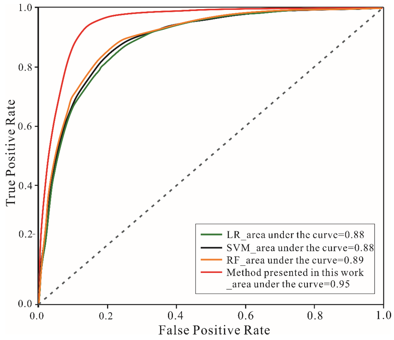
4.2. Visualizing Result and Performance Assessment

After obtaining the optimal settings for the framework, the training and testing samples are used to optimize all parameters and then validate the deep learning framework considering the landslide source area. Three other traditional machine learning algorithms, including logistic regression (LR), support vector machine (SVM) [48], and random forest (RF) [49], are also compared with our methods to analyze their capacity for data mining and EQIL spatial prediction. The LR model constructs the loss function with L2-norm; the regularization coefficient is 1. For SVM, the kernel is radial basis function, the penalty coefficient is 1, and the parameter of kernel function is 0.001. For RF, the number of trees is 62 and the maximum depth is 13.

With the optimal setting, all the methods are trained and tested 20 times to eliminate the influence of random initialization of parameters on evaluation results.

Table 5. Prediction result assessment with different framework depths.

Measurements	Logistic Regression	Support Vector Machine	Random Forest	Proposed Method
OA (%)	80.75 ± 0.23	82.22 ± 0.15	84.16 ± 0.22	91.88 ± 0.18
Precision of EQIL (%)	79.10 ± 0.34	80.70 ± 0.23	81.93 ± 0.17	87.56 ± 0.21
Recall of EQIL (%)	80.33 ± 0.27	82.07 ± 0. 12	84.40 ± 0. 15	91.40 ± 0. 20

lists the OA, Precision, and Recall of the proposed method and other methods. Our method obtains the highest OA value of 91.88%, which is approximately 7% higher than that of RF in second place, followed by SVM and LR, with OA values of 82.22% and 80.75%, respectively. In terms of EQIL prediction precision, the four models are 79.1%, 80.7%, 81.93%, 87.56%, in which our proposed method obtains the highest values. Overall, the deep learning method has the best performance on sample data compared with other shallow machine learning models.

Figure 8 shows the four kinds of predicted result in the whole study area when 0.5 is set as a discrimination threshold of probability. All the results reflect the phenomenon that EQILs distribute along a surface rupture [50]. It can be proved that machine learning models, including shallow models, could learn and apply the basic distribution patterns to predict EQILs spatially. Furthermore, our proposed method has the advantage of elegantly representing EQIL distribution, especially in the north tail of surface rupture and the Wenchuan-Maoxian valley, which require more discriminative features to enhance the model’s prediction ability.

As mentioned above, many shallow machine learning methods have been applied for EQIL spatial predictions, including LR, SVM, decision tree, RF, and AdaBoost. However, these methods depend heavily on the quality of related factors and sample data, whereas the deep learning model is robust for pattern recognition and classification, especially for small sample sizes and highly coarse datasets. We use the trained models to produce the receiver operating characteristic (ROC) curve to validate different EQIL prediction performances between two kinds of machine learning method, as shown in Figure 9. Our method demonstrated the best predictive power compared with other methods in terms of area under the curve (AUC). Specifically, the other three methods obtain similar AUC values of 0.88, 0.88, and 0.89, respectively.

5. Discussion

5.1. High-Level Feature Representation

An EQIL is an extremely complex earth surface process that is controlled by numerous predisposing factors and a triggering event. Analyzing the relationship between factors and EQIL distribution paves the way for recognizing EQIL occurrence and spatial prediction mechanisms. Deep learning as a kind of effective data mining model has been applied in many study areas, and it is well known for its discriminative feature extraction. As shown in Figure 10, the raw features are derived from topographical, geological, and hydrological data, which are then mapped to hidden layers that indicate the controlling effect from different factors. That is to say that a different group of factors is processed by the model and generates a synthetical index related to EQIL occurrence, which is different from traditional methods that consider nearly every related factor contributing to the object separately.

5.2. Performance of Rock Landslide Prediction

A large earthquake (magnitude > 6) can trigger landslides of shallow soil, as well as large, deep rock landslides [51]. A landslide’s initiation is controlled by different failure mechanisms associated with material types, topography, and geotechnical features [52,53,54]. Landslides in bedrock are especially strongly influenced by their structure and preaccumulated failure, which consequently result in complex failure mechanisms compared with soil landslides [55]. Thus, we selected one of the earthquake-affected areas where EQILs were dominated by rock materials to validate our model. As shown in Figure 11, both predictive results from our proposed and FR methods could cover the EQILs from the inventory data. However, FR carries out the final result with several non-EQIL areas, leading to a high false alarm rate. It is proven that the conventional prediction models have a limited capacity for synthetical analysis when faced with a multiple-parameters problem. Therefore, the predictive result from these models is always controlled by the master EQIL-related factors that mathematically have high variance. However, our proposed method could construct high-level abstract features to represent the influence of a combination of different factors on EQIL occurrence and make the spatial prediction more coincident with EQIL distribution.

It is concluded that our deep learning-based model has the potential ability to break through the bottleneck in EQIL predictions. Meanwhile, multilayer feature mapping could help researchers to update the knowledge of landslides that was acquired by statistical methods in the past.

5.3. Influence on Factor Importance

Many studies have confirmed that the initiation of an EQIL is an extremely complex process, indicating why the hazardous assessment and accurate prediction of EQILs have not yet been attempted. Over the years, researchers have introduced a variety of conventional models for EQIL prediction (such as LR, SVM, RF algorithm) and successfully applied them to many EQIL inventories all over the world [44]. Lacking the capacity for deep feature transformation, conventional algorithms usually improve the accuracy of EQIL prediction by selecting high-importance factors to enhance model robustness [11]. However, this data preprocessing method cannot further extract hidden features of coarse and redundant data, and cannot improve the data utilization of EQIL inventories [56]. The coseismic landslide prediction model proposed in this paper is not only superior in terms of data input (extracting sliding features as model input), but also adopts a deep learning model based on a stacked autoencoder. Our proposed accurate prediction framework considering the EQIL source area is not only superior in terms of data input (extracting sliding features as model input), but also introduces SAE to extract the complex features of redundant data. To explain why this model has advantages in terms of EQIL prediction, we conduct several comparative experiments for EQIL distribution with different numbers of controlling factors that have different information contributions, thus reflecting the model’s predictive ability.

First, the information gain function is applied to calculate the feature importance index and rearrange the 14 predisposing factors (Figure 12). As mentioned in [57,58], the information gain function (IG) is one of the quickest and easiest attribute ranking methods that is often used in feature selections and for identifying root nodes in tree-based models. As shown in Figure 12, initially, the prediction performance of all methods improved with the increasing number of input-controlling factors. The prediction accuracies of RF, SVM, and LR remain stable or even decline when the input-controlling factors are greater than seven, which is due to the fact that increasing factors contribute less to EQIL distribution. On the contrary, the proposed method continually obtains better prediction performance. Thus, two points can be concluded: (1) the shallow machine learning models only take advantage of the significant factors for EQIL prediction, but deep learning models can extract more effective information of EQIL distribution from low-value density data, which is why prediction accuracy grows when input factors increase; (2) the EQIL distribution pattern is controlled by a combination of multiple factors; only when the slope unit satisfies specific combination conditions can a landslide be triggered by a catastrophic earthquake. These two conclusions explain why the deep learning model is superior in EQIL prediction, and also provide a hint that some new knowledge of EQIL can be represented by high-level abstract features extracted by the hidden layer of our deep learning model.

6. Conclusions

Earthquakes near human communities can result in significant loss of human life and damage to the environment, especially in high-altitude and steep mountain areas. Meanwhile, earthquakes can trigger many landslides that create secondary geological disasters, increasing the intensity of earthquake damage. Thus, spatially predicting EQILs based on distribution pattern is essential for disaster mitigation. For the last two decades, complete and normalized EQIL inventories have extended our knowledge of the relationship between earthquakes and the landslides they can trigger by means of statistical analysis. However, an effective method to detect new EQIL distribution patterns in large, multiparameter datasets has been lacking, which has limited the performance of EQIL prediction for a long period. Furthermore, the source area features of EQIL, which could well represent predisposing conditions for EQIL occurrence, was seldom taken into consideration in prediction models. Deep learning is known as feature extraction in complex and highly coarse datasets, which could be used to analyze the combinations of different factors that influence EQIL occurrence.

In this study, we constructed a deep learning framework based on the stacked autoencoder (SAE) and considered the source area features of EQILs to model their distribution. The complete EQIL inventory of the Wenchuan earthquake was then applied to assess the performance of the proposed methods. After several controlled experiments, the optimal framework settings (including the number of hidden units, depth of hidden layers, iteration number, learning rate) are 120, 3, 20,000, and 0.8, respectively. Ultimately, the proposed method was compared with traditional prediction models, showing that the deep learning-based model is superior in the spatial prediction of EQILs. Meanwhile, this study reveals that shallow machine learning models only take advantage of the significant factors for EQIL prediction, but deep learning models can extract more effective information about EQIL distribution from low-value density data, which is why its prediction accuracy grows when input factors increase. There is also hope that some new knowledge about EQILs can be represented by high-level abstract features extracted by hidden layers of our deep learning model; these were acquired by statistical methods in the past. In future, our mature EQIL prediction model is expected to be promoted and applied to two scenarios: rapid positioning in the secondary disaster-prone area after an earthquake, based on a basic database, and providing a reference for disaster mitigation, thus creating a risk assessment of potential seismic areas to improve the efficiency of risk management.

References

1. Fan, X.; Scaringi, G.; Korup, O.; West, A.J.; van Westen, C.J.; Tanyas, H.; Hovius, N.; Hales, T.C.; Jibson, R.W.; Allstadt, K.E. Earthquake-induced chains of geologic hazards: Patterns, mechanisms, and impacts. Rev. Geophys. 2019, 57, 421–503. [Google Scholar] [CrossRef] [Green Version]
2. Umar, Z.; Pradhan, B.; Ahmad, A.; Jebur, M.N.; Tehrany, M.S. Earthquake induced landslide susceptibility mapping using an integrated ensemble frequency ratio and logistic regression models in West Sumatera Province, Indonesia. Catena 2014, 118, 124–135. [Google Scholar] [CrossRef]
3. Alfaro, P.; Delgado, J.; García-Tortosa, F.; Lenti, L.; López, J.; López-Casado, C.; Martino, S.J.E.G. Widespread landslides induced by the Mw 5.1 earthquake of 11 May 2011 in Lorca, SE Spain. Eng. Geol. 2012, 137, 40–52. [Google Scholar] [CrossRef]
4. Cui, P.; Zhu, Y.-Y.; Han, Y.-S.; Chen, X.-Q.; Zhuang, J.-Q. The 12 May Wenchuan earthquake-induced landslide lakes: Distribution and preliminary risk evaluation. Landslides 2009, 6, 209–223. [Google Scholar] [CrossRef]
5. Gorum, T.; Fan, X.; van Westen, C.J.; Huang, R.Q.; Xu, Q.; Tang, C.; Wang, G. Distribution pattern of earthquake-induced landslides triggered by the 12 May 2008 Wenchuan earthquake. Geomorphology 2011, 133, 152–167. [Google Scholar] [CrossRef]
6. Parker, R.N.; Hancox, G.T.; Petley, D.N.; Massey, C.I.; Densmore, A.L.; Rosser, N.J. Spatial distributions of earthquake-induced landslides and hillslope preconditioning in northwest South Island, New Zealand. Earth Surf. Dynam. 2015, 3, 501–525. [Google Scholar] [CrossRef] [Green Version]
7. Ye, C.; Li, Y.; Cui, P.; Liang, L.; Pirasteh, S.; Marcato, J.; Goncalves, W.N.; Li, J. Landslide detection of hyperspectral remote sensing data based on deep learning with constrains. IEEE. J. Sel. Top. Appl. 2019, 12, 5047–5060. [Google Scholar] [CrossRef]
8. Fan, X.; Scaringi, G.; Xu, Q.; Zhan, W.; Dai, L.; Li, Y.; Pei, X.; Yang, Q.; Huang, R. Coseismic landslides triggered by the 8th August 2017 M s 7.0 Jiuzhaigou earthquake (Sichuan, China): Factors controlling their spatial distribution and implications for the seismogenic blind fault identification. Landslides 2018, 15, 967–983. [Google Scholar] [CrossRef]
9. Meunier, P.; Hovius, N.; Haines, J.A. Topographic site effects and the location of earthquake induced landslides. Earth Planet. Sci. Lett. 2008, 275, 221–232. [Google Scholar] [CrossRef]
10. Valagussa, A.; Marc, O.; Frattini, P.; Crosta, G.B. Seismic and geological controls on earthquake-induced landslide size. Earth Planet. Sci. Lett. 2019, 506, 268–281. [Google Scholar] [CrossRef]
11. Korup, O.; Stolle, A. Landslide prediction from machine learning. Geol. Today 2014, 30, 26–33. [Google Scholar] [CrossRef]
12. Mao, Z.; Liu, G.; Huang, Y.; Bao, Y. A conservative and consistent Lagrangian gradient smoothing method for earthquake-induced landslide simulation. Eng. Geol. 2019, 260, 105226. [Google Scholar] [CrossRef]
13. Romeo, R. Seismically induced landslide displacements: A predictive model. Eng. Geol. 2000, 58, 337–351. [Google Scholar] [CrossRef]
14. Song, J.; Fan, Q.; Feng, T.; Chen, Z.; Chen, J.; Gao, Y. A multi-block sliding approach to calculate the permanent seismic displacement of slopes. Eng. Geol. 2019, 255, 48–58. [Google Scholar] [CrossRef]
15. Yiğit, A. Prediction of amount of earthquake-induced slope displacement by using Newmark method. Eng. Geol. 2020, 264, 105385. [Google Scholar] [CrossRef]
16. Caccavale, M.; Matano, F.; Sacchi, M. An integrated approach to earthquake-induced landslide hazard zoning based on probabilistic seismic scenario for Phlegrean Islands (Ischia, Procida and Vivara), Italy. Geomorphology 2017, 295, 235–259. [Google Scholar] [CrossRef]
17. Pham, B.T.; Bui, D.T.; Prakash, I.; Dholakia, M.B. Hybrid integration of multilayer perceptron neural Networks and machine learning ensembles for landslide susceptibility assessment at Himalayan area (India) using GIS. Catena 2017, 149, 52–63. [Google Scholar] [CrossRef]
18. Jibson, R.W. Methods for assessing the stability of slopes during earthquakes—A retrospective. Eng. Geol. 2011, 122, 43–50. [Google Scholar] [CrossRef]
19. Newmark, N.M. Effects of earthquakes on dams and embankments. Geotechnique 1965, 15, 139–160. [Google Scholar] [CrossRef] [Green Version]
20. Bojadjieva, J.; Sheshov, V.; Bonnard, C. Hazard and risk assessment of earthquake-induced landslides—Case study. Landslides 2018, 15, 161–171. [Google Scholar] [CrossRef]
21. Bhandari, T.; Hamad, F.; Moormann, C.; Sharma, K.G.; Westrich, B. Numerical modelling of seismic slope failure using MPM. Comput. Geotech. 2016, 75, 126–134. [Google Scholar] [CrossRef]
22. Jibson, R.W. Predicting earthquake-induced landslide displacements using Newmark’s sliding block analysis. Transp. Res. Record. 1993, 1411, 9–17. [Google Scholar]
23. García-Rodríguez, M.J.; Malpica, J.A.; Benito, B.; Díaz, M. Susceptibility assessment of earthquake-triggered landslides in El Salvador using logistic regression. Geomorphology 2008, 95, 172–191. [Google Scholar] [CrossRef] [Green Version]
24. Yi, Y.; Zhang, Z.; Zhang, W.; Xu, Q.; Deng, C.; Li, Q. GIS-based earthquake-triggered-landslide susceptibility mapping with an integrated weighted index model in Jiuzhaigou region of Sichuan Province, China. Nat. Hazards Earth Syst. Sci. 2019, 19, 1973–1988. [Google Scholar] [CrossRef] [Green Version]
25. Huang, F.; Zhang, J.; Zhou, C.; Wang, Y.; Huang, J.; Zhu, L. A deep learning algorithm using a fully connected sparse autoencoder neural network for landslide susceptibility prediction. Landslides 2020, 17, 217–229. [Google Scholar] [CrossRef]
26. Daneshvar, M.R.M. Landslide susceptibility zonation using analytical hierarchy process and GIS for the Bojnurd region, northeast of Iran. Landslides 2014, 11, 1079–1091. [Google Scholar] [CrossRef]
27. Tian, Y.; Xu, C.; Hong, H.; Zhou, Q.; Wang, D. Mapping earthquake-triggered landslide susceptibility by use of artificial neural network (ANN) models: An example of the 2013 Minxian (China) Mw 5.9 event. Geomat. Nat. Hazards Risk 2019, 10, 1–25. [Google Scholar] [CrossRef] [Green Version]
28. Huang, Y.; Zhao, L. Review on landslide susceptibility mapping using support vector machines. Catena 2018, 165, 520–529. [Google Scholar] [CrossRef]
29. Provost, F.; Hibert, C.; Malet, J.P. Automatic classification of endogenous landslide seismicity using the Random Forest supervised classifier. Geophys. Res. Lett. 2017, 44, 113–120. [Google Scholar] [CrossRef]
30. Bui, D.T.; Tsangaratos, P.; Nguyen, V.-T.; Van Liem, N.; Trinh, P.T. Comparing the prediction performance of a deep learning neural network model with conventional machine learning models in landslide susceptibility assessment. Catena 2020, 188, 104426. [Google Scholar] [CrossRef]
31. Hinton, G. Where do features come from? Cogn. Sci. 2014, 38, 1078–1101. [Google Scholar] [CrossRef] [Green Version]
32. LeCun, Y.; Bengio, Y.; Hinton, G. Deep learning. Nature 2015, 521, 436–444. [Google Scholar] [CrossRef]
33. Bergen, K.J.; Johnson, P.A.; de Hoop, M.V.; Beroza, G.C. Machine learning for data-driven discovery in solid Earth geoscience. Science 2019, 363, eaau0323. [Google Scholar] [CrossRef]
34. Dikshit, A.; Pradhan, B.; Alamri, A.M. Pathways and challenges of the application of artificial intelligence to geohazards modelling. Gondwana Res. 2020, in press. [Google Scholar] [CrossRef]
35. Graves, A.; Mohamed, A.-R.; Hinton, G. Speech recognition with deep recurrent neural networks. In Proceedings of the 2013 IEEE International Conference on Acoustics, Speech and Signal Processing, Vancouver, BC, Canada, 26–31 May 2013; pp. 6645–6649. [Google Scholar]
36. He, K.; Zhang, X.; Ren, S.; Sun, J. Deep residual learning for image recognition. In Proceedings of the 2016 IEEE Conference on Computer Vision and Pattern Recognition (CVPR), Las Vegas, NV, USA, 27–30 June 2016; pp. 770–778. [Google Scholar]
37. Karpatne, A.; Ebert-Uphoff, I.; Ravela, S.; Babaie, H.A.; Kumar, V. Machine learning for the geosciences: Challenges and opportunities. IEEE Trans. Knowl. Data Eng. 2018, 31, 1544–1554. [Google Scholar] [CrossRef] [Green Version]
38. Krizhevsky, A.; Sutskever, I.; Hinton, G.E. ImageNet classification with deep convolutional neural networks. Adv. Neural Inf. Process. Syst. 2012, 25, 1097–1105. [Google Scholar] [CrossRef]
39. Karpouza, M.; Chousianitis, K.; Bathrellos, G.D.; Skilodimou, H.D.; Kaviris, G.; Antonarakou, A. Hazard zonation mapping of earthquake-induced secondary effects using spatial multi-criteria analysis. Nat. Hazards 2021. [Google Scholar] [CrossRef]
40. Wang, Y.; Fang, Z.; Hong, H. Comparison of convolutional neural networks for landslide susceptibility mapping in Yanshan County, China. Sci. Total Environ. 2019, 666, 975–993. [Google Scholar] [CrossRef]
41. Vincent, P.; Larochelle, H.; Lajoie, I.; Bengio, Y.; Manzagol, P.-A.; Bottou, L. Stacked denoising autoencoders: Learning useful representations in a deep network with a local denoising criterion. J. Mach. Learn. Res. 2010, 11, 3371–3408. [Google Scholar]
42. Gold, S.; Rangarajan, A. Softmax to softassign: Neural network algorithms for combinatorial optimization. J. Artif. Neural Netw. 1996, 2, 381–399. [Google Scholar]
43. Nowicki Jessee, M.A.; Hamburger, M.W.; Allstadt, K.; Wald, D.J.; Robeson, S.M.; Tanyas, H.; Hearne, M.; Thompson, E.M. A global empirical model for near-real-time assessment of seismically induced landslides. J. Geophys. Res. Earth Surf. 2018, 123, 1835–1859. [Google Scholar] [CrossRef] [Green Version]
44. Tanyaş, H.; Van Westen, C.J.; Allstadt, K.E.; Nowicki Jessee, M.A.; Görüm, T.; Jibson, R.W.; Godt, J.W.; Sato, H.P.; Schmitt, R.G.; Marc, O. Presentation and analysis of a worldwide database of earthquake-induced landslide inventories. J. Geophys. Res. Earth Surf. 2017, 122, 1991–2015. [Google Scholar] [CrossRef] [Green Version]
45. Xu, C.; Xu, X.; Yao, X.; Dai, F. Three (nearly) complete inventories of landslides triggered by the May 12, 2008 Wenchuan Mw 7.9 earthquake of China and their spatial distribution statistical analysis. Landslides 2014, 11, 441–461. [Google Scholar] [CrossRef] [Green Version]
46. Zhang, Y.; Cheng, Y.; Yin, Y.; Lan, H.; Wang, J.; Fu, X. High-position debris flow: A long-term active geohazard after the Wenchuan earthquake. Eng. Geol. 2014, 180, 45–54. [Google Scholar] [CrossRef]
47. Guisan, A.; Weiss, S.B.; Weiss, A.D. GLM versus CCA spatial modeling of plant species distribution. Plant Ecol. 1999, 143, 107–122. [Google Scholar] [CrossRef]
48. Merghadi, A.; Yunus, A.P.; Dou, J.; Whiteley, J.; ThaiPham, B.; Bui, D.T.; Avtar, R.; Abderrahmane, B. Machine learning methods for landslide susceptibility studies: A comparative overview of algorithm performance. Earth-Sci. Rev. 2020, 207, 103225. [Google Scholar] [CrossRef]
49. Sun, D.; Wen, H.; Wang, D.; Xu, J. A random forest model of landslide susceptibility mapping based on hyperparameter optimization using Bayes algorithm. Geomorphology 2020, 362, 107201. [Google Scholar] [CrossRef]
50. Xu, C. Do buried-rupture earthquakes trigger less landslides than surface-rupture earthquakes for reverse faults? Geomorphology 2014, 216, 53–57. [Google Scholar] [CrossRef]
51. Kargel, J.S.; Leonard, G.J.; Shugar, D.H.; Haritashya, U.K.; Bevington, A.; Fielding, E.J.; Fujita, K.; Geertsema, M.; Miles, E.S.; Steiner, J.; et al. Geomorphic and geologic controls of geohazards induced by Nepal’s 2015 Gorkha earthquake. Science 2016, 351, aac8353. [Google Scholar] [CrossRef] [Green Version]
52. Guo, J.; Wang, J.; Li, Y.; Yi, S. Discussions on the transformation conditions of Wangcang landslide-induced debris flow. Landslides 2021, 18, 1833–1843. [Google Scholar] [CrossRef]
53. Guo, J.; Yi, S.; Yin, Y.; Cui, Y.; Qin, M.; Li, T.; Wang, C. The effect of topography on landslide kinematics: A case study of the Jichang town landslide in Guizhou, China. Landslides 2020, 17, 959–973. [Google Scholar] [CrossRef]
54. Keefer, D.K. Investigating landslides caused by earthquakes–a historical review. Surv. Geophys. 2002, 23, 473–510. [Google Scholar] [CrossRef]
55. Lv, Q.; Liu, Y.; Yang, Q. Stability analysis of earthquake-induced rock slope based on back analysis of shear strength parameters of rock mass. Eng. Geol. 2017, 228, 39–49. [Google Scholar] [CrossRef]
56. Reichenbach, P.; Rossi, M.; Malamud, B.D.; Mihir, M.; Guzzetti, F. A review of statistically-based landslide susceptibility models. Earth-Sci. Rev. 2018, 180, 60–91. [Google Scholar] [CrossRef]
57. Altmann, A.; Toloşi, L.; Sander, O.; Lengauer, T. Permutation importance: A corrected feature importance measure. Bioinformatics 2010, 26, 1340–1347. [Google Scholar] [CrossRef] [PubMed]
58. Menze, B.H.; Kelm, B.M.; Masuch, R.; Himmelreich, U.; Bachert, P.; Petrich, W.; Hamprecht, F.A. A comparison of random forest and its Gini importance with standard chemometric methods for the feature selection and classification of spectral data. BMC Bioinform. 2009, 10, 213. [Google Scholar] [CrossRef] [Green Version]
Figure 1. Illustration of AE and SAE: W x ,   b x ,   W y ,   b y represent the weights matrix and bias vector; x ,   t ,   y represent the input layer, hidden layer, reconstructed layer, respectively.
Remotesensing 13 03436 g001
Figure 2. Spatial prediction frameworks of EQIL. Fourteen kinds of related factors are input to the first layer. Softmax is set as a classifier. We adopt sparse optimization to reduce information redundancy.
Remotesensing 13 03436 g002
Figure 3. Map of the affected area of the Wenchuan earthquake that is used for model validation. Geology map is collected from China geological survey.
Remotesensing 13 03436 g003
Figure 4. Post-earthquake remote sensing image coverage and example of source area extraction of EQIL: (a) remote sensing coverage used in this paper. (b,c) Identification of EQIL source area. (d) Positive samples. (e) Negative sample.
Remotesensing 13 03436 g004
Figure 5. Controlling factors deduced from the seismic property, topography, geology, hydrology, and soil datasets.
Remotesensing 13 03436 g005
Figure 6. (a) The OA obtained from framework with different hidden units. (b) The OA results from framework with a different number of hidden layers.
Remotesensing 13 03436 g006
Figure 7. Overfitting when the number iteration is over 20,000.
Remotesensing 13 03436 g007
Figure 8. Spatial prediction of EQIL based on different methods.
Remotesensing 13 03436 g008
Figure 9. ROC for binary classification.
Remotesensing 13 03436 g009
Figure 10. The feature extraction process of SAE. There are 178 blocks in whole study area. The 34th block is selected as an example of the feature extraction process: (a) fourteen kinds of raw feature were derived from different datasets. (b) Abstract features in first, second, and third layers. (c) Weight matrix of fully connected layer. (d) The probabilities of EQIL and non-EQIL.
Remotesensing 13 03436 g010
Figure 11. Spatial prediction of EQIL in bedrock: (a) Location of rock EQIL area (b,c) The UAV images show two typical EQIL in this area. (d) Distribution predicted by proposed method. (e) EQIL obtained from FR. The area is along the Dujiangyan-Wenchuan highway.
Remotesensing 13 03436 g011
Figure 12. Controlling factor importance and prediction accuracies of different models. The prediction performance of all methods improved with the increasing number of input-controlling factors; however, the performance of the shallow machine learning model then decreases or remains stable when low-value density data are input, except for the method presented in this work.
Remotesensing 13 03436 g012