Article

A Two-Stage Deep Learning Registration Method for Remote Sensing Images Based on Sub-Image Matching

1
School of Instrumentation and Optoelectronic Engineering, Beihang University, Beijing 100191, China
2
Key Laboratory of Precision Opto-Mechatronics Technology, Ministry of Education, Beihang University, Beijing 100191, China
*
Author to whom correspondence should be addressed.
Remote Sens. 2021, 13(17), 3443; https://doi.org/10.3390/rs13173443
Submission received: 4 August 2021 / Revised: 25 August 2021 / Accepted: 27 August 2021 / Published: 30 August 2021

Abstract

:
The registration of multi-temporal remote sensing images with abundant information and complex changes is an important preprocessing step for subsequent applications. This paper presents a novel two-stage deep learning registration method based on sub-image matching. Unlike the conventional registration framework, the proposed network learns the mapping between matched sub-images and the geometric transformation parameters directly. In the first stage, the matching of sub-images (MSI), sub-images cropped from the images are matched through the corresponding heatmaps, which are made of the predicted similarity of each sub-image pairs. The second stage, the estimation of transformation parameters (ETP), a network with weight structure and position embedding estimates the global transformation parameters from the matched pairs. The network can deal with an uncertain number of matched sub-image inputs and reduce the impact of outliers. Furthermore, the sample sharing training strategy and the augmentation based on the bounding rectangle are introduced. We evaluated our method by comparing the conventional and deep learning methods qualitatively and quantitatively on Google Earth, ISPRS, and WHU Building Datasets. The experiments showed that our method obtained the probability of correct keypoints (PCK) of over 99% at α   = 0.05 ( α : the normalized distance threshold) and achieved a maximum increase of 16.8% at α   = 0.01, compared with the latest method. The results demonstrated that our method has good robustness and improved the precision in the registration of optical remote sensing images with great variation.

Graphical Abstract

1. Introduction

Image registration is the process of eliminating the relative position deviation of corresponding pixels by calculating the corresponding transformation between multiple images of the same scene taken at different times, different viewpoints, or by different sensors. It is one of the essential steps of remote sensing applications. In recent years, remote sensing images have gradually developed with high spatial resolution, high spectral resolution, and high temporal resolution. There are an increasing number of applications scenarios for the registration of high-resolution aerial and satellite remote sensing images, such as land analysis, urban development assessment, and geographical change assessment. The robustness and precision of remote sensing image registration have an important influence on follow-up tasks such as change detection and image fusion. However, multi-temporal optical remote sensing imagery with high resolution often suffers from complex effects, such as illumination variation, occlusion, changes in lands and buildings, and complex geometric distortions. These complications are caused by sunlight, changes in weather, natural disasters, human activities, and photography of drastic topographic relief and high-rise buildings at a low viewpoint, which have made registration difficult.
Conventional image registration methods mainly include area-based methods (ABMs) and feature-based methods (FBMs) [1]. ABMs aim to find the most matched area by the template matching strategy according to similarity metrics, such as cross-correlation [2], normalized cross-correlation [3], and mutual information [4]. Although they can achieve sub-pixel accuracy in some cases [5], they treat all pixels equally, which leads to a high probability of matching errors between non-saliency smooth regions. In addition, they are sensitive to intensity changes, noise, and illumination variance, and can only deal with minor geometric distortion. ABMs are often used in medical image registration and fine registration on remote sensing images [6,7,8]. Feature-based registration framework is the most widely used in remote sensing image registration. FBMs extract salient features, such as corners, conjunctions of roads or rivers, and ends of lines, which contain higher-level information compared to ABMs. Feature extraction, feature description, feature matching, and the estimation of transformation models are the main steps of feature-based frameworks, in which researchers have made improvements according to the characteristics of different types of remote sensing images. The improvements include innovative designs of descriptors for different situations, such as local geometric distortion, illumination variance, multispectral and multimodal formats [9,10,11,12,13,14], and combinations of a variety of descriptions, such as intensity difference, point features, corners, and line features [15,16,17,18,19]. Moreover, extra constraints help obtain better matching [6,20,21,22,23] or remove outliers [24,25,26]. These approaches can achieve good precision when matches are successful. However, too much manual design increases the burden of calculation, and they fail easily because of the lack of correct matches when matching images with large deformation and content differences, which limit their applications.
With the development of deep learning, neural networks have shown good performance in the field of computer vision. Siamese neural networks (SNNs) [27] are used to generate and compare local descriptors, which tend to yield good results. Some of them only applied SNNs to learn feature descriptions instead of conventional feature descriptions [28,29,30]. To improve computational efficiency, unified networks [31,32,33] are proposed for both feature description and matching. Furthermore, some researchers improved the training loss and achieved higher matching accuracy [29,34]. The applications of deep learning in the registration frameworks of satellite remote sensing images [35,36] have proven the superiority of feature matching based on deep learning in the field of remote sensing. Some researchers [37,38] have combined the depth feature and conventional operators to improve precision, but have increased the redundancy in the process. In general, these registration frameworks are similar to the conventional ones, and some of them combine the steps of feature description and matching with a metric network, which have higher robustness. However, they all need to obtain as many local feature points as possible for the estimation of the transformation model, which can lead to a lack of corresponding points, resulting in a high mismatch rate and failure of the algorithm.
In recent years, geometric matching methods based on deep learning, which regress parameters of transformation models with whole images as inputs, have been applied in several vision tasks, such as pose estimation [39,40], UAS navigation [41], semantic alignment [42,43], and image registration [44,45]. The methods in [39] and [40] estimate the offset of four points in the image and calculate the homography matrix, which is suitable for close-range images at different viewpoints. GeoCNN [43] proposed a matching and regression network to estimate the transformation matrix directly, and obtained the average probability of correct keypoints (PCK) of 57% in the PF-Willow dataset. Hongsuck et al. [42] applied an attention mechanism with an offset-aware correlation (OAC) kernel into GeoCNN, which achieved higher PCK. DAM [45] first applied this regression-based framework to aerial remote sensing image registration, and improved the training method to alleviate the asymmetrical results in registration. These methods integrate the conventional registration steps into a single network where the whole images to be registered are sent into, and the transformation model is predicted directly. They share characteristics of strong robustness, fast speed, simple training, and convenient usage. However, as remote sensing images are much larger than general images, they need considerable down sampling, which may lead to coarse feature extraction and matching, resulting in poor precision or failure, especially in images without salient contours.
To tackle the problem of local feature-based methods, which fail easily, and improve the precision of regression-based deep learning methods, we propose a novel two-stage deep learning registration method based on sub-image matching, aiming to register multi-temporal optical remote sensing images with high-resolution and great differences. First, a convolutional neural network (CNN) is applied to search for the corresponding sub-image patches. Then, the parameters of the geometric transformation model are predicted directly for the sub-images. Our method aims to improve precision while retaining the robustness of end-to-end methods. The contributions of this paper are summarized as follows:
  • To match large patches, we propose a matching network called ScoreCNN, which contains an inner product structure for matching of sub-images (MSI). It estimates the similarities between image patches to generate the corresponding heatmaps, and a filtering algorithm is designed to sort out high-quality matched pairs from the candidates.
  • A regression network with weight structure and position embedding is proposed in the estimation of transformation parameters (ETP). It can directly estimate the parameters of a transformation model with an uncertain number of matched sub-images. The weight structure can learn to evaluate the quality of inputs and mitigate the impact of the inferior ones.
  • We introduce the training method of the two-stage registration model, including the strategy of sharing training samples and the augmentation of random shifting based on bounding rectangles. Experiments showed that our method improved the robustness and precision of registration in the images of various terrain.

2. Materials and Methods

The proposed method mainly consists of two modules, MSI and ETP, containing CNNs for matching and regression. The pipeline and the definition of the main components are shown in Figure 1. First, matched sub-image pairs are acquired by the network and the filtering algorithm in MSI from the cropped patches in the source image and target image. Second, the global transformation matrix between the two images is predicted through the matched sub-images in ETP. Finally, the source image is warped by the transformation result.

2.1. Matching of Sub-Images

The first part of the registration system aims to obtain the corresponding image pairs of moderate size with corresponding features in the source image and the target image for the following estimation. The reason for cropping image patches instead of applying down-sample images as inputs is that the details of the images can be retained to a maximum extent, and the coordinate information attached to the image patches can reduce the negative impact of drastic geometric distortion between images. Also, invalid areas with great differences can be easily excluded when matching, and therefore the precision of registration is improved. Unlike the conventional local features, the candidate sub-images are not neighborhoods centered on certain points, so they do not require high locating precision, and they need only to cover the corresponding features inside.
To obtain correct corresponding pairs, the proposed convolutional network, namely ScoreCNN, correlates the features of two sub-images and predicts the similarity between them to find the matched pairs. The sub-images in the same size are cropped from the source images and target images. This section describes ScoreCNN’s architecture, the fast filtering algorithm, and the MSI workflow they comprise in detail.

2.1.1. Architecture of ScoreCNN

ScoreCNN is a Siamese network consisting of three parts: feature extraction, feature correlation, and head, as shown in Figure 2. Feature extraction with a shared weights backbone network extracts the three-dimensional feature maps f A , f B d × h × w from sub-images. Feature maps can be regarded as d -dimensional dense local feature descriptors from the input images. We adopted the correlation layer used in the regression task in [45] as feature correlation here, as the way it computes similarities in the regression can be extended to the matching task. Feature correlation outputs correlation maps C A B ( h × w ) × h × w made up of scalar products of feature descriptors v d at each position in a pair of feature maps. The head turns correlation maps into the probability p , which is the output of ScoreCNN.
The input image size of ScoreCNN is 240 × 240. Then, feature maps with size of d × h × w are extracted, where the dimension d varies with the backbone. The head of ScoreCNN is composed of 3 × 3 convolutional layers, rectified linear units (ReLU), pooling layers, a fully connected layer, and a sigmoid function for logistic regression. The detailed setups are shown in Figure 3. As the ScoreCNN can be treated as a classification network when training, we consider VGG-16 [46] or ResNet-18 [47], which are both widely used and capable of good performance in image classification, as the backbone of feature extraction. To select a more superior backbone, we preliminarily train ScoreCNN with them and evaluate with the indices mentioned in Section 3.1. To unify the output size of the feature maps in H and W dimensions, we only embed the first four layers of VGG-16 and the first three layers of ResNet-18 in ScoreCNN, with output sizes of 512 × 15 × 15 and 256 × 15 × 15, respectively. We adopt binary cross entropy function as the loss function. The comparison results in Table 1 show that the performances of the two backbones are close, but the total number of parameters in ScoreCNN with the ResNet backbone is at least 50% less than the one with VGG backbone, and the computational complexity is only 10% of VGG-16’s. Thus, ResNet-18 is adopted as the final backbone of ScoreCNN, and the following experiments in this paper were carried out based on it.

2.1.2. Filtering of Matching Sub-Image Pairs

The similarities estimated by ScoreCNN at different positions are taken as the metrics for matching pairs, which are positively associated with the matching probability. The best matched sub-images pairs of high quality are obtained based on the rule of unique significant peak value. Specifically, several non-overlapping image patches, I s , are evenly cropped from the source image. Each source patch I s k I s forms a set of sub-image pairs, with the patches I t m I t selected by sliding windows at the interval of s t in the target image. The similarity is predicted at each position of the target image and makes up a heatmap, M k . The maximum position, l o c m , in the heatmap is the coordinate of the most matched target patch to I t m in theory. The ideal heatmap has only one peak whose value is significantly different from ones of other positions, as shown in Figure 4a. It indicates a high confidence of correct match. On the contrary, heatmaps with a low maximum value or multi-peaks, as shown in Figure 4b, indicate low confidence and need to be eliminated.
In general, the correct matches are photographed at the same geographical area containing similar features, while the unmatched pairs are not (Figure 5b). However, in practice, some pairs that contain few similar or prominent features are difficult to classify even if they come from the same geographical region, and should be regarded as unmatched pairs. For instance, the ground surface changes greatly with passing time in the pair shown in Figure 5c, and the pair in Figure 5d represents weak texture images without prominent features.
Weak texture images are generally vegetation or water. Their similarity scores are inevitably higher than other unmatched pairs, though they are from different regions, because feature correlation essentially estimates the similarity by a scalar product, which cannot distinguish whether the features are salient. Accordingly, we propose a simple strategy to filter out weak texture images directly with the statistical characteristics of the intensity before training and registration process. Considering that the differences between pixel values in green and blue color channel of the vegetation and water images are small, the filtering rules are as follows:
σ G < T H   a n d   σ B < T H ,
where σ G , σ B are standard deviations (SD) of the intensities in green and blue channels, respectively, and T H is the threshold of max SD. The sub-image pair is excluded when it satisfies at least one of the conditions in (1).

2.1.3. Workflow of MSI

The calculation procedure of MSI combining ScoreCNN and matching pair filtering is detailed in Algorithm 1. A set of sub-images are cropped from the source image, and the heatmap of each source sub-image is generated by ScoreCNN as described in Section 2.1.1. Then, a set of high-quality matched pairs are obtained according to Section 2.1.2. Lines 13–14 in Algorithm 1 indicate that the sphere around the peak where the maximum locates is excluded when searching for the second peak, which simplifies the calculation. Here, r is the radius of the sphere and is related to the sliding interval, s t ; for example, r = D s t .
Algorithm 1 Matching of Sub-Images
Input: source image I s and target image I t ; trained ScoreCNN model N
Output: matched sub-images
1: Cut sub-images I s from I s ;
2: for each   I s k I s  do
3:  # Forward propagation
4:  Generate heatmap M k through model N ;
5:  # Find best-matched sub-image from target image
6:   l o c m argmax ( x , y ) M k ( x , y ) ;
7:   I t m   sub-image from I t at l o c m ;
8:  # Filter outliers
9:  if I s k ,   I t m satify Equation (1) or  M m a x < l  then
10:   continue
11:  else
12:    S m a x   neighborhood of radius r centered on l o c m ;
13:    M k ( i , j ) 0 ,   ( i , j ) S m a x ;
14:    P { ( x , y ) | M k ( x , y ) < M m a x t , t + } ;
15:   if  l o c i P  then
16:    continue
17:   else
18:    matched pair  ( I s k , I t m ) ;
19:   end if
20:  end if
21: end for
22: return matched pairs

2.2. Estimation of Transformation Parameters

ETP outputs the global transformation matrix between the source image and target image with the inputs of a set of matched sub-image pairs. As common methods such as Random Sampling and Consensus (RANSAC) [48] for estimating parameters are not applicable here, we first discuss two possible approaches for further suppressing low-quality inputs before detailing ETP.
One is to regress the parameters of each pair separately and assemble them as the final result; the other is to fuse the features and regress the parameters directly by the network. The former inputs one pair at a time and forward propagates several times, while the latter inputs multiple pairs and forward propagates once. Preliminary experiments showed that the errors of the regression on pairs in the former approach were magnified when assembling, making the total error unacceptable. Assuming the coordinate on the horizon axis is x = θ 1 x + θ 2 y + θ 3 after linear transformation, and the parameter error is Δ θ 1 = θ ^ 1 θ 1 , the estimation error of x is Δ θ 1 x , which means that it increases with the image size with the same parameter error Δ θ and may not be counterbalanced. Therefore, we adopt the latter, which is superior in theory and learnable.
The set of sub-images from the source image and the target image is defined as I = { ( I s , I t ) |   I s , I t m × H × W } . The mapping of ETP is expressed as follows:
:   I D o F ,
where m is the number of sub-images, H × W is the size of sub-images, and D o F represents the degree of freedom of the transformation matrix. The challenge is that m is an uncertain number, meaning uncertain inputs, while cutting it down to a fixed number may lead to higher errors and a reduction of information.
To tackle this challenge and minimize the impact of outliers, we propose a CNN with weight structure and position embedding. The architecture, outputs, and loss function of ETP are introduced in detail in the following sections.

2.2.1. Architecture of ETP

The general architecture of the parameter estimation network is shown in Figure 6, and is mainly composed of feature extraction, position embedding, and the regression head. Analogous to MSI, feature extraction and the correlation extract similarity information from sub-image pairs. Position embedding learns to encode the coordinates of the sub-images at the original images. The transformation matrix, A θ , is obtained by the regression head after the combination of the correlation maps and the encodings.
We adopt SE-ResNeXt101 [49] as the backbone of ETP’s feature extraction to reach the best performance. SE-ResNeXt, which applies the Squeeze-and-Excitation (SE) module to ResNeXt, focuses on more important features. We embed the first three layers of the backbone and apply L2-normalization [45]. Given the coordinates ( x s , y s ) and ( x t , y t ) corresponding to the sub-image pair ( I s , I t ) at the upper left corner or center of the original images, we can obtain the 2-D vectors v A and v B by position embedding, as follows:
v = 𝒫 ( x n , y n ) ,
where v h × w , 𝒫 denotes a learnable fully connected layer, and ( x n , y n ) denotes the coordinates normalized to [−1, 1]. The reason why the coordinates are needed is that the information of the translation component implied by features of separated image pairs makes no contribution to the global translation. It is necessary to provide the respective position encoding information to the network to connect their features. In this way, the encodings also provide information for coarse alignment, making it easier for the network to learn the fine transformation.
The proposal of position embedding is inspired by natural language processing (NLP). One of the approaches for absolute encoding is learnable position embedding [50], which defines fully connected layers as embedding layers. Analogously, two fully connected layer shared weights are applied to encode the normalized coordinates of the sub-image pair. We concatenate the encodings and correlation maps into new feature blocks V instead of adding them directly, as in [50], because of the differences in the network structure, which avoids interference.
An uncertain number of features V leads to uncertain channels if concatenated on the channel axis, and are not allowed by the general CNN. As mentioned earlier, we should consider valid information as much as possible. Hence, we designed a specific architecture of regression head to take in all the matched pairs and merge the variable dimensions into a fixed size by the operations of summing and averaging. Additionally, although most of the outliers are eliminated in the previous process, there may still be low-quality sub-images. Weight structure is accordingly proposed to self-recognize and suppress baddish inputs at the same time. The architectures of regression head are shown as Figure 7, wherein Figure 7a is the basic architecture without weight structure, Figure 7b,c is two forms of weight structure, that is, structure A and B. The trunk of the basic architecture is the same as the ones with weight structure. We hypothesize that the correct high-quality matches containing implicit similar features outnumber the bad ones so that the weight structure can learn to recognize outliers and assign smaller weights to reduce its contribution to the regression. In the weight structures, each feature block, V i , is multiplied by a template map based on itself. The feature map, Z , after the fusion of weighted sum can be expressed as:
Z = i = 1 m α i D i ,
where D i is the i th feature map after redistributing the attention to the channels in the input V i with the channel attention mechanism [48]. α i α represents the weight of the i th feature map, and i = 1 m α i = 1 , where m represents the number of inputs. The weights are obtained as follows:
α i = exp ( W ( D i ) ) l = 1 m exp ( W ( D l ) ,
where W : m × ( h × w + 2 ) × h × w m denotes the mapping from D i to the weights before the logistic function. The difference between structure A and B lies in the sequence of averaging feature maps and extracting implicit features. The details of the blocks in Figure 7 are described in Table 2, where the blocks share the same settings with the same name. We compare these structures in Section 3.2.1, and their performance increases in order as shown in Figure 7, which means structure B is the best.

2.2.2. Transformation Matrix

Given that remote sensing images are the distant shots, we adopt the normalized affine transformation with the size of 2 × 3 and 6- D o F , as it is more suitible than 8- D o F projection for close shots or the 18- D o F thin plate spline for complex non-linear distortion. The normalized transformation matrix, A θ , is the output of ETP instead of the original affine matrix M . Two forms of the transformation of the pixels between the source image and the target image are denoted as:
[ x n s y n s ] = A θ [ x n t y n t 1 ] = [ θ 11 θ 12 θ 13 θ 21 θ 22 θ 23 ] [ x n t y n t 1 ] ,
[ x i s y i s ] = M [ x i t y i t 1 ] = [ m 11 m 12 m 13 m 21 m 22 m 23 ] [ x i t y i t 1 ] ,
where ( x n s , y n s ) and ( x n t , y n t ) represent the normalized coordinates of the points in the source image and the target image respectively, while ( x i s , y i s ) and ( x i t , y i t ) represent the absolute pixel coordinates. The transfer between absolute coordinates and normalized coordinates is defined as:
[ x n s y n s ] = [ 2 H x i s 1 2 W y i s 1 ] ,
where W , H are the width and height of the images, respectively, and the coordinates satisfy 1     x n s , y n s , x n t , y n t     1 , 0     x i s , x i t     H and 0     y i s , y i t     W . With this, we can obtain the transfer between A θ and M :
[ θ 11 θ 12 θ 13 θ 21 θ 22 θ 23 ] = [ m 11 H W m 12 2 W m 13 + m 11 + m 12 1 m 21 W H m 22 2 H m 23 + m 21 + m 22 1 ] ,
where θ i j and m i j are the parameters in A θ and M . The values of parameters in normalized transformation A θ have similar magnitudes, with a dynamic range of [−2.5, 2.5], making the optimization easier. On the contrary, the translation components in M change greatly with the size of images, which is detrimental to the training.

2.2.3. Loss Function

We adopt the grid loss [45] for training. Given the estimation result, A ^ , and ground truth, A G T , of the global transformation, the loss function is defined as follows:
( A ^ , A G T ) = 1 N i , j = 1 N || T A ^ ( x i , y j ) , T A G T ( x i , y j ) || 2 ,
where ( x i , y j ) are the normalized image coordinates. Here, N is the number of grid points, and T ( · ) is the operator of the transformation, which indicates the transformed coordinates.

2.3. Training and Augmentation

The steps of the training workflow are as follows: (1) cropping sub-image samples from the source image and the target image, (2) internal augmentation, (3) forward propagation, (4) calculating the loss function, (5) backward propagation. Although the networks in MSI and ETP are different, the generation of training samples and augmentation share characteristics, which simplifies the procedure of training. The details are described in the next section.

2.3.1. Training with Shared Samples

The generation of the training sample occurs online and entails cropping and processing the corresponding sub-images dynamically before they are inputted. The parameters of affine transformation for the synthetic transformed images are simulated based on singular value decomposition (see [43]), where the rotation angle is α ~ U ( π , π ) , the anisotropic scaling factors are s x , s y ~ U ( 0.35 , 1.65 ) , the shear angle is h ~ U ( 0.75 , 0.75 ) , and the translations are t x , t y ~ U ( 256 , 256 ) .
Sub-images with the number of n s are cropped from the source image, of which the areas are required to cover almost the whole image, for example, cropping with an equal interval. In the transformed target image, the target sub-images and the corresponding source sub-images form pairs as positive samples, while the negative samples are composed of any two sub-images at non-corresponding positions. The positive and negative samples are sent to ScoreCNN, and the cross-entropy loss employed for the backpropagation is calculated with the outputs and the ground-truth matching labels.
The online generation of training samples makes it flexible for tuning and smaller storage occupation, whereas there are a few sub-images out of boundaries because of the violent deformation, resulting in false positive samples, as shown in Figure 8. We set the labels of this kind of pairs and weak-texture pairs satisfying (1) as ‘0’, namely, unmatched pairs. To balance the ratio of positive and negative samples to 1:1, some of the false positive samples are replaced by other matched pairs dynamically. The label y i j k of the sub-image pair { I s k , I t i j } is defined by:
y i j k = { 0 ,   L o c k   L o c i j o r I s k , I t i j   s a t i s f y   ( 1 )   o r   I t   o u t   o f   b o u n d a r i e s 1 ,   o t h e r w i s e ,
where L o c k and L o c i j denote the location of I s k and I t i j in the target image, respectively.
The generation of training samples for ETP is similar to that of ScoreCNN as described above. The positive samples that are distributed evenly in the image are reutilized instead of the results of MSI to speed up the training and reduce dependency on the quality of the former steps. Choosing m pairs with higher matching scores among them or the pairs with scores over the threshold T s is optional to reinforce the associated relation between MSI and ETP. These positive samples and the corresponding coordinates are inputted to the network together. Then the grid loss is calculated with the outputs and ground truths for the back propagation. To improve generalization, the sequence of inputs is disrupted.

2.3.2. Augmentation Based on the Bounding Rectangle

The conventional feature extraction defines the corresponding points precisely, while the corresponding sub-images are based on areas instead of points, where the areas in a specific scope nearby can be regarded as correct correspondences. When generating training samples, the areas transformed from the source sub-images with a rectangular shape are quadrilateral areas, of which the bounding windows are often not the same size as the target sub-image windows. The windows can lie inside the bounding rectangles or contain them completely, as shown in Figure 9, when cropping positive samples from the target images. Hence, we augment the target sub-images by cropping randomly in this scope instead of the exact centers transformed from the source sub-images. The augmentation is applied to the training in both MSI and ETP. It avoids the overfitting caused by fixed coordinates and ignoring the features of images; it also simulates the offsets of sub-images when matching them, as shown in Figure 10.

3. Experiments and Results

3.1. Dataset and Experimental Settings

The dataset we mainly used included multi-temporal remote sensing image pairs with correct geographical correspondence collected by [45], called the Google Earth (GE) dataset in this paper, as well as some of the images released by the International Society for Photogrammetry and Remote Sensing (ISPRS) [51] and Wuhan University (WHU) Building Dataset [52] for further test. The images in the GE dataset were from Google Earth and were taken at different times (2019, 2017, and 2015) and with different sensors (Landsat-7, Landsat-8, Worldview, and Quickbird). Each pair of images was divided into pre-temporal and post-temporal images, with sizes of 1080 × 1080. The number of image pairs in the training set, validation set, and testing set was 9000, 620, and 500 pairs, respectively. Various objects are included, and the proportions of main categories are shown in Table 3. The post-temporal images were regarded as the source images, and the pre-temporal images were synthesized by affine transformation and regarded as the target images.
The implementation of this model was based on PyTorch and trained on GeForce RTX 3090, optimized by Adam with initial learning rate of 5 × 10 4 . The experimental settings of the hyper-parameters mentioned previously are listed in Table 4. Except t ,   l ,   T H , there were no strict requirements for settings of the other parameters.

3.2. Ablation Study

To prove the effectiveness of the components and the training methods, several experiments were conducted and analyzed. To ensure the objectivity of the testing set, the validation set was utilized to evaluate the models in this section.
We applied accuracy, area under the ROC curve (AUC), F1 score, the false positive rate at the true positive rate of 95% (FPR95), and the number of parameters as evaluation indices for ScoreCNN. As for ETP, we adopted different indices for the validation and testing set because there were specified keypoints for assessment in the testing set, while there were not for the validation set. The average probability of correct keypoints (PCK) [53], which was also used in [45], and the average mean absolute error (MAE), were adopted for the evaluation on testing set. Given the keypoints P t i , PCK can be calculated by:
P C K = | { P t i P t , d ( T ( P t i ) , P G T i ) < α · max ( H , W ) } | n ,
where T ( P t i ) represents the locations of keypoints after transformation, T ( · ) denotes the transformation function, P G T i represents the ground-truth locations, d ( · ) calculates the distances between the predicted and ground-truth points, |   ·   | measures the number of elements of the correct point set, and n is the number of total keypoints. α · max ( H , W ) represents the distance threshold of correct points in the image size of H × W , where α is the normalized distance threshold. α was set as 0.01, 0.03, and 0.05 in line with the image size, where different values reflect different tolerance of pixel error for correct points. Smaller α implies smaller pixel offset of correct points and stricter precision requirement. PCK assesses the precision and robustness of registration globally at the same time. A higher PCK indicates higher rates of correct keypoints and more well-aligned image pairs. To evaluate the absolute pixel errors on the validation set, we set up MAE grid based on MAE, calculated as follows:
MAE grid = j = 1 n || T ( P t j ) , P G T j || 1 n ,
where T ( P t j ) and P G T j denote the predicted and ground-truth keypoints transformed from the grid points distributed in the source image evenly. n represents the number of the grid points, which can be 10 × 10 = 100, for example. The difference between MAE and MAE grid is the points used for error calculation.

3.2.1. Effects of ETP’s Architectures

We trained and compared the three different regression architectures of ETP as described in Section 2.2.1 to find out the best architecture. Figure 11 and Table 5 show the performance of the training process and training results, respectively, on the validation set. Although the loss and error of the basic architecture decreased faster than the others in the beginning, the architectures with weight structures performed better later with smaller MAE grid . This preliminarily proved that the proposed weight structures are effective, and structure B is better than A.
The weight structure plays a role in discriminating and screening the image pairs, meaning the weights on the pairs that are not conducive to the regression are lowered. As shown in Figure 12, higher weight values were assigned to the high-quality pairs (a) and (b) with abundant matched features. However, lower weight values were assigned to the sub-image pairs (c) and (d) where corresponding features were not enough or had poor distribution, which contributed less to regression, though they were true positive pairs.
Aiming at the problem of asymmetry in registration mentioned in [43], we conducted experiments to explore the symmetry of our networks’ results. The transformation matrix and its inverse matrix were predicted by exchanging the positions of the source and target image, and the ensemble method [43] was utilized, where the models were trained by bidirectional loss, namely the two-stream model. We let the transformation matrix from source image to the target image be A ^ S T , and A ^ T S in the opposite direction. A ^ S T and A ^ T S are the inverse matrices. The ensemble refers to averaging A ^ S T and A ^ T S 1 as the final result with the two-stream model. Table 5 shows that the performances of the predictions of A ^ S T and A ^ T S were alike on the validation set even if the model was trained only in the same direction. Although the bidirectional training brought in more constraints, it did not improve the performance with respect to our model. This reflects the generalization ability of our method and the full use we make of the information in the dataset through more generated samples, which avoids asymmetry.

3.2.2. Effects of the Augmentation

In the training of ScoreCNN and ETP, we applied the augmentation of random cropping described in Section 2.3.2, and compared the models with and without. Table 6 and Table 7 show that augmentation had a positive impact on the task of both matching and regression, in which the accuracy of ScoreCNN increased by nearly 1%, and the average regression error decreased by about 6%.

3.3. Final Results

ResNet-18 and SE-ResNeXt-101 were adopted as the backbones of ScoreCNN and ETP in the best model of our method, and weight structure B was adopted in ETP. Sub-images with the number of n s were cropped from each source image and the matched target sub-images were searched with sliding interval s t in corresponding target image. According to the principle that the selected sub-images should at least contain most areas of the whole image, n s better no less than 25, we adopted the average matching rate (AMR) and average matching precision (AMP) to evaluate the number and quality of the generated sub-image pairs. AMR was calculated by:
A M R = 1 N i = 1 N N M i n s × 100 % ,
where N M i denotes the number of matched sub-image pairs in each image pair, n s denotes the number of cropped source sub-images initially, and N is the total number of image pairs. AMP was caculated by:
A M P = 1 N i = 1 N N C M i N M i × 100 % ,
where N C M i is the number of correct matches. Figure 13 shows the AMR and AMP at different n s , where the matching performance is good when n s 25 .
The trained models were tested by the testing set provided in [45] according to the registration process in Figure 1. There were all kinds of terrain in the images of testing set, such as buildings, river banks, bridges, fields, wasteland, and forests, and 20 keypoints were chosen for each image to evaluate registration.
We compared our method with SIFT, the representative of conventional methods, and an advanced deep learning method DAM [45]. The best model provided in DAM was used for comparison, which is the two-stream network with bidirectional ensemble and the backbone of SE-ResNeXt101. Table 8 shows the PCK comparison results of all images registered in the testing set. It is evident that all our proposed models with different architectures achieved the best results in all cases of α , and the improvement of models with the weight structure was more significant. A PCK of over 99% at α   = 0 .05 showed that nearly all images were correctly matched within the tolerance. The significant improvement of PCK at α   = 0 .01, which was about 16% higher than DAM provided by our method with ‘SE-resnext101’ + ‘structure B’ + ‘ n s = 3 6’, reflected the increase in registration precision. The PCK at α   = 0 .01 of weight structure B increased by 9.4% over the basic structure and 7.7% over structure A with the same n s , which showed the superiority of the weight structure, especially structure B. Overall, we proved that our method provided improvement in registration precision and retained or even optimized the robustness of the deep learning method.
Conventional methods may have achieved higher precision if they did not fail in the registration of some images, such as images with small changes and those that are easy to register, but may have failed easily because of complex differences or distortion and the lack of enough correct matchings. In contrast, registration methods based on deep learning were more robust and are applicable to images in many circumstances. Moreover, the performance had a low correlation with feature types and the extent of geometric distortion. Our method is devoted to improving the registration precision with strong registration robustness based on deep learning, so that the error is within an acceptable range. We selected several representative image pairs with drastic changes in vegetation, topographic fluctuation, deformation and occlusion to show and evaluate the qualitative and quantitative results of different methods, shown as Figure 14. In the first pair of images, vegetation and river changed greatly, and the features were sparse; the second pair had high-rise buildings with great different appearances and shading other areas owing to aerial filming; the third had abundant features, but the fields and constructions changed greatly; most areas in the fourth pair represented vegetation, with variation in constructions but few correspondences occupying a small part in the images, making the registration difficult. The results of alignment are shown in Figure 14, and the MAE of control points are shown in Table 9. It is evident that SIFT failed to register when the corresponding features were few or ambiguous, and the error was still large on the third pair, though it was barely aligned. Both our method and DAM could realize coarse registration of these pairs, while our method achieved better alignment as presented in the marked box in Figure 14 clearly, where the key areas such as roads and lines are linked well. Thus, our method had the best robustness for different types of images with great differences and deformation, followed by DAM, and also had higher precision.

4. Discussion

4.1. Robustness

To test the robustness of the proposed method for multi-temporal optical remote sensing images further, images from different times and other regions outside the testing set of the Google Earth dataset above were collected for more experiments, as shown in Figure 15. The images were acquired in 2015, 2017, 2018, 2019, and 2020, and were greatly affected by human activities, seasonal changes, clouds, and illumination, making it harder to register them. Similar to the previous results, Figure 15 shows that the methods based on deep learning affected the registration of multi-temporal images with extremely complex variance. However, the proposed method was more precise than others, which is shown by the alignment of unchanged roads in Figure 15, and SIFT still failed in the cases. This indicates that our method is not only effective for images from two specific times and regions collected by [45], but also robust for images of multiple times and other regions.
Experiments were also carried out on the images with huge differences such as vegetation, buildings, occlusion, and land coverage, as shown in Figure 16. Unlike the images in Figure 14, the corresponding landmarks that were more ambiguous and the registrations were more likely to fail even with deep learning methods. However, our method was able to capture and match the only few features and obtained satisfactory results.
In addition to the registration among high-resolution remote sensing images from Google Earth, we also conducted experiments on other high-resolution images in ISPRS Dortmund [51] and in the WHU [52] datasets. The images in ISPRS were taken by multi-head obliquely without alignment in advance, while the images were fine registered in the WHU dataset, and the deformation was synthetic, similar to the Google Earth dataset. The registration results are displayed in Figure 17. Our method can register the images of ISPRS with perspective changes and uneven illumination, better than DAM, which is also based on deep learning. As the images of WHU were cropped from a wide range of ultra-high-resolution images after splicing and other processing, the data characteristics differed from the real images, resulting in approximate alignment.

4.2. Limitations

Although our method showed good robustness, it is discussed in the following text that the MAE of our method did not achieve sub-pixel errors in the case of successful registration. The images had a high resolution with massive details that changed with seasons, and some were shot at a low altitude, greatly affected by topographic fluctuation. However, our method, which is based on regression with deep learning, comes with uncertainty due to the noise in the data or the mismatch of training and testing data. Further improvement of precision requires more training data with little noise.
We experimented on images with slight changes in features and small deformation, shown in Figure 18. The registration error in Table 10 shows that for these easily registered images, especially those in Figure 18c with salient corners, SIFT was able to succeed in registration and achieved relatively good precision, while the results of DAM had large errors. Although the precision of registration with our method was a bit worse than SIFT, the errors were stable and restricted to an acceptable range.
Additionally, the networks did not learn from the cases of images with large-scale variance owing to the limitation of the training dataset, leading to the degeneration of the performance, as shown in Figure 19. Additional data are required to address this limitation.

5. Conclusions

In this paper, a two-stage deep learning registration method based on sub-image matching was proposed for remote sensing images with dramatic changes in different time periods. The method mainly consists of two closely connected modules, namely the matching of sub-images (MSI) and estimation of transformation parameters (ETP). We adopt a matching CNN with inner product structure of features to predict the similarities between sub-images and a fast algorithm to screen out high-quality matched pairs. Then, the network with weight structure and position embedding, which can handle uncertain number of sub-images and assign weights according to the quality of the image to suppress the baddish inputs, is proposed to directly estimate the global transformation affine model. We also introduce a training strategy of sharing samples and augmentation based on bounding rectangle to achieve better performance. The proposed method was evaluated on the datasets from Google Earth [45], ISPRS [51], and WHU [52] qualitatively and quantitatively. The results showed that the maximum improvement in PCK provided by our method was 16.8% at α   = 0.01 compared with DAM, and the PCK at α = 0.05 of ours achieved over 99%. Thus, we proved that the proposed method improves the precision of registration and maintains the robustness of deep learning methods at the same time. As there is still room for improvement in precision, adding more constraints to the networks may be a possible future research direction. The proposed method can also be extended to other types of parameterized registration models, such as projection and polynomial.

Author Contributions

Y.C. conceived the paper, designed and performed the experiments, and wrote the paper. J.J. supervised the study and modified the paper. Both authors have read and agreed to the published version of the manuscript.

Funding

This research was supported by the National Natural Science Foundation of China (No.61725501).

Institutional Review Board Statement

Not applicable.

Informed Consent Statement

Not applicable.

Data Availability Statement

The Google Earth [45], ISPRS [51] and the WHU building [52] datasets presented in this work are openly available.

Acknowledgments

This work was supported by the Key Laboratory of Precision Opto-mechatronics Technology, Ministry of Education, Beihang University, China. The authors would like to acknowledge the provision of the datasets by ISPRS and EuroSDR, released in conjunction with the ISPRS scientific initiative 2014 and 2015, led by ISPRS ICWG I/Vb.

Conflicts of Interest

The authors declare no conflict of interest.

References

  1. Zitová, B.; Flusser, J. Image registration methods: A survey. Image Vis. Comput. 2003, 21, 977–1000. [Google Scholar] [CrossRef] [Green Version]
  2. Marinello, F.; Bariani, P.; De Chiffre, L.; Hansen, H.N. Development and analysis of a software tool for stitching three-dimensional surface topography data sets. Meas. Sci. Technol. 2007, 18, 1404–1412. [Google Scholar] [CrossRef]
  3. Mulas, M.; Ciccarese, G.; Truffelli, G.; Corsini, A. Integration of digital image correlation of Sentinel-2 data and continuous GNSS for long-term slope movements monitoring in moderately rapid landslides. Remote Sens. 2020, 12, 2605. [Google Scholar] [CrossRef]
  4. Pluim, J.P.W.; Maintz, J.B.A.; Viergever, M.A. Mutual information matching in multiresolution contexts. Image Vis. Comput. 2001, 19, 45–52. [Google Scholar] [CrossRef]
  5. Ye, Z.; Xu, Y.; Chen, H.; Zhu, J.; Tong, X.; Stilla, U. Area-based dense image matching with subpixel accuracy for remote sensing applications: Practical analysis and comparative study. Remote Sens. 2020, 12, 696. [Google Scholar] [CrossRef] [Green Version]
  6. Wu, Y.; Ma, W.P.; Su, Q.X.; Liu, S.D.; Ge, Y.H. Remote sensing image registration based on local structural information and global constraint. J. Appl. Remote Sens. 2019, 13, 1716–1720. [Google Scholar] [CrossRef]
  7. Dong, Y.; Long, T.; Jiao, W.; He, G.; Zhang, Z. A novel image registration method based on phase correlation using low-rank matrix factorization with mixture of gaussian. IEEE Trans. Geosci. Remote Sens. 2018, 56, 446–460. [Google Scholar] [CrossRef]
  8. Xiang, Y.; Wang, F.; You, H. An automatic and novel SAR image registration algorithm: A case study of the chinese GF-3 satellite. Sensors 2018, 18, 672. [Google Scholar] [CrossRef] [Green Version]
  9. Goncalves, H.; Corte-Real, L.; Goncalves, J.A. Automatic image registration through image segmentation and SIFT. IEEE Trans. Geosci. Remote Sens. 2011, 49, 2589–2600. [Google Scholar] [CrossRef] [Green Version]
  10. Sedaghat, A.; Ebadi, H. Remote sensing image matching based on adaptive binning SIFT descriptor. IEEE Trans. Geosci. Remote Sens. 2015, 53, 5283–5293. [Google Scholar] [CrossRef]
  11. Xiang, Y.; Wang, F.; You, H. OS-SIFT: A robust SIFT-like algorithm for high-resolution optical-to-SAR image registration in suburban areas. IEEE Trans. Geosci. Remote Sens. 2018, 56, 3078–3090. [Google Scholar] [CrossRef]
  12. Xiong, X.; Xu, Q.; Jin, G.; Zhang, H.; Gao, X. Rank-based local self-similarity descriptor for optical-to-SAR image matching. IEEE Geosci. Remote Sens. Lett. 2020, 17, 1742–1746. [Google Scholar] [CrossRef]
  13. Ye, Y.; Wang, M.; Hao, S.; Zhu, Q. A novel keypoint detector combining corners and blobs for remote sensing image registration. IEEE Geosci. Remote Sens. Lett. 2020, 18, 451–455. [Google Scholar] [CrossRef]
  14. Ma, W.P.; Wen, Z.L.; Wu, Y.; Jiao, L.C.; Gong, M.G.; Zheng, Y.F.; Liu, L. Remote sensing image registration with modified SIFT and enhanced feature matching. IEEE Geosci. Remote Sens. Lett. 2017, 14, 3–7. [Google Scholar] [CrossRef]
  15. Yang, K.; Pan, A.N.; Yang, Y.; Zhang, S.; Ong, S.H.; Tang, H.L. Remote sensing image registration using multiple image features. Remote Sens. 2017, 9, 581. [Google Scholar] [CrossRef] [Green Version]
  16. Zhao, X.; Li, H.; Wang, P.; Jing, L.H. An image registration method for multisource high-resolution remote sensing images for earthquake disaster assessment. Sensors 2020, 20, 2286. [Google Scholar] [CrossRef] [PubMed] [Green Version]
  17. Sedaghat, A.; Mohammadi, N. Illumination-robust remote sensing image matching based on oriented self-similarity. ISPRS J. Photogramm. Remote Sens. 2019, 153, 21–35. [Google Scholar] [CrossRef]
  18. Liu, S.; Jiang, J. Registration algorithm based on line-intersection-line for satellite remote sensing images of urban areas. Remote Sens. 2019, 11, 1400. [Google Scholar] [CrossRef] [Green Version]
  19. Lyu, C.; Jiang, J. Remote sensing image registration with line segments and their intersections. Remote Sens. 2017, 9, 439. [Google Scholar] [CrossRef] [Green Version]
  20. Chen, M.; Habib, A.; He, H.Q.; Zhu, Q.; Zhang, W. Robust feature matching method for SAR and optical images by using gaussian-gamma-shaped bi-windows-based descriptor and geometric constraint. Remote Sens. 2017, 9, 882. [Google Scholar] [CrossRef] [Green Version]
  21. Ma, W.; Wu, Y.; Zheng, Y.; Wen, Z.; Liu, L. Remote sensing image registration based on multifeature and region division. IEEE Geosci. Remote Sens. Lett. 2017, 14, 1680–1684. [Google Scholar] [CrossRef]
  22. Li, S.S.; Peng, M.; Zhang, B.; Feng, X.X.; Wu, Y.W. Auto-registration of medium and high spatial resolution satellite images by integrating improved SIFT and spatial consistency constraints. Int. J. Remote Sens. 2019, 40, 5635–5650. [Google Scholar] [CrossRef]
  23. Wu, Y.; Di, L.; Ming, Y.; Lv, H.; Tan, H. High-resolution optical remote sensing image registration via reweighted random walk based hyper-graph matching. Remote Sens. 2019, 11, 2841. [Google Scholar] [CrossRef] [Green Version]
  24. Li, B.; Ye, H. RSCJ: Robust sample consensus judging algorithm for remote sensing image registration. IEEE Geosci. Remote Sens. Lett. 2012, 9, 574–578. [Google Scholar] [CrossRef]
  25. Wu, Y.; Ma, W.; Gong, M.; Su, L.; Jiao, L. A novel point-matching algorithm based on fast sample consensus for image registration. IEEE Geosci. Remote Sens. Lett. 2015, 12, 43–47. [Google Scholar] [CrossRef]
  26. Wu, Y.; Miao, Q.Q.; Ma, W.P.; Gong, M.G.; Wang, S.F. PSOSAC: Particle swarm optimization sample consensus algorithm for remote sensing image registration. IEEE Geosci. Remote Sens. Lett. 2018, 15, 242–246. [Google Scholar] [CrossRef]
  27. Bromley, J.; Bentz, J.W.; Bottou, L.; Guyon, I.; LeCun, Y.; Moore, C.; Säckinger, E.; Shah, R. Signature verification using a ”Siamese” time delay neural network. Int. J. Pattern Recognit. Artif. Intell. 1993, 7, 669–688. [Google Scholar] [CrossRef] [Green Version]
  28. Tian, Y.; Fan, B.; Wu, F. L2-Net: Deep learning of discriminative patch descriptor in Euclidean space. In Proceedings of the 30th IEEE Conference on Computer Vision and Pattern Recognition (CVPR), Honolulu, HI, USA, 21–26 July 2017; pp. 6128–6136. [Google Scholar]
  29. Mishchuk, A.; Mishkin, D.; Radenovic, F.; Matas, J. Working hard to know your neighbor’s margins: Local descriptor learning loss. In Proceedings of the 31st Annual Conference on Neural Information Processing Systems (NIPS), Long Beach, CA, USA, 4–9 December 2017. [Google Scholar]
  30. Yang, Z.Q.; Dan, T.T.; Yang, Y. Multi-temporal remote sensing image registration using deep convolutional features. IEEE Access 2018, 6, 38544–38555. [Google Scholar] [CrossRef]
  31. Han, X.; Leung, T.; Jia, Y.; Sukthankar, R.; Berg, A.C. MatchNet: Unifying feature and metric learning for patch-based matching. In Proceedings of the 2015 IEEE Conference on Computer Vision and Pattern Recognition (CVPR), Boston, MA, USA, 7–12 June 2015; pp. 3279–3286. [Google Scholar]
  32. He, H.Q.; Chen, M.; Chen, T.; Li, D.J. Matching of remote sensing images with complex background variations via siamese convolutional neural network. Remote Sens. 2018, 10, 355. [Google Scholar] [CrossRef] [Green Version]
  33. Hoffmann, S.; Brust, C.; Shadaydeh, M.; Denzler, J. Registration of high resolution Sar and optical satellite imagery using fully convolutional networks. In Proceedings of the 2019 IEEE International Geoscience and Remote Sensing Symposium (IGARSS 2019), Yokohama, Japan, 28 July–2 August 2019; pp. 5152–5155. [Google Scholar]
  34. Dong, Y.Y.; Jiao, W.L.; Long, T.F.; Liu, L.F.; He, G.J.; Gong, C.J.; Guo, Y.T. Local deep descriptor for remote sensing image feature matching. Remote Sens. 2019, 11, 430. [Google Scholar] [CrossRef] [Green Version]
  35. Wang, S.; Quan, D.; Liang, X.F.; Ning, M.D.; Guo, Y.H.; Jiao, L.C. A deep learning framework for remote sensing image registration. ISPRS J. Photogramm. Remote Sens. 2018, 145, 148–164. [Google Scholar] [CrossRef]
  36. Zhang, H.; Ni, W.P.; Yan, W.D.; Xiang, D.L.; Wu, J.Z.; Yang, X.L.; Bian, H. Registration of multimodal remote sensing image based on deep fully convolutional neural network. IEEE J. Sel. Top. Appl. Earth Observ. Remote Sens. 2019, 12, 3028–3042. [Google Scholar] [CrossRef]
  37. Ma, W.; Zhang, J.; Wu, Y.; Jiao, L.; Zhu, H.; Zhao, W. A novel two-step registration method for remote sensing images based on deep and local features. IEEE Trans. Geosci. Remote Sens. 2019, 57, 4834–4843. [Google Scholar] [CrossRef]
  38. Ye, F.; Su, Y.; Xiao, H.; Zhao, X.; Min, W. Remote sensing image registration using convolutional neural network features. IEEE Geosci. Remote Sens. Lett. 2018, 15, 232–236. [Google Scholar] [CrossRef]
  39. DeTone, D.; Malisiewicz, T.; Rabinovich, A. Deep Image Homography Estimation. Available online: https://arxiv.org/abs/1606.03798 (accessed on 13 June 2021).
  40. Zhang, J.; Wang, C.; Liu, S.; Jia, L.; Ye, N.; Wang, J.; Zhou, J.; Sun, J. Content-aware unsupervised deep homography estimation. In Proceedings of the 16th European Conference on Computer Vision (ECCV 2020), Glasgow, UK, 23–28 August 2020; pp. 653–669. [Google Scholar]
  41. Wang, T.; Zhao, Y.; Wang, J.; Somani, A.K.; Sun, C. Attention-based road registration for GPS-denied UAS navigation. IEEE Trans. Neural Netw. Learn. Syst. 2020, 32, 1788–1800. [Google Scholar] [CrossRef]
  42. Seo, P.H.; Lee, J.; Jung, D.; Han, B.; Cho, M. Attentive semantic alignment with offset-aware correlation kernels. In Proceedings of the European Conference on Computer Vision (ECCV), Munich, Germany, 8–14 September 2018; pp. 349–364. [Google Scholar]
  43. Rocco, I.; Arandjelović, R.; Sivic, J. Convolutional neural network architecture for geometric matching. IEEE Trans. Pattern Anal. Mach. Intell. 2019, 41, 2553–2567. [Google Scholar] [CrossRef] [PubMed] [Green Version]
  44. Vakalopoulou, M.; Christodoulidis, S.; Sahasrabudhe, M.; Mougiakakou, S.; Paragios, N. Image registration of satellite imagery with deep convolutional neural networks. In Proceedings of the 2019 IEEE International Geoscience and Remote Sensing Symposium (IGARSS 2019), Yokohama, Japan, 28 July–2 August 2019; pp. 4939–4942. [Google Scholar]
  45. Park, J.H.; Nam, W.J.; Lee, S.W. A two-stream symmetric network with bidirectional ensemble for aerial image matching. Remote Sens. 2020, 12, 465. [Google Scholar] [CrossRef] [Green Version]
  46. Simonyan, K.; Zisserman, A. Very Deep Convolutional Networks for Large-Scale Image Recognition. In Proceedings of the International Conference on Learning Representations, San Diego, CA, USA, 7–9 May 2015. [Google Scholar]
  47. He, K.; Zhang, X.; Ren, S.; Sun, J. Deep Residual Learning for Image Recognition. In Proceedings of the 2016 IEEE Conference on Computer Vision and Pattern Recognition (CVPR), Las Vegas, NV, USA, 27–30 June 2016; pp. 770–778. [Google Scholar]
  48. Fischler, M.A.; Bolles, R.C. Random sample consensus: A paradigm for model fitting with applications to image analysis and automated cartography. Commun. ACM 1981, 24, 381–395. [Google Scholar] [CrossRef]
  49. Hu, J.; Shen, L.; Sun, G. Squeeze-and-Excitation Networks. In Proceedings of the IEEE/CVF Conference on Computer Vision and Pattern Recognition, Salt Lake City, UT, USA, 18–23 June 2018; pp. 7132–7141. [Google Scholar]
  50. Devlin, J.; Chang, M.-W.; Lee, K.; Toutanova, K. Bert: Pre-Training of Deep Bidirectional Transformers for Language Understanding. arXiv 2018, arXiv:1810.04805. [Google Scholar]
  51. Nex, F.; Gerke, M.; Remondino, F.; Przybilla, H.J.; Bäumker, M.; Zurhorst, A. ISPRS benchmark for multi-platform photogrammetry. ISPRS Ann. Photogramm. Remote Sens. Spatial Inf. Sci. 2015, II-3/W4, 135–142. [Google Scholar] [CrossRef] [Green Version]
  52. Ji, S.; Wei, S.; Lu, M. Fully convolutional networks for multisource building extraction from an open aerial and satellite imagery data set. IEEE Trans. Geosci. Remote Sens. 2019, 57, 574–586. [Google Scholar] [CrossRef]
  53. Yang, Y.; Ramanan, D. Articulated human detection with flexible mixtures of parts. IEEE Trans. Pattern Anal. Mach. Intell. 2013, 35, 2878–2890. [Google Scholar] [CrossRef] [PubMed] [Green Version]
  54. Lowe, D.G. Distinctive Image Features from Scale-Invariant Keypoints. Int. J. Comput. Vis. 2004, 60, 91–110. [Google Scholar] [CrossRef]
Figure 1. The pipeline of the proposed two-stage registration method. Matching of sub-images (MSI) and estimation of transformation parameters (ETP) in the dotted boxes are the main procedures. A θ is the affine transformation matrix from the source image to the target image. The orange boxes are the selected sub-images from the source image, and the blue boxes represent the sub-images which are searched from the target image to be matched with each source sub-images. p i j k represents the similarity between the k th sub-image from the source image and the sub-image located at ( i , j ) from the target image. The maximum of p i j k indicates the location of best-matched pair. ( x s , m , y s , m ) , ( x t , m , y t , m ) represent the coordinate of the m th pair of sub-images from the source and target sub-images, respectively.
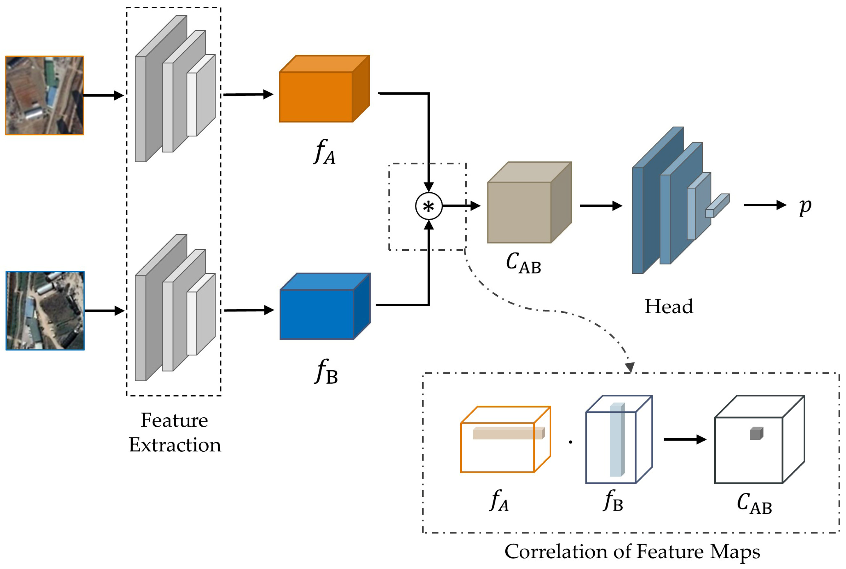
Remotesensing 13 03443 g001
Figure 2. Architecture of ScoreCNN. c A B = f A , f B represents the scalar product in C A B , where f A f A ,   f B f B .
Remotesensing 13 03443 g002
Figure 3. Architecture of ScoreCNN’s head. This part takes a correlation map as input and outputs the probability representing matching quality. Conv 3 × 3, 128 denotes a convolutional layer with a kernel of size 3 × 3 and the number of output channels 128.
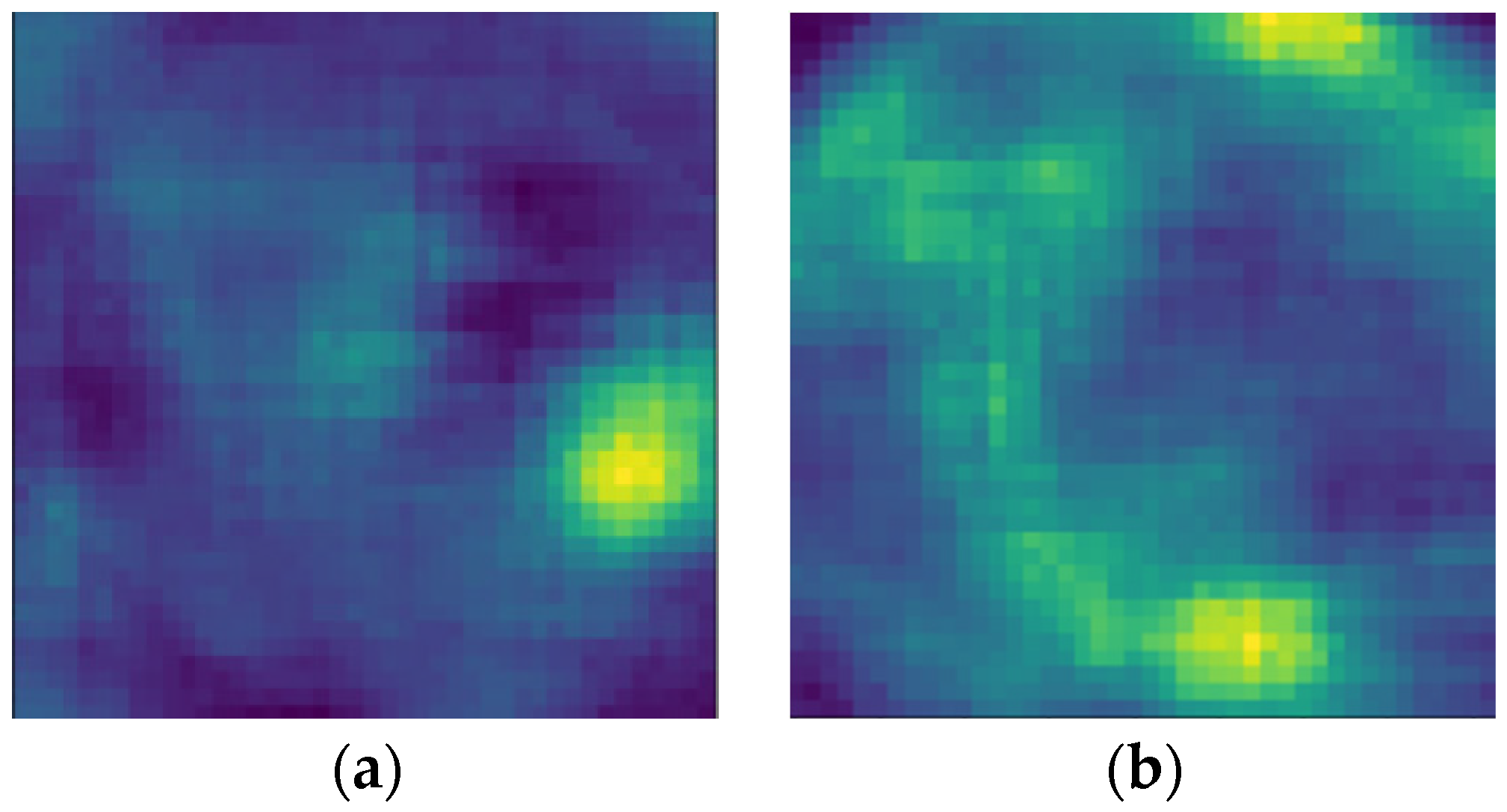
Remotesensing 13 03443 g003
Figure 4. Heatmaps M k generated with sliding windows. (a) is an ideal heatmap with a single peak; (b) is a heatmap with multiple peaks.
Remotesensing 13 03443 g004
Figure 5. Examples of sub-images pairs. (a) is a matched pair, (bd) are unmatched pairs.
Remotesensing 13 03443 g005
Figure 6. Network architecture of ETP. I s and I t represent the input source sub-images and the target sub-images, respectively. C 1 represents the correlation map from I s , 1 and I t , 1 . ( x s , y s ) and ( x t , y t ) represent the coordinates of the images to which they belong. v A and v B denote the 2-D vectors after encoding. v A , v B , and C are concatenated into feature block V . A θ denotes the final transformation matrix.
Remotesensing 13 03443 g006
Figure 7. Architecture of regression head. Inputs are the feature blocks V of the sub-image pairs. (a) is the basic architecture, (b) and (c) are the structure A and B respectively. Weight blocks generate the weight distribution α for V .
Remotesensing 13 03443 g007
Figure 8. Example of generating training samples. The orange boxes indicate the cropped sub-images from the source image, the orange dotted boxes indicate the location where the corresponding sub-images lie after transformation, the blue boxes indicate the cropped target sub-images, and the red boxes indicate the sub-images out of boundaries.
Remotesensing 13 03443 g008
Figure 9. Augmentation of positive training samples. Two conditions of the bounding rectangle in different sizes are shown. The orange boxes indicate the source sub-images after transformation, the blue boxes indicate the corresponding target sub-images and the grey boxes indicate the bounding rectangles of the orange boxes. The red points are the centers of the sub-images, and the black arrows show the scope where the windows of augmented target sub-images can randomly shift.
Remotesensing 13 03443 g009
Figure 10. The example of distribution of sub-images in the original images ( n s = 36), where “+” represents the centers of sub-images. (a) is the source image, (b) is the target image. The coordinates are normalized to [−1, 1], which shows that the distribution is not strictly grid aligned.
Remotesensing 13 03443 g010
Figure 11. Comparison of different architectures. (a) shows the trends of training loss and (b) shows the trends of MAE grid with the training process.
Remotesensing 13 03443 g011
Figure 12. Examples of the weight assignment to the sub-images. (ad) are the partial pairs in the same source image and target image, and (e) shows the comparison of the weights.
Remotesensing 13 03443 g012
Figure 13. AMR and AMP of at different n s .
Remotesensing 13 03443 g013
Figure 14. Comparison of qualitative registration results. Rows are pair 14 respectively. The alignment results are displayed in the form of checkerboard overlays. Significant local details are marked with red boxes and yellow boxes in the results of other methods and ours, respectively.
Remotesensing 13 03443 g014
Figure 15. Registration of a group of multi-temporal remote sensing images from other times and region. Rows are each as follows: (1) the source images, (24) overlays of the target image and the result warped by SIFT, DAM, and ours, respectively, (5) the identical target images taken in 2020.
Remotesensing 13 03443 g015
Figure 16. The registration results of images with massive changes.
Remotesensing 13 03443 g016
Figure 17. The registration results of images in ISPRS [51] (Row 1 and 2) and WHU [52] (Row 3).
Remotesensing 13 03443 g017
Figure 18. The results of registration on images with slight changes. (ae) are different image pairs from the testing dataset. Rows are the source images, the target images and warped results by our method from top to bottom. “o” and “x” denote the keypoints in the source images and target images, respectively.
Remotesensing 13 03443 g018
Figure 19. The failure case on the images with large resolution variance. The original resolution of the source image is 412 × 412, and 1260 × 1260 of the target image.
Remotesensing 13 03443 g019
Table 1. Comparison of different backbones of ScoreCNN. Acc represents the accuracy. F1 represents the harmonic average of precision and recall. FPR95 represents the false positive rate at the true positive rate of 95%. Param and FLOPs represent the number of parameters and floating-point operations of the models, respectively.
BackboneVGG-16ResNet-18
Acc88.8%88.6%
F10.880.88
AUC0.9600.957
FPR950.230.25
Param7.97 M3.11 M
FLOPs16.11 G1.66 G
Table 2. The layers in each block of regression head. Each row denotes a convolutional layer (size, kernels) with a default stride of 1 and padding of 0, followed by rectified linear units (ReLU).
BlockOutputSetting
Channel Attention15 × 1514-d fc,
227-d fc,
Conv05 × 5 [ 7 × 7 ,   128 5 × 5 ,   64   ] .
Template15 × 15 [ 3 × 3 ,   14 3 × 3 ,   227   ]
Wght1 × 1global average pool,
[ 1 × 1 ,   14 1 × 1 ,   1   ] ,
softmax,
Conv13 × 3 [ 3 × 3 ,   256 7 × 7 ,   128 5 × 5 ,   64 ]
FC1 × 1128-d fc,
6-d fc
Table 3. Percentage of images per category and per subset.
DatasetUrban LandscapesCountrysideVegetationWaters
Training37.3%34.0%20.5%8.2%
Validation45.6%30.0%14.9%9.5%
Testing34.9%34.7%26.3%6.1%
Table 4. The experimental parameter settings.
NotationParameterDefault Value
n s Number of cropped source sub-images36
T H Threshold of filtering weak-texture images0.3
r Radius of the neighborhood in Algorithm 15
t Difference between the first and second peak in Algorithm 11
l Lower limit of the maximum in Algorithm 10.5
m Minimum of sub-image pairs1
T s Threshold of similarity scores in ETP2
s t Interval of candidate sub-images in target images20
Table 5. Comparative results of different architectures and inference procedures on validation set. “S→T” and “T→S” indicate the predicted transformations in two inference directions of the same trained model. “Bidirection” refers to the two-stream model trained bidirectionally and as an ensemble.
ArchitectureGrid Loss   M A E g r i d
BasicS→T0.00914.87
BasicT→S0.00914.92
BasicBidirection0.03218.45
Struct. AS→T0.00513.13
Struct. AT→S0.00513.18
Struct. ABidirection0.01514.45
Struct. BS→T0.00411.59
Struct. BT→S0.00411.62
Struct. BBidirection0.01813.60
Table 6. Effects of the augmentation on ScoreCNN.
ModelAccuracyF1AUCFPR95
ScoreCNN (without Aug.)93.8%0.920.9820.085
ScoreCNN (with Aug.)94.5%0.930.9840.067
Table 7. Effects of the augmentation on ETP.
ModelGrid Loss   M A E g r i d
ETP (without Aug.)0.00512.35
ETP (with Aug.)0.00411.59
Table 8. Comparison of probability of correct keypoints (PCK) for registration with different methods on testing set. The whole registration stream for SIFT is SIFT + Random Sampling and Consensus (RANSAC) [48]. ‘Int. Aug.’ + ‘Bi-En.’ represents the best one in [45]. The scores marked with “†” were brought from [45] and evaluated on the same dataset. The models in the two-stage approach we proposed are in single-stream architecture, and n s denotes the number of cropped source sub-images.
MethodsPCK (%)
α = 0.05 α = 0.03 α = 0.01
SIFT [54]51.2 45.9 33.7
DAM (Int. Aug. + Bi-En.) [45]97.1 91.1 48.0
Two-Stage approach (Basic, n s = 25 )98.3 91.9 49.5
Two-Stage approach (Struct. A, n s = 25 )99.1 95.3 51.2
Two-Stage approach (Struct. B, n s = 25 )99.3 96.5 58.9
Two-Stage approach (Struct. B,   n s = 36 )99.297.464.8
Table 9. Comparison of quantitative results. Columns 1~4 represent the errors of registration for pair 1–4 in Figure 14 respectively. “\” represents the failure of registration. MAE: Mean absolute error.
MethodMAE (Pixels)
1234
SIFT\\122.43\
DAM (Int. Aug. + Bi-En.)18.7016.8056.9493.48
Two-Stage approach (Struct. B,   n s = 2 5)2.835.316.919.62
Table 10. Comparison of registration results on the images displayed in Figure 18.
MethodMAE (Pixels)
abcde
SIFT1.778.630.422.441.41
DAM (Int. Aug. + Bi-En.)8.5212.643.8312.852.53
Two-Stage approach (Struct. B,   n s = 2 5)2.782.982.392.812.11
Publisher’s Note: MDPI stays neutral with regard to jurisdictional claims in published maps and institutional affiliations.

