CCT: Conditional Co-Training for Truly Unsupervised Remote Sensing Image Segmentation in Coastal Areas

Abstract

As the fastest growing trend in big data analysis, deep learning technology has proven to be both an unprecedented breakthrough and a powerful tool in many fields, particularly for image segmentation tasks. Nevertheless, most achievements depend on high-quality pre-labeled training samples, which are labor-intensive and time-consuming. Furthermore, different from conventional natural images, coastal remote sensing ones generally carry far more complicated and considerable land cover information, making it difficult to produce pre-labeled references for supervised image segmentation. In our research, motivated by this observation, we take an in-depth investigation on the utilization of neural networks for unsupervised learning and propose a novel method, namely conditional co-training (CCT), specifically for truly unsupervised remote sensing image segmentation in coastal areas. In our idea, a multi-model framework consisting of two parallel data streams, which are superpixel-based over-segmentation and pixel-level semantic segmentation, is proposed to simultaneously perform the pixel-level classification. The former processes the input image into multiple over-segments, providing self-constrained guidance for model training. Meanwhile, with this guidance, the latter continuously processes the input image into multi-channel response maps until the model converges. Incentivized by multiple conditional constraints, our framework learns to extract high-level semantic knowledge and produce full-resolution segmentation maps without pre-labeled ground truths. Compared to the black-box solutions in conventional supervised learning manners, this method is of stronger explainability and transparency for its specific architecture and mechanism. The experimental results on two representative real-world coastal remote sensing datasets of image segmentation and the comparison with other state-of-the-art truly unsupervised methods validate the plausible performance and excellent efficiency of our proposed CCT.

1. Introduction

Image segmentation, one of the most fundamental and important research topics in remote sensing, mainly concerns the process of partitioning the image into multiple non-interesting regions, among which the pixels in each one belongs to an identical land cover category and the pixels in any two adjacent ones belong to diverse categories [1,2]. As an initial step of other relevant remote sensing image analysis tasks, it plays a vital role and draws considerable attention. In recent years, with the continuous development of Earth observation technology, an increasing number of remote sensing images have been more easily accessible. Due to their wide coverage and high resolution, current remote sensing images provide abundant detailed land cover information, making them highly valuable for a wide range of real applications, for example, road centerline extraction [3], building footprint extraction [4], land cover mapping [5], and change detection [6]; however, they suffer from more redundancy and noise. Therefore, remote sensing image segmentation is not only a profound task but also a challenging problem [7].

Over the past decade, the advent and development of deep learning technology have shown the fastest growing trend and proven to be both an unprecedented breakthrough and a powerful tool in many fields. Various classic neural network (NN) models, such as recurrent NN (RNN) [8], basic convolutional NN (CNN) [9], fully convolutional network (FCN) [10], generative adversarial network (GAN) [11], etc., have emerged and achieved remarkable performance in multiple image-processing tasks, including but not limited to image segmentation. Relying on the powerful capabilities in feature expression and data fitting, these models or their variations have been extensively applied in remote sensing, for example, scene classification [12], super-resolution [13], ice-wedge detection [14], and damaged building identification [15]. For remote sensing image segmentation, according to diverse algorithms, current deep learning-driven approaches can be broadly classified into three principal categories, which are fully supervised, semi-supervised, and transfer learning-based ones, respectively.

Fully supervised methods generally regard image segmentation as a specific type of one-sided pixel-level mapping task and attempt to simulate this process using an end-to-end model. Wang et al. [16] introduced a gated CNN for semantic segmentation of high-resolution images. Fu et al. [17] combined the strengths of FCNs and conditional random fields (CRFs) and proposed an accurate classification method for high resolution remote sensing imagery. Liu et al. [18] took advantage of several advances in CNN designs and proposed an hourglass-shaped network to segment aerial images. Diakogiannis et al. [19] integrated a UNet with the residual connection and developed a ResUNet-a network for semantic segmentation. Yang et al. [20] applied the attention mechanism and developed an attention-fused network for semantic segmentation. These methods are advantageous at the directness and simplicity of their working mechanisms, which can achieve the best performance, even competing with the human visual system. Nevertheless, nearly all the success depends on sufficient high-quality pre-labeled training samples, which are label-intensive and time-consuming. In addition, this type of enclosed black-box solution lacks explainability and transparency, which has always been criticized and questioned.

Semi-supervised methods substantially still follow the standard training protocol of fully supervised ones but require the assistance of some advanced strategies and human intervention. Zhang et al. [21] proposed a new framework, combining active learning and hierarchical segmentation, for spectral-spatial classification of hyperspectral images. Hua et al. [22] took incomplete annotations into account and achieved the feature and spatial relational regularization in the process of semantic segmentation. Niu et al. [23] adopted a generic CNN to iteratively modify the segmentation mask and performed aerial image segmentation. Wang et al. [24] integrated ideas of consistency regularization and an average update of pseudo-label and applied a teacher–student model for semantic segmentation. Protopapadakis et al. [25] employed four semi-supervised learning schemes and applied a stack autoencoder-driven CNN to extract buildings from near infrared images, with an extremely small portion of data. Compared to fully supervised methods, semi-supervised ones have improved the utilization of training samples and model interpretabilities, and meanwhile, they still perform well when facing the issue of unbalanced sample categories. However, if the domain discrepancy of training and testing samples is large enough, the well-trained models in both types of methods yield unsatisfactory performances.

Transfer learning-based methods thoroughly consider the problem of domain gaps and attempt to utilize a set of labeled training samples to achieve reference-free semantic segmentation of other datasets. Focusing on image domain mismatches, Zhang et al. [26] proposed a curriculum-style domain adaptation network for cross-domain segmentation. Zou et al. [27] proposed an unsupervised domain adaptation framework to eliminate the large discrepancy of the source and target data, which was guided by the class-balanced self-training strategy. Li et al. [28] developed a bidirectional model and a self-supervised learning algorithm to jointly realize domain adaptation and image segmentation. Luo et al. [29] integrated ideas of co-training and adversarial learning and proposed a category-level adversarial network to enforce local semantic consistency during the trend of global feature alignment. Fang et al. [30] embedded a geometry-consistent GAN in a co-training adversarial network and introduced a category-sensitive domain adaptation method for land cover mapping using optical aerial images. Although most classic transfer learning models are specifically designed for natural images, they can still be directly utilized for remote sensing ones. In practice, based on their specific mechanisms, these methods can effectively distill high-level semantic knowledge from remote sensing images. However, the structures of GAN-based models are generally quite complex, leading to low training efficiency and unstable convergence procedure.

Different from common natural images, coastal remote sensing ones generally carry more complicated and considerable land cover information [31,32]. In reality, it is mainly reflected in three aspects: (1) ground targets are susceptible to the environmental factors, such as imaging time, seasonal variation, and illumination intensity, as shown by the red circles in Figure 1, where the farmlands without crops have diverse texture distributions; (2) different categories of targets display low inter-class variances, as shown by the green box in Figure 1, where the paddy fields and water have similar appearances; (3) the same category of targets display high intra-class variances, as shown by the blue box in Figure 1, where the upland fields with different crops have diverse appearances. To address the above problems, in our previous research [33,34], we have proposed a fully supervised model and a transfer learning-based model for image segmentation using coastal remote sensing images. However, we find that, in addition to the primary land cover categories, including water, vegetation, buildings, roads, and impervious surfaces, certain particular coastal elements may be agnostic to any exact category [35]. All the observation indicates that it is difficult to manually pre-label the coastal remote sensing images specifically for image segmentation, even with advanced deep learning strategies [36,37]. Therefore, it is very essential to explore truly unsupervised image segmentation algorithms.

To relive the aforementioned limitations, in this paper we investigate the utilization of NNs for unsupervised learning, then propose a novel method, namely, conditional co-training (CCT), specifically for truly unsupervised remote sensing image segmentation in coastal areas. To drive our idea, a global image filter, a replaceable encoder, and two constant decoders are composed to a multi-model framework to simultaneously perform the pixel-level classification. This framework comprises two parallel data streams, which are superpixel-based over-segmentation and pixel-level semantic segmentation. They aim to separately process the input images into two different types of segmentation maps in the forward procedure. Nevertheless, in the backward procedure, the former iteratively fine-tunes the outputs of the latter and provides self-constrained guidance for model training, and the latter continuously outputs multi-channel response maps. By training our multi-model framework with multiple conditional constraints between these two data streams, our method progressively learns to perform reference-free image segmentation, which is of stronger explainability and transparency when compared to the black-box solutions in supervised learning manners. In summary, this work has the following contributions:

• We introduce a novel deep learning-driven approach for truly unsupervised remote sensing image segmentation in coastal areas. In this method, the advantages of both conventional and deep learning algorithms are seriously taken into consideration.
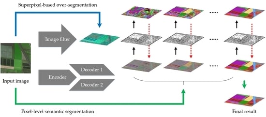
• We introduce a multi-model deep learning framework to drive our idea. To the best of our knowledge, this is the first time simultaneously applying ideas of superpixels and co-training in unsupervised image segmentation tasks.
• We adopt multiple conditional constraints, including pixel similarity, superpixel continuity, classification consistency, and decoder diversity, then specifically design a novel objective to facilitate training our framework.
• Considering the uncertainties in unsupervised learning, we perform comprehensive discussions on the settings and designs of our framework to explore the optimal determinations of the global image filter and deep learning model architectures.

The Section 1 is introduction. The remainder of this paper is arranged as follows. The background of our research is briefly introduced in Section 2. The methodology regarding formulation, objective, and implementation of our proposed CCT is elaborated in Section 3. The experimental results and their evaluations on two datasets are presented in Section 4. Relevant discussions on the settings and designs of our models are performed in Section 5. Finally, the conclusion of this research is summarized in Section 6.

2. Background

2.1. Superpixels

With the rapid development of Earth observation technology, the spatial resolution of remote sensing images has gradually improved, providing abundant image information but more noise and redundancy. In this case, the pixel-level features are seriously lacking representativeness, and regarding them as the elementary units in image understanding tasks leads to numerous errors. Recently, relevant researches have shifted to increasingly rely on superpixels, which group pixels into perceptually meaningful regions. Since they provide more convenient primitives from which to analyze images, and distinctly reduce the complexity of subsequent image analysis tasks, superpixel-based over-segmentation processes have become the key blocks of extensive computer vision algorithms. To better alleviate the negative influences from noise and redundancy, the superpixel-based image segmentation methods should strictly adhere to the following three protocols:

• The pixels with similar visual features should belong to the same superpixel.
• The contiguously distributed superpixels should be assigned as the same category.
• The scales of all superpixels should be larger than the size of the smallest object.

Although some of the above protocols are incompatible and may never satisfy each other perfectly, simultaneously considering all of them is still beneficial to produce the optimal results of image over-segmentation.

The concept of superpixels goes back at least to the image Gestalt theory [38], which developed various principles for perceptual grouping, such as proximity, similarity, and continuation. Thereafter, Vedaldi et al. [39] took superpixels as the image primitives and introduced an efficient clustering algorithm, which explicitly traded off under- and over-fragmentation. Levinshtein et al. [40] described a geometric-flow-based algorithm, which was very fast and could even be applied to megapixel-sized images with high superpixel densities. Veksler et al. [41] observed the irregularity of superpixels, then formulated the partitioning problem in an energy minimization framework, which was optimized using graph cuts. Numerous relevant reports suggest that superpixels are the most meaningful and optimal elementary units for image segmentation.

2.2. Co-Training

In practical, the capability volumes of current deep learning models are greater than the information content of images, leading to a high possibility of data overfitting during the training process. Unfortunately, merely simplifying the model structures may reduce their capabilities in feature expression, and then distinctly reduce the utilization of image information. To address this problem, the co-training strategy is established based on the theory that the solution in tasks, such as image segmentation and semantic labeling, is not unique. Different from the single chained models in general deep learning methods, this strategy is characterized by multi-view learning in which learners are trained alternately on two or more views from unlabeled data. Specifically, for image segmentation tasks, it is suggested to simultaneously train two classifiers on two single views, but for the same purpose. Along this way, the two classifiers and the corresponding outputs should meet the following three requirements:

• Both classifiers can perform well and produce similar outputs on the same dataset.
• Both classifiers are simultaneously trained on strictly different images.
• Both classifiers are likely to satisfy Balcan’s condition of $ϵ$-expandability [42], which is a necessary and sufficient pre-condition for co-training to work.

All the above principles substantially enforce the two classifiers to be always diverse but achieve the same performance, even without references [43]. The diversity between these two models is mainly reflected in their learned parameters, and currently there are many tricks that can be applied to reach this purpose, for example, dropout regularization [44], consensus regularization [45], and parameter diverse [46].

The co-training strategy was first introduced for data combination [47], which used large unlabeled samples to boost the performance of a learning algorithm when only a small set of labeled examples was available. Thereafter, Chen et al. [48] introduced a variant of co-training and applied it in domain adaptation. To further improve the learning ability, Saito et al. [49] proposed an asymmetric tri-training algorithm, which kept two classifiers producing pseudo labels and then used them to train a third classifier. As a considerable innovation in the development from supervised to unsupervised learning, this algorithm is practically appropriate and essential for unsupervised image segmentation.

3. Methodology

In this section, the problem formulation of unsupervised image segmentation using coastal remote sensing images is first presented. Secondly, the full objective of our multi-model framework is defined and interpreted in detail. Finally, relevant implementations regarding the network architectures and training details are described.

3.1. Formulation

Given a remote sensing image $I$ that is captured in coastal areas, the main goal is to learn a framework that can effectively extract semantic features from it and precisely perform pixel-level classification for it. As described by Kanezaki et al. [50], the input image can be regarded as a finite collection of pixels ${\left\{P_n\in {ℝ}^3\right\}}_{n=1}^N$, where $P$ and $N$ denote the pixel value and the total number of pixels, respectively. In the case of pre-labeled classification maps ${\left\{C_n\in \mathbb{Z}\right\}}_{n=1}^N$, where $C$ denotes the category to which each pixel belongs, the segmentation model can be regarded as a mapping function $G:{ℝ}^3\to \mathbb{Z}$, which is trained in a supervised learning manner. Along this way, all the pixels are transferred from their original matrix space to the category space by $\left\{C_n\right\}=G\left(\left\{P_n\right\}\right)$. However, in this research, the category attributes and the total number of categories are both completely unknown, say in a nutshell, there is no ground truth to facilitate training the model in a supervised learning manner. In this situation, two important sub-problems are essential to be settled urgently, which are the optimal prediction of $\left\{C_n\right\}$ and the parameter training of $G$. Although the definition of categories is independent of the segmentation model, there must be some mutually restrictive relationships between them. Motivated by this observation, we adopt the concept of superpixels and introduce a multi-model framework to simulate the process of our proposed CCT, as illustrated in Figure 2. This framework is composed of two parallel data streams, namely, superpixel-based over-segmentation and pixel-level semantic segmentation. They are structurally independent and will not interact with each other in the forward propagation, while the former will constantly guide the latter in the backward propagation, aiming to facilitate training all the models.

As the driving draft of our method, the superpixel-based over-segmentation stream aims to divide the input image into excessive segments in which all of the pixels have similar feature distributions. Achieved by a global superpixel-based image filter $F$, the process of this stream is formulated as shown in Equation (1).

$$I_S=F\left(I\right)$$

(1)

where $I_S$ is the over-segmentation map that can be regarded as the regional distribution of superpixels ${\left\{S_k\in {ℝ}^1\right\}}_{k=1}^K$, where $S$ and $K$ denote the superpixel region and the total number of superpixels, respectively. Specific to the superpixel-level, this process can also be formulated as shown in Equation (2).

$$\left\{S_k\right\}=F\left(\left\{P_n\right\}\right)$$

(2)

where $K$ is less than $N$, but much larger than the total number of land cover categories. In addition, the size of each superpixel should not be less than that of the smallest meaningful object on the image, making all of the possible inter-class contours are completely outlined by the superpixel boundaries. Therefore, the total number of superpixels can be initially set as shown in Equation (3).

$$K=\frac{W\times H}{{\delta }^2\cdot {\mathcal{O}}_{min}}$$

(3)

where $W$ and $H$ are the width and height of an input image, respectively. $\delta$ means the image scale and ${\mathcal{O}}_{min}$ denotes the size of the smallest meaningful ground target, such as cars or isolated buildings.

As the driven draft of our method, the pixel-level semantic segmentation stream has the analogous mechanism as an end-to-end deep learning model, which aims to translate the input image to a response map based on pseudo categories. Simultaneously achieved by one replaceable encoder $En$ and two constant decoders $\left\{D{e}_1,D{e}_2\right\}$, the process of this stream is formulated as shown in Equation (4).

$$I_R=I_R^{\left(1\right)}+I_R^{\left(2\right)}=D{e}_1\left(En\left(I\right)\right)+D{e}_2\left(En\left(I\right)\right)$$

(4)

where $I_R$ is the response map that can be recognized as the probabilistic distribution of pseudo categories ${\left\{R_n\in {ℝ}^M\right\}}_{n=1}^N$, where $R$ and $M$ denote the pixel pseudo category and the total number of pseudo categories, respectively. $I_R^{\left(1\right)}$ and $I_R^{\left(2\right)}$ denote two secondary response maps, which are produced by those two decoders.

With these two data streams, the training and testing processes simultaneously take place. In the forward propagation, as the latter stream outputs a multi-channel category-based response map, the former stream will fine-tune it with the assistance of $\left\{S_k\right\}$, then produces a refined response map, which can also be recognized as a periodical reference segmentation map. In the backward propagation, the three deep learning models will be alternately updated under the guidance of a refined response map, similar to supervised learning manners. Here, the refinement is defined as shown in Equation (5).

$$R_n^{*}=\mathrm{count}\max \left\{R_{n_1},R_{n_2},\dots ,R_{n_t}\right\}n\in \left\{n_1,n_2,\dots ,n_t\right\}\in S_k$$

(5)

where $n_t$ denotes the $t$th pixel that belongs to $S_k$. In addition, particularly for the latter stream, there are two more conditions that need to be taken into account. The first one is that the outputs of two decoders should be similar at the pixel level, which is defined as shown in Equation (6). The second one is that the weights of two decoders should be diverse, which is defined as shown in Equation (7).

$$I_R^{\left(1\right)}\left(i,j\right)\approx I_R^{\left(2\right)}\left(i,j\right)$$

(6)

$$\overrightarrow{D{e}_1}\perp \overrightarrow{D{e}_2}$$

(7)

where $I_R\left(i,j\right)$ means the response value of the pixel located at $\left(i,j\right)$, and $\to$ denotes the one-dimensional vector representation of all weights in a model. Analogous to the above refinement, these two conditions will alternately facilitate updating the three deep learning models in the backward propagation.

With the iterative optimization of this multi-model framework, the total number of pseudo categories continues to decline, and meanwhile, the response map progressively approaches the probability distribution of real land cover categories. Along this way, the final predicted pixel-level classification map can be obtained by a basic argmax function, which is expressed as shown in Equation (8).

$$C_n^{*}=\arg \max \left\{R_n^{\left(1\right)},R_n^{\left(2\right)},\dots ,R_n^{\left(M\right)}\right\}$$

(8)

3.2. Objective

With our multi-model framework, several important constraints, including the pixel similarity, superpixel continuity, category consistency, and decoder diversity, are highly emphasized and seriously considered. Meanwhile, based on these constraints, we design four corresponding loss functions, and then introduce a novel objective for unsupervised remote sensing image segmentation in coastal areas. In the following, each component of this objective is described and interpreted in detail.

3.2.1. Pixel Similarity

In general, most deep learning-driven semantic segmentation models end up with a fully connected layer, which aligns the multi-channel response map to the single-channel pre-labeled reference using a SoftMax-like loss. In this work, although there is no ground truth to supervise the training of models, the pixel similarity can still be recognized as an important basis specifically for image segmentation, which provides self-supervision for the automatic pixel clustering. Derived from Kanezaki et al. [50], an argmax classification strategy is adopted as our segmentation principle. Intuitively, the predicted category $C_n$ for each pixel is mainly obtained by selecting the dimension that has the maximum value in the corresponding response map $R_n$ no matter what specific category it belongs to, as illustrated in Equation (8). To implement this condition, we design the constraint of pixel similarity to assign all pixels of similar visual features to the same category, even though some pixels are distant from others on the original image. Along this way, this constraint can be quantified as a cross entropy loss between $\left\{C_n\right\}$ and $\left\{R_n\right\}$, which is formulated as shown in Equation (9).

$${ℒ}_{PS}={\displaystyle \sum }_{n=1}^N{\displaystyle \sum }_{m=1}^M-\phi \left(C_n,m\right)\cdot \log R_n^{\left(m\right)}$$

(9)

where $\phi \left(C_n,m\right)$ denotes a conditional operation, as defined in Equation (10).

$$\phi \left(C_n,m\right)=\{\begin{array}{c}1 if C_n=m\\ 0 if C_n\ne m\end{array}$$

(10)

Minimizing this loss will enforce the feature distributions of pixels in the same predicted category to be similar to each other, then facilitate our encoder to efficiently extract more meaningful high-level features for unsupervised clustering.

3.2.2. Superpixel Continuity

For a well over-segmentation map, the pixels in the same superpixel display similar appearances, and they are more likely to belong to the same pseudo category. Therefore, in the corresponding response map, each superpixel should be continuous for its feature distributions. Considered by Kim et al. [51], it is preferable for the clusters of pixels to be spatially continuous and exploring an additional constraint on the relationship between the cluster labels and their neighboring ones is very essential. Relevant reports generally concentrate only on the global continuity and ignore the importance of a local one, leaving some regions of the segmentation map with numerous ambiguous predictions. To avoid this situation, we adopt the constraint of superpixel continuity to ensure each superpixel to be consistent in the feature distribution. Concretized from Equation (5), this constraint can be quantified as a loss function, which is formulated as shown in Equation (11).

$${ℒ}_{SC}={\displaystyle \sum }_{k=1}^K{\displaystyle \sum }_{t=1}^T\Vert R_{n_t}-R_n^{*}{\Vert }_2 n\in \left\{n_1,n_2,\dots ,n_t\right\}\in S_k$$

(11)

where ${\Vert \cdot \Vert }_2$ is the L2 distance loss. Minimizing this loss will suppress the error predicted pixel-level categories caused by complicated patterns or textures, then distinctly enhance our two decoders’ resistance to image noise and redundancy.

3.2.3. Category Consistency

Due to its specific mechanism, the co-training strategy is practically integrated with other deep learning techniques for unsupervised domain adaptation of semantic labeling tasks, and the corresponding loss function is generally embedded in other full objectives. From our perspective, although this strategy is not strong enough as existing end-to-end mapping ones in supervised learning, it still provides a rigorous constraint if added with certain reliable conditions in either supervised or unsupervised learning. As observed by Fang et al. [29], the same prediction of a pixel by two classifiers offers high confidence in its classification result, even without references. Motivated by this observation, we adopt the constraint of category consistency to make our two decoders supervise each other for their alternate updating. Concretized from Equation (6), this constraint can be quantified as a loss function, which is formulated as shown in Equation (12).

$${ℒ}_{CC}={\displaystyle \sum }_{i=1}^W{\displaystyle \sum }_{j=1}^H\Vert I_R^{\left(1\right)}\left(i,j\right)-I_R^{\left(2\right)}{\left(i,j\right)\Vert }_1$$

(12)

where ${\Vert \cdot \Vert }_1$ is the L1 distance loss. Alternatively, this constraint can also be quantified in a type of weaker form, which is formulated as shown in Equation (13).

$${ℒ}_{CC}={\displaystyle \sum }_{i=1}^W{\displaystyle \sum }_{j=1}^{H}1-\cos \left(I_R^{\left(1\right)}\left(i,j\right),I_R^{\left(2\right)}\left(i,j\right)\right)$$

(13)

Minimizing this loss will make our two decoders output similar multi-channel category-based response maps, then significantly increase the stability of our framework in image segmentation tasks.

3.2.4. Decoder Diversity

As described by Zhou et al. [52], the classifiers in co-training should always be kept diverse, otherwise all the semantic segmentation maps predicted by them will be exactly the same, making co-training degenerate to self-training with a single classifier. In effect, early researches usually use sufficient and redundant views to enable these classifiers be different, which strictly follows the standard co-training principle. Nevertheless, current extended researches choose to directly set certain conditions to reach this purpose. Based on this mechanism, we adopt the constraint of decoder diversity to enforce divergence of the weights of convolutional layers in our two decoders by minimizing their cosine similarity. Concretized from Equation (7), this constraint can be quantified as a loss function, which is formulated as shown in Equation (14).

$${ℒ}_{DD}=\frac{\mathcal{W}\left(D{e}_1\right)\cdot \mathcal{W}\left(D{e}_2\right)}{\Vert \mathcal{W}\left(D{e}_1\right)\Vert \cdot \Vert \mathcal{W}\left(D{e}_2\right)\Vert }$$

(14)

where $\mathcal{W}(\cdot )$ denotes the operation that collects all the weights of a network, then flatten and stack them into a one-dimensional vector. $\Vert \cdot \Vert$ means the norm of a vector. Minimizing this loss will make our two decoders orthogonal vectorially, then effectively improve the generalization of our framework in image segmentation tasks.

In general, the full objective of our CCT is an integration of the aforementioned four constraints, which is formulated as shown in Equation (15). Therefore, the main solution for this full objective can be expressed as shown in Equation (16).

$$ℒ\left(En,D{e}_1,D{e}_2\right)={\lambda }_{PS}\cdot {ℒ}_{PS}+{\lambda }_{SC}\cdot {ℒ}_{SC}+{\lambda }_{CC}\cdot {ℒ}_{CC}+{\lambda }_{DD}\cdot {ℒ}_{DD}$$

(15)

$$E{n}^{*},D{e}_1^{*},D{e}_2^{*}=\arg \underset{En,D{e}_1,D{e}_2}{\min }ℒ\left(En,D{e}_1,D{e}_2\right)$$

(16)

where $\lambda$ denotes the relative importance of each constraint. Different from conventional supervised deep learning models, the training and testing of the multi-model framework are carried out on the same timeline and end up simultaneously. Thus, it is not necessary to specifically prepare the training and testing samples for our CCT. Accordingly, all the well-trained models are practically invalid for the untrained samples.

3.3. Implementation

3.3.1. Network Architectures

Our proposed CCT is mainly driven by a multi-model framework consisting of four models, which are a global superpixel-based image filter, a replaceable encoder, and two constant decoders, respectively. Only the latter three models are deep learning networks and the suggested architectures of them are illustrated in Figure 3. Derived from ResNet [53], the encoder comprises three convolutional blocks and six residual ones. This model conducts two-fold down-sampling on the input images, aiming to produce the high-level semantic features and pass them to the decoders. Inspired by Encoder-Decoder [54], each decoder comprises a transposed convolutional block and a convolutional block, followed by a single convolutional layer and a single normalization layer. These two models conduct two-fold up-sampling on the input feature maps, aiming to simultaneously produce the response map through element-wise summation of the two secondary ones. For these three models, all the parameters of their layers are initialized using the strategy of Xavier [55]. In addition, it is mentioned that our encoder is a replaceable deep learning network, which can refer to the down-sampling parts of any well-known model architecture, such as ResNet or VGG [56]. In this work, we highly recommend referring to ResNet because of its low model complexity and high training efficiency. Technically speaking, no matter what architecture is adopted in this encoder, using the corresponding pre-trained model as the initial one can significantly improve the convergence efficiency of the entire multi-model framework.

3.3.2. Training Details

For all the experiments, our primary goal is to learn well-trained models during the training process that minimizes the full objective $ℒ\left(En,D{e}_1,D{e}_2\right)$. In this work, according to the interpretation in BackProp [50], we apply SLIC [57] in our global superpixel-based image filter and set the compactness and max iteration of $F$ to 1 and 10, respectively, in Equations (1) and (2). Moreover, referring to the implementations in DFC [51] and CsDA [30], we set both ${\lambda }_{PS}$ and ${\lambda }_{SC}$ to 1, and set ${\lambda }_{CC}$ and ${\lambda }_{DD}$ to 0.01 and 0.1, respectively, in Equation (15). To pursue the most optimal framework, we repeat the training process for multiple times, and finally choose the one with the best performance.

Given the complexity of our multi-model framework, the alternate learning strategy is utilized to accelerate the convergence of all models. In each iteration, the input remote sensing image is forwarded into our three deep learning models for one time. Thereafter, the encoder is updated two times while the decoders are updated three times. The pseudo code and more details about our training process are presented in

Table 1. Overview of the training process for our multi-model framework.

Input:	Remote sensing image: $I=\left\{P_n\in {ℝ}^3\right\}$
$I\to F\Rightarrow I_S$ for$iteration\leftarrow 1 to iteratio{n}_{max}$do  forward: $I\to En,D{e}_1,D{e}_2\Rightarrow I_R\to I_S\Rightarrow \left\{R_n^{*}\right\}$  backward 1: update $En,D{e}_1,D{e}_2$ with ${ℒ}_{PS},{ℒ}_{SC},\left\{R_n^{*}\right\}$  backward 2: update $En,D{e}_1,D{e}_2$ with ${ℒ}_{CC}$  backward 3: update $D{e}_1,D{e}_2$ with ${ℒ}_{DD}$ end for $I_R\Rightarrow \left\{C_n^{*}\right\}$
Outputs:	Well-trained encoder: $E{n}^{*}$ Well-trained decoders: $D{e}_1^{*}$ and $D{e}_2^{*}$ Image segmentation result: $\left\{C_n^{*}\right\}$

.

4. Experiments

In this section, the datasets description, baseline methods, and evaluation metrics of this research are first introduced in detail. Thereafter, the experimental setup of our CCT is provided and interpreted. Finally, the experimental results and related analyses of our method and other comparative ones are presented.

4.1. Datasets Description

Provided by Chen et al. [34], two coastal remote sensing datasets are selected as the study areas in this research. The first dataset is located in the southeast of Shanghai City, China and was captured in 2016, while the second dataset is located in the northeast of Zhejiang Province, China and was captured in 2017. Obtained by Google Earth (DigitalGlobe), these two large-scale remote sensing images are located near the east coastline of China, each of which comprises three bands corresponding to the red (R), green (G), and blue (B) bands. As illustrated in Figure 4, the image in the Shanghai dataset covers approximately 46 square kilometers with the size of $11776\times 6144$, while the image in the Zhejiang dataset covers approximately 61 square kilometers with the size of $12800\times 7424$. However, the two images have the same spatial resolution, which is about 0.8 meters per pixel.

As can be seen, although both datasets are captured from the coastal areas of China, the appearances of them are distinctly diverse, which are principally caused by different imaging sensors, capture times, and illumination and atmospheric conditions. Moreover, influenced by the humid subtropical monsoon climate, some of the land cover categories display complex detailed features and low inter-class discrepancies, for example, vegetation, farmland, and water. Nevertheless, except for certain impervious surfaces and bare lands, most land cover categories display high intra-class similarities. In addition, all the land cover categories in the two datasets are proportionally unbalanced in terms of their coverage area. Generally speaking, the image in Shanghai dataset provides more detailed land cover information but more image noise and redundancy as compared with the one in Zhejiang dataset.

4.2. Baseline Methods

In this research, our proposed CCT is compared with other state-of-the-art unsupervised image segmentation methods. As the representatives of conventional ones, the two strategies, namely, the globalized probability of boundary (gPb) [58] and the ultrametric contour map (UCM) [59], respectively, are the best ones before 2010. The former one concentrates on the image contours and junctions and then develops a novel contour detector using a combination of local and global cues, offering a solid foundation for image segmentation tasks. The latter one adopts gPb as the backbone and then introduces a generic grouping algorithm that constructs a hierarchy of regions from the output of any contour detector, achieving region-based image segmentation. On the other hand, as the representatives of deep learning-driven ones, BackProp [50] and DFC [51] are the pioneers in exploring the utilization of CNNs for unsupervised image segmentation. Following the proposed three criteria, the former one chooses to train a simple NN only by backpropagation, while the latter one chooses to train it based on differentiable feature clustering. For the above five competitors, we perform all the experiments in unsupervised learning manners.

4.3. Evaluation Metrics

To validate the effectiveness and robustness of all comparative unsupervised image segmentation methods, three commonly used indicators are applied to comprehensively evaluate the corresponding experimental results, which are interpreted as follows.

Overall Accuracy (OA): this index is generally used to assess the total performance of the image segmentation methods, as expressed in Equation (17).

$$OA=\frac{1}{C}{\displaystyle \sum }_{c=1}^C\frac{T{P}_c+T{N}_c}{T{P}_c+T{N}_c+F{P}_c+F{N}_c}$$

(17)

where $T{P}_c$, $T{N}_c$, $F{P}_c$, and $F{N}_c$ indicate the numbers of true positive, true negative, false positive, and false negative pixels, respectively, for the $c$th land cover category.

Mean F1 Score (mF1): as the harmonic average of the precision and recall rates, this index is generally used to evaluate the NNs, as expressed in Equation (18).

$$mF1=\frac{1}{C}{\displaystyle \sum }_{c=1}^C\frac{2T{P}_c}{2T{P}_c+F{P}_c+F{N}_c}$$

(18)

Mean Intersection over Union (mIoU): by calculating the average of the ratios of the intersection and union for all categories, this index is regarded as a standard measure for classification-based methods, as expressed in Equation (19).

$$mIoU=\frac{1}{C}{\displaystyle \sum }_{c=1}^C\frac{T{P}_c}{T{P}_c+F{P}_c+F{N}_c}$$

(19)

Different from supervised image segmentation methods, unsupervised ones cannot directly produce the semantic segmentation maps. Relevant researches generally choose to align the segmented regions and the specified categories with the assistance of manual scribbles [60]. Based on this, the unsupervised methods can also be assessed normally. In addition, for the above three indicators, larger values suggest better results.

4.4. Experimental Setup

Different from supervised image segmentation methods, there is no need to initially prepare the non-overlapping training and testing samples for our CCT. Say in a nutshell, any region in the two datasets can be taken as an image sample, which will be input into our framework for simultaneously training and predicting. The only question that needs considered is how to select the size of input images. In theory, if the computing power of GPUs is powerful enough, the size of input images can be set to infinity. Nevertheless, in terms of the computing power of current common computers, we set the size of image samples to $512\times 512$. In addition, to accelerate the convergence of all parameters in the comparative deep learning models, we conduct mean subtraction normalization on each channel of image samples, from 0 to 255 to 0 to 1, before the experiments.

For the optimization process, we set two different termination conditions to achieve overall convergence, which are the maximum iteration number and minimum clustering number, respectively. In the training process, if the iteration number increases to ${10}^3$ or the clustering number decreases to 6, it is believed that the framework has converged. In addition, for the three deep learning models, we utilize stochastic gradient descent (SGD) with a momentum [61] of 0.9 as the optimizer, and the learning rate is initially set to 0.01 and progressively decayed to 0 by a poly learning rate policy.

In this research, our proposed CCT is implemented in PyTorch [62], which provides a high-performance environment with easy access to the automatic differentiation of models executed on different devices. All the experiments are performed on two computers with Intel Core i7, 32 GB RAM, and NVIDIA GTX 1080 GPU.

4.5. Training Visualization

In the training process, with our multi-model framework, certain representative images, their periodical segmentation results, and the corresponding convergence processes are presented in Figure 5. In general, the image segmentation of the Zhejiang dataset is basically completed at approximately the 150th iteration, which is visually faster than that of the Shanghai dataset.

With the convergence of our framework, the image segments progressively become complete, and meanwhile, their contours gradually become precise and smooth. Some of the large-scale ground targets, such as water and farmlands without crops, are accurately segmented and labeled the identical color, as shown in the second, third, and fourth columns in Figure 5. Nevertheless, certain upland fields are incorrectly labeled the different colors, as shown in the fifth and sixth columns in Figure 5.

4.6. Result Presentation

Based on the aforementioned two coastal datasets, the unsupervised remote sensing image segmentation results obtained by our CCT and other competitors are illustrated in Figure 6 and Figure 7, where the pixels in the same colors indicate that they belong to the same land cover categories. In general, the image segmentation results on the Zhejiang dataset are slightly better than those on the Shanghai dataset, because the land cover information on the latter one is more complex and diverse than that on the former one.

As shown in Figure 6a,b and Figure 7a,b, although the two conventional approaches perform well on small-scale natural images, they give unsatisfactory results on the large-scale coastal remote sensing images. Since gPb and UCM merely apply simple filters and linear statistics to analyze the pixels and their surroundings, they pay too much attention to the local details. This makes the results involve too many tiny segments, including the target contours, disrupted textures, and dense noises, which are completely meaningless for pixel-level semantic segmentation. Due to the limited capability in feature expression and global perceptron, gPb generally fails to detect the long-range spatial relations of the pixels that belong to the same categories. By contrast, UCM sorts the close local pixels by similarity and iteratively merges some similar regions, displaying a slightly better result. Nevertheless, for some large-scale targets, both methods still divide them into numerous different land cover categories, as depicted in the seventh row in Figure 6 and the fourth row in Figure 7. In general, conventional methods cannot extract the high-level semantic features, making them suitable for edge detection rather than image segmentation.

As shown in Figure 6c,d,e, and Figure 7c,d,e, deep learning-driven approaches yield significantly better performance than conventional ones, though there are still some gaps between their results and land cover ground truths. Relying on the powerful capabilities in feature expression and data fitting, deep learning models are able to effectively extract high-level semantic features and facilitate clustering the similar pixels, even though they are distant from each other. With the optimization of weight parameters, DFC displays a slightly better result than BackProp, specifically for targets with complicated textures. By integrating ideas of superpixels and co-training, our CCT can display better results than other competitors, which can not only produce the clear and complete regions of targets, but also alleviate the negative influences of image noise and redundancy. For large-scale regions, although our CCT fails to cluster all the pixels into the same category, it can still classify them into several sub-categories in terms of their target attributes, as depicted in the eighth row in Figure 6e and the fifth row in Figure 7e. It is confirmed that our CCT is effective and robust for unsupervised image segmentation tasks. In general, if with some assistances of input scribbles, the results of deep learning-driven methods can be further processed very close to the semantic segmentation references.

With the image segmentation results of all competitors and the corresponding input scribbles, the evaluation metrics OA, mF1, mIoU, and the processing rate on two datasets are calculated and summarized in

Table 2. Quantitative results of the comparative methods on Shanghai dataset. The best values are in bold.

Method	OA (%)	mF1 (%)	mIoU (%)	Rate (s/image)
gPb	40.47	29.32	21.43	23.60
UCM	41.75	31.03	22.92	89.25
BackProp	48.94	39.79	31.15	0.41
DFC	50.24	41.46	32.07	0.55
CCT	54.87	47.02	36.96	0.76

and

Table 3. Quantitative results of the comparative methods on Zhejiang dataset. The best values are in bold.

Method	OA (%)	mF1 (%)	mIoU (%)	Rate (s/image)
gPb	41.27	30.68	22.35	23.60
UCM	43.22	33.51	24.67	89.25
BackProp	53.30	45.83	35.39	0.41
DFC	55.61	49.17	37.82	0.55
CCT	58.49	52.24	41.10	0.76

. Compared to other state-of-the-art unsupervised methods, our proposed CCT achieves the highest OA, mF1, and mIoU on the two datasets. In addition, although our CCT is not the best in terms of processing rate, its training efficiency is definitely higher than all the supervised methods.

5. Discussion

For our proposed CCT, the final experimental performance is primarily determined by two decisive factors, which are the image filter and the model architecture. In this section, relevant discussions on our settings and designs of these factors are performed.

5.1. Setting of Image Filter

As the key guidance of our encoder and decoders, the over-segmentation results by the global superpixel-based image filter directly determine the qualities of unsupervised image segmentation. High-density over-segmentation maps record more precise contour information, which is beneficial to the separation of different categories. However, some of the large-scale regions are divided into too many tiny pieces, among which some may be meaningless for pixel-level classification, making the image segmentation results full of noises. In contrast, low-density over-segmentation maps display more meaningful segments, which have smooth boundaries and clear clustering centers. However, certain isolated small-scale objects may be grouped into the adjacent other categories, leading to some inevitable errors in the image segmentation results. Therefore, the proper setting of image filter is essential for better experimental performance. To pursue the most optimal setting of our global superpixel-based image filter, we kept the other models constant and conducted several comparative experiments with different settings of compactness and superpixel number in SLIC, and the results are presented in Figure 8 and Figure 9.

From the perspective of compactness, the lower value of it enforces superpixel contours to be smoother, making the segmented regions accurate and complete. However, certain false superpixel boundaries provide wrong guidance to the deep learning models, which may recognize part of a large-scale target as the other categories, as illustrated in the first column in Figure 8 and Figure 9. In contrast, higher value of it encourages superpixel contours to be squarer, making the segmented regions stable. However, the corresponding results are severely rasterized; furthermore, nearly all the region boundaries are heavily jagged, which distinctly contradicts the real information on the input images, as illustrated in the third column in Figure 8 and Figure 9.

From the perspective of superpixel number, the value of it determines the degree of over-segmentation. With a lower superpixel number, the average area of over-segments is larger, which can facilitate the deep learning models to learn implicit high-level features. However, the constraint of superpixel continuity will be indirectly reinforced, then some close pixels may be grouped into the same category, even if they have completely different appearances, as illustrated in Figure 8a and Figure 9a. In contrast, with a higher superpixel number, the average area of over-segments is smaller, which can effectively improve the classification capabilities of deep learning models. However, owing to the weakening on the constraint of superpixel continuity, the corresponding results may be plagued by the negative influences of noise and redundancy, as illustrated in Figure 8c and Figure 9c.

5.2. Design of Model Architecture

For different image-processing tasks, deep learning models are specifically designed with diverse architectures, aiming to pursue the best performance. Networks with larger depth and more complex structures generally have stronger capability in knowledge distillation, but they tend to overlook massive, detailed information on the input images. On the contrary, networks with smaller depth and simpler structures usually display higher training efficiency and stability, but their limited information capacities seriously hinder them from performing complicated classification tasks. Therefore, the optimal designs of our model architectures are important for better experimental performance. To pursue the most optimal designs of our encoder and decoders, we kept the image filter invariant and conducted several comparative experiments with different model architectures, where the numbers of down- and up-sampling operations are different, and the results are presented in Figure 10.

It is noteworthy that the models without any operation are sensitive to the detailed information and can always give the precise position and shape of each target; however, they are also suffering from the negative influences of noise and redundancy, as depicted in Figure 10a. As the operation number increases to three, the image segmentation results become more abstract, where nearly all the similar pixels and regions have been grouped into the same category, however, there are a wealth of deformations and distortions that appear in the results, as depicted in Figure 10c. In addition, for our three NNs, the less the operation number, the more parameters involved in updating, and the lower the training efficiency. Conversely, the more the operation number, the fewer parameters involved in updating, and the higher the training efficiency.

6. Conclusions

In this paper, we investigated the utilization of NNs for unsupervised learning and proposed a novel method, namely, CCT, for unsupervised remote sensing image segmentation in coastal areas. With the introduced multi-model framework and four conditional constraints, we successfully extracted high-level semantic knowledge and produced full-resolution segmentation results. The experiments on two coastal remote sensing datasets validated the plausible performance and excellent efficiency of our CCT, as compared to other state-of-the-art unsupervised image segmentation methods.

Nevertheless, our proposed method still involves a primary limitation. Without pre-labeled references, all of the conditional constraints are auto-correlative, which makes our framework sensitive to the over-segmentation maps. In each training process, our image filter may output a slightly different superpixel map where this tiny discrepancy will be continuously amplified by the deep learning models, leading to a visible diversity on the final image segmentation result, just like the butterfly effect. Therefore, in future studies, we plan to explore certain constants and robust constraints specifically for our framework to reduce the randomness of final image segmentation results.

References

1. Kotaridis, I.; Lazaridou, M. Remote Sensing Image Segmentation Advances: A Meta-Analysis. ISPRS J. Photogramm. Remote Sens. 2021, 173, 309–322. [Google Scholar] [CrossRef]
2. Yuan, X.; Shi, J.; Gu, L. A Review of Deep Learning Methods for Semantic Segmentation of Remote Sensing Imagery. Expert Syst. Appl. 2021, 169, 114417. [Google Scholar] [CrossRef]
3. Liu, R.; Song, J.; Miao, Q.; Xu, P.; Xue, Q. Road Centerlines Extraction from High Resolution Images Based on An Improved Directional Segmentation and Road Probability. Neurocomputing 2016, 212, 88–95. [Google Scholar] [CrossRef]
4. Xia, L.; Zhang, J.; Zhang, X.; Yang, H.; Xu, M. Precise Extraction of Buildings from High-Resolution Remote-Sensing Images Based on Semantic Edges and Segmentation. Remote Sens. 2021, 13, 3083. [Google Scholar] [CrossRef]
5. Mongus, D.; Zalik, B. Segmentation Schema for Enhancing Land Cover Identification: A Case Study Using Sentinel 2 Data. Int. J. Appl. Earth Observ. Geoinf. 2018, 66, 56–68. [Google Scholar] [CrossRef]
6. Zhang, X.; Xiao, P.; Feng, X.; Yuan, M. Separate Segmentation of Multi-Temporal High-Resolution Remote Sensing Images for Object-Based Change Detection in Urban Area. Remote Sens. Environ. 2017, 201, 243–255. [Google Scholar] [CrossRef]
7. Dey, V.; Zhang, Y.; Zhong, M. A Review on Image Segmentation Techniques with Remote Sensing Perspective. In Proceedings of the ISPRS TC VII Symposium—100 Years ISPRS, Vienna, Austria, 5–7 July 2010; pp. 31–42. [Google Scholar]
8. Hochreiter, S.; Schmidhuber, J. Long Short-Term Memory. Neural Comput. 1997, 9, 1735–1780. [Google Scholar] [CrossRef] [PubMed]
9. Lecun, Y.; Bottou, L.; Bengio, Y.; Haffner, P. Gradient-Based Learning Applied to Document Recognition. In Proceedings of the IEEE, Pasadena, CA, USA, 27–29 May 1998; pp. 2278–2324. [Google Scholar]
10. Long, J.; Shelhamer, E.; Darrell, T. Fully Convolutional Network for Semantic Segmentation. In Proceedings of the 2015 IEEE Conference on Computer Vision and Pattern Recognition (CVPR), Boston, MA, USA, 7–12 June 2015; pp. 3431–3440. [Google Scholar]
11. Goodfellow, I.J.; Pouget-Abadie, J.; Mirza, M.; Xu, B.; Warde-Farley, D.; Ozair, S.; Courville, A.; Bengio, Y. Generative Adversarial Nets. In Proceedings of the International Conference on Neural Information Processing Systems (NIPS), Montreal, QC, Canada, 8–13 December 2014; pp. 2672–2680. [Google Scholar]
12. Cheng, G.; Han, J.; Lu, X. Remote Sensing Image Scene Classification: Benchmark and State of the Art. In Proceedings of the IEEE; IEEE: Piscataway, NJ, USA, 2017; Volume 105, pp. 1865–1883. [Google Scholar]
13. Haut, J.M.; Fernandez-Beltran, R.; Paoletti, M.E.; Plaza, J.; Plaza, A.; Pla, F. A New Deep Generative Network for Unsupervised Remote Sensing Single-Image Super-Resolution. IEEE Trans. Geosci. Remote Sens. 2018, 56, 6792–6810. [Google Scholar] [CrossRef]
14. Witharana, C.; Bhuiyan, M.A.E.; Liljedahl, A.K.; Kanevskiy, M.; Epstein, H.E.; Jones, B.M.; Daanen, R.; Griffin, C.G.; Kent, K.; Jones, M.K.W. Understanding the Synergies of Deep Learning and Data Fusion of Multispectral and Panchromatic High Resolution Commercial Satellite Imagery for Automated Ice-Wedge Polygon Detection. ISPRS J. Photogramm. Remote Sens. 2020, 170, 174–191. [Google Scholar] [CrossRef]
15. Yang, W.; Zhang, X.; Luo, P. Transferability of Convolutional Neural Network for Identifying Damaged Buildings Due to Earthquake. Remote Sens. 2021, 13, 504. [Google Scholar] [CrossRef]
16. Wang, H.; Wang, Y.; Zhang, Q.; Xiang, S.; Pan, C. Gated Convolutional Neural Network for Semantic Segmentation in High-Resolution Images. Remote Sens. 2017, 9, 446. [Google Scholar] [CrossRef] [Green Version]
17. Fu, G.; Liu, C.; Zhou, R.; Sun, T.; Zhang, Q. Classification for High Resolution Remote Sensing Imagery Using a Fully Convolutional Network. Remote Sens. 2017, 9, 498. [Google Scholar] [CrossRef] [Green Version]
18. Liu, Y.; Nguyen, D.M.; Deligiannis, N.; Ding, W.; Munteanu, A. Hourglass-ShapeNetwork Based Semantic Segmentation for High Resolution Aerial Imagery. Remote Sens. 2017, 9, 522. [Google Scholar] [CrossRef] [Green Version]
19. Diakogiannis, F.I.; Waldner, F.; Caccetta, P.; Wu, C. ResUNet-a: A Deep Learning Framework for Semantic Segmentation of Remotely Sensed Data. ISPRS J. Photogramm. Remote Sens. 2020, 162, 94–114. [Google Scholar]
20. Yang, X.; Li, S.; Chen, Z.; Chanussot, J.; Jia, X.; Zhang, B.; Li, B.; Chen, P. An Attention-Fused Network for Semantic Segmentation of Very-High-Resolution Remote Sensing Imagery. ISPRS J. Photogramm. Remote Sens. 2021, 177, 238–262. [Google Scholar] [CrossRef]
21. Zhang, Z.; Pasolli, E.; Crawford, M.M.; Tilton, J.C. An Active Learning Framework for Hyperspectral Image Classification Using Hierarchical Segmentation. IEEE J. Sel. Top. Appl. Earth Obs. Remote Sens. 2016, 9, 640–654. [Google Scholar] [CrossRef]
22. Hua, Y.; Marcos, D.; Mou, L.; Zhu, X.X.; Tuia, D. Semantic Segmentation of Remote Sensing Images With Sparse Annotations. IEEE Geosci. Remote Sens. Lett. 2021. early access. [Google Scholar] [CrossRef]
23. Niu, B. Semantic Segmentation of Remote Sensing Image Based on Convolutional Neural Network and Mask Generation. Math. Probl. Eng. 2021, 2021, 1–13. [Google Scholar]
24. Wang, J.; Ding, C.H.Q.; Chen, S.; He, C.; Luo, B. Semi-Supervised Remote Sensing Image Semantic Segmentation via Consistency Regularization and Average Update of Pseudo-Label. Remote Sens. 2020, 12, 3603. [Google Scholar] [CrossRef]
25. Protopapadakis, E.; Doulamis, A.; Doulamis, N.; Maltezos, E. Stacked Autoencoders Driven by Semi-Supervised Learning for Building Extraction from Near Infrared Remote Sensing Imagery. Remote Sens. 2021, 13, 371. [Google Scholar] [CrossRef]
26. Zhang, Y.; David, P.; Gong, B. Curriculum Domain Adaptation for Semantic Segmentation of Urban Scenes. In Proceedings of the 2017 IEEE International Conference on Computer Vision (ICCV), Venice, Italy, 22–29 October 2017; pp. 2039–2049. [Google Scholar]
27. Zou, Y.; Yu, Z.; Kumar, B.V.K.V.; Wang, J. Unsupervised Domain Adaptation for Semantic Segmentation via Class-Balanced Self-Training. In Proceedings of the European Conference on Computer Vision (ECCV), Munich, Germany, 8–14 September 2018; pp. 297–313. [Google Scholar]
28. Li, Y.; Yuan, L.; Vasconcelos, N. Bidirectional Learning for Domain Adaptation of Semantic Segmentation. In Proceedings of the 2019 IEEE Conference on Computer Vision and Pattern Recognition (CVPR), Long Beach, CA, USA, 15–20 June 2019; pp. 6929–6938. [Google Scholar]
29. Luo, Y.; Zheng, L.; Guan, T.; Yu, J.; Yang, Y. Taking a Closer Look at Domain Shift: Category-Level Adversaries for Semantic Consistent Domain Adaptation. In Proceedings of the 2019 IEEE Conference on Computer Vision and Pattern Recognition (CVPR), Long Beach, CA, USA, 15–20 June 2019; pp. 2502–2511. [Google Scholar]
30. Fang, B.; Kou, R.; Pan, L.; Chen, P. Category-Sensitive Domain Adaptation for Land Cover Mapping in Aerial Scenes. Remote Sens. 2019, 11, 2631. [Google Scholar] [CrossRef] [Green Version]
31. Muttitanon, W.; Tripathi, N.K. Land Use/Land Cover Changes in the Coastal Zone of Ban Don Bay, Thailand Using Landsat 5 TM Data. Int. J. Remote Sens. 2005, 26, 2311–2323. [Google Scholar] [CrossRef]
32. Ghosh, M.K.; Kumar, L.; Roy, C. Monitoring the Coastline Change of Hatiya Island in Bangladesh Using Remote Sensing Techniques. ISPRS J. Photogramm. Remote Sens. 2015, 101, 137–144. [Google Scholar] [CrossRef]
33. Chen, J.; Chen, G.; Wang, L.; Fang, B.; Zhou, P.; Zhu, M. Coastal Land Cover Classification of High-Resolution Remote Sensing Images Using Attention-Driven Context Encoding Network. Sensors 2020, 20, 7032. [Google Scholar] [CrossRef] [PubMed]
34. Chen, J.; Zhai, G.; Chen, G.; Fang, B.; Zhou, P.; Yu, N. Unsupervised Domain Adaptation for High-Resolution Coastal Land Cover Mapping with Category-Space Constrained Adversarial Network. Remote Sens. 2021, 13, 1493. [Google Scholar] [CrossRef]
35. Wang, X.; Xiao, X.; Zou, Z.; Chen, B.; Ma, J.; Dong, J.; Doughty, R.B.; Zhong, Q.; Qin, Y.; Dai, S.; et al. Tracking Annual Changes of Coastal Tidal Flats in China During 1986-2016 Through Analyses of Landsat Images with Google Earth Engine. Remote Sens. Environ. 2020, 238, 110987. [Google Scholar] [CrossRef] [PubMed]
36. Zhang, L.; Zhang, L.; Du, B. Deep Learning for Remote Sensing Data: A Technical Tutorial on the State of the Art. IEEE Geosci. Remote Sens. Mag. 2016, 4, 22–40. [Google Scholar] [CrossRef]
37. Zhu, X.X.; Tuia, D.; Mou, L.; Xia, G.-S.; Zhang, L.; Xu, F.; Fraundorfer, F. Deep Learning in Remote Sensing: A Comprehensive Review and List of Resources. IEEE Geosci. Remote Sens. Mag. 2017, 5, 8–36. [Google Scholar] [CrossRef] [Green Version]
38. Ren, X.; Malik, J. Learning a Classification Model for Segmentation. In Proceedings of the 2003 IEEE International Conference on Computer Vision (ICCV), Nice, France, 13–16 October 2003; pp. 10–17. [Google Scholar]
39. Vedaldi, A.; Soatto, S. Quick Shift and Kernel Methods for Mode Seeking. In Proceedings of the European Conference on Computer Vision (ECCV), Marseille, France, 12–18 October 2008; pp. 705–718. [Google Scholar]
40. Levinshtein, A.; Stere, A.; Kutulakos, K.N.; Fleet, D.J.; Dickinson, S.J.; Siddiqi, K. TurboPixels: Fast Superpixels Using Geometric Flows. IEEE Trans. Pattern Anal. Mach. Intell. 2009, 31, 2290–2297. [Google Scholar] [CrossRef] [Green Version]
41. Veksler, O.; Boykov, Y.; Mehrani, P. Superpixels and Supervoxels in an Energy Optimization Framework. In Proceedings of the European Conference on Computer Vision (ECCV), Heraklion, Crete, Greece, 5–11 September 2010; pp. 211–224. [Google Scholar]
42. Balcan, M.-F.; Blum, A.; Yang, K. Co-Training and Expansion: Towards Bridging Theory and Practice. In Proceedings of the International Conference on Neural Information Processing Systems (NIPS), Vancouver, BC, Canada, 13–18 December 2004; pp. 89–96. [Google Scholar]
43. Nigam, K.; Ghani, R. Analyzing the Effectiveness and Applicability of Co-Training. In Proceedings of the International Conference on Information and Knowledge Management (CIKM), McLean, VA, USA, 6–11 November 2000; pp. 86–93. [Google Scholar]
44. Saito, K.; Ushiku, Y.; Harada, T.; Saenko, K. Adversarial Dropout Regularization. arXiv 2017, arXiv:1711.01575. [Google Scholar]
45. Saito, K.; Watanabe, Y.; Ushiku, Y.; Harada, T. Maximum Classifier Discrepancy for Unsupervised Domain Adaptation. In Proceedings of the 2018 IEEE Conference on Computer Vision and Pattern Recognition (CVPR), Salt Lake City, UT, USA, 18–23 June 2018; pp. 3723–3732. [Google Scholar]
46. Zhang, J.; Liang, C.; Kuo, C.-C.J. A Fully Convolutional Tri-Branch Network (FCTN) for Domain Adaptation. arXiv 2017, arXiv:1711.03694. [Google Scholar]
47. Blum, A.; Mitchell, T. Combining Labeled and Unlabeled Data with Co-Training. In Proceedings of the Annual Conference on Computational Learning Theory (COLT), Madison, WI, USA, 24–26 July 1998; pp. 92–100. [Google Scholar]
48. Chen, M.; Weinberger, K.Q.; Blitzer, J. Co-Training for Domain Adaptation. In Proceedings of the International Conference on Neural Information Processing Systems (NIPS), Granada, Spain, 12–15 December 2011; pp. 2456–2464. [Google Scholar]
49. Saito, K.; Ushiku, Y.; Harada, T. Asymmetric Tri-Training for Unsupervised Domain Adaptation. In Proceedings of the International Conference on Machine Learning (ICML), Sydney, NSW, Australia, 6–11 August 2017; pp. 2988–2997. [Google Scholar]
50. Kanezaki, A. Unsupervised Image Segmentation by Backpropagation. In Proceedings of the 2018 IEEE International Conference on Acoustics, Speech and Signal Processing (ICASSP), Calgary, AB, Canada, 15–20 April 2018; pp. 1543–1547. [Google Scholar]
51. Kim, W.; Kanezaki, A.; Tanaka, M. Unsupervised Learning of Image Segmentation Based on Differentiable Feature Clustering. IEEE Trans. Image Process. 2020, 29, 8055–8068. [Google Scholar] [CrossRef]
52. Zhou, Z.-H.; Li, M. Tri-Training: Exploiting Unlabeled Data Using Three Classifiers. IEEE Trans. Knowl. Data Eng. 2005, 17, 1529–1541. [Google Scholar] [CrossRef] [Green Version]
53. He, K.; Zhang, X.; Ren, S.; Sun, J. Deep Residual Learning for Image Recognition. In Proceedings of the 2016 IEEE Conference on Computer Vision and Pattern Recognition (CVPR), Las Vegas, NV, USA, 27–30 June 2016; pp. 770–778. [Google Scholar]
54. Sutskever, I.; Vinyals, O.; Le, Q.V. Sequence to Sequence Learning with Neural Networks. In Proceedings of the International Conference on Neural Information Processing Systems (NIPS), Montreal, QC, Canada, 8–13 December 2014; pp. 3104–3112. [Google Scholar]
55. Glorot, X.; Bengio, Y. Understanding the Difficulty of Training Deep Feedforward Neural Networks. In Proceedings of the International Conference on Artificial Intelligence and Statistics (AISTATS), Chia Laguna, Sardinia, Italy, 13–15 May 2010; pp. 249–256. [Google Scholar]
56. Simonyan, K.; Zisserman, A. Very Deep Convolutional Networks for Large-Scale Image Recognition. In Proceedings of the International Conference on Learning Representations (ICLR), San Diego, CA, USA, 7–9 May 2015. [Google Scholar]
57. Achanta, R.; Shaji, A.; Smith, K.; Lucchi, A.; Fua, P.; Susstrunk, S. SLIC Superpixels Compared to State-of-the-Art Superpixel Methods. IEEE Trans. Pattern Anal. Mach. Intell. 2012, 34, 2274–2282. [Google Scholar] [CrossRef] [PubMed] [Green Version]
58. Maire, M.; Arbelaez, P.; Fowlkes, C.; Malik, J. Using Contours to Detect and Localize Junctions in Natural Images. In Proceedings of the 2008 IEEE Conference on Computer Vision and Pattern Recognition (CVPR), Anchorage, AK, USA, 23–28 June 2008; pp. 1–8. [Google Scholar]
59. Arbelaez, P.; Maire, M.; Fowlkes, C.; Malik, J. From Contours to Regions: An Empirical Evaluation. In Proceedings of the 2009 IEEE Conference on Computer Vision and Pattern Recognition (CVPR), Miami, FL, USA, 20–25 June 2009; pp. 2294–2301. [Google Scholar]
60. Lin, D.; Dai, J.; Jia, J.; He, K.; Sun, J. ScribbleSup: Scribble-Supervised Convolutional Networks for Semantic Segmentation. In Proceedings of the 2016 IEEE Conference on Computer Vision and Pattern Recognition (CVPR), Las Vegas, NV, USA, 27–30 June 2016; pp. 3159–3167. [Google Scholar]
61. Qian, N. On the Momentum Term in Gradient Decent Learning Algorithms. Neural Netw. 1999, 12, 145–151. [Google Scholar] [CrossRef]
62. Paszke, A.; Gross, S.; Chintala, S.; Chanan, G.; Yang, E.; DeVito, Z.; Lin, Z.; Desmaison, A.; Antiga, L.; Lerer, A. Automatic Differentiation in PyTorch. In Proceedings of the International Conference on Neural Information Processing Systems (NIPS), Long Beach, CA, USA, 4–9 December 2017. [Google Scholar]
Figure 1. Illustration of specific characteristics in coastal remote sensing images.
Remotesensing 13 03521 g001
Figure 2. Framework of our proposed conditional co-training (CCT) for truly unsupervised remote sensing image segmentation in coastal areas.
Remotesensing 13 03521 g002
Figure 3. Network architectures of our encoder and decoders.
Remotesensing 13 03521 g003
Figure 4. Overview of coastal remote sensing datasets: (a) Shanghai dataset, (b) Zhejiang dataset.
Remotesensing 13 03521 g004
Figure 5. Training visualization of our multi-model framework, (a)–(e) are the periodical image segmentation results at iterations: (a) 50, (b) 100, (c) 150, (d) 200, and (e) max. The left three images are from Shanghai dataset, while the right ones are from Zhejiang dataset.
Remotesensing 13 03521 g005
Figure 6. Representative examples of unsupervised remote sensing image segmentation results on Shanghai dataset: (a) gPb, (b) UCM, (c) BackProp, (d) DFC, (e) our CCT.
Remotesensing 13 03521 g006
Figure 7. Representative examples of unsupervised remote sensing image segmentation results on Zhejiang dataset: (a) gPb, (b) UCM, (c) BackProp, (d) DFC, (e) our CCT.
Remotesensing 13 03521 g007
Figure 8. Representative examples of image segmentation results on Shanghai dataset, influenced by diverse settings of our image filter: (a) superpixel number equals K/2, (b) superpixel number equals K, (c) superpixel number equals 2K. The left image in each group is the superpixel-based over-segmentation map, while the right one is the image segmentation result.
Remotesensing 13 03521 g008
Figure 9. Representative examples of image segmentation results on Zhejiang dataset, influenced by diverse settings of our image filter: (a) superpixel number equals K/2, (b) superpixel number equals K, (c) superpixel number equals 2K. The left image in each group is the superpixel-based over-segmentation map, while the right one is the image segmentation result.
Remotesensing 13 03521 g009
Figure 10. Representative examples of image segmentation results driven by diverse designs of our three deep learning models: (a) none down- and up-sampling operation, (b) one down- and up-sampling operation, (c) two down- and up-sampling operations. The left three images are from Shanghai dataset, while the right ones are from Zhejiang dataset.
Remotesensing 13 03521 g010