1. Introduction
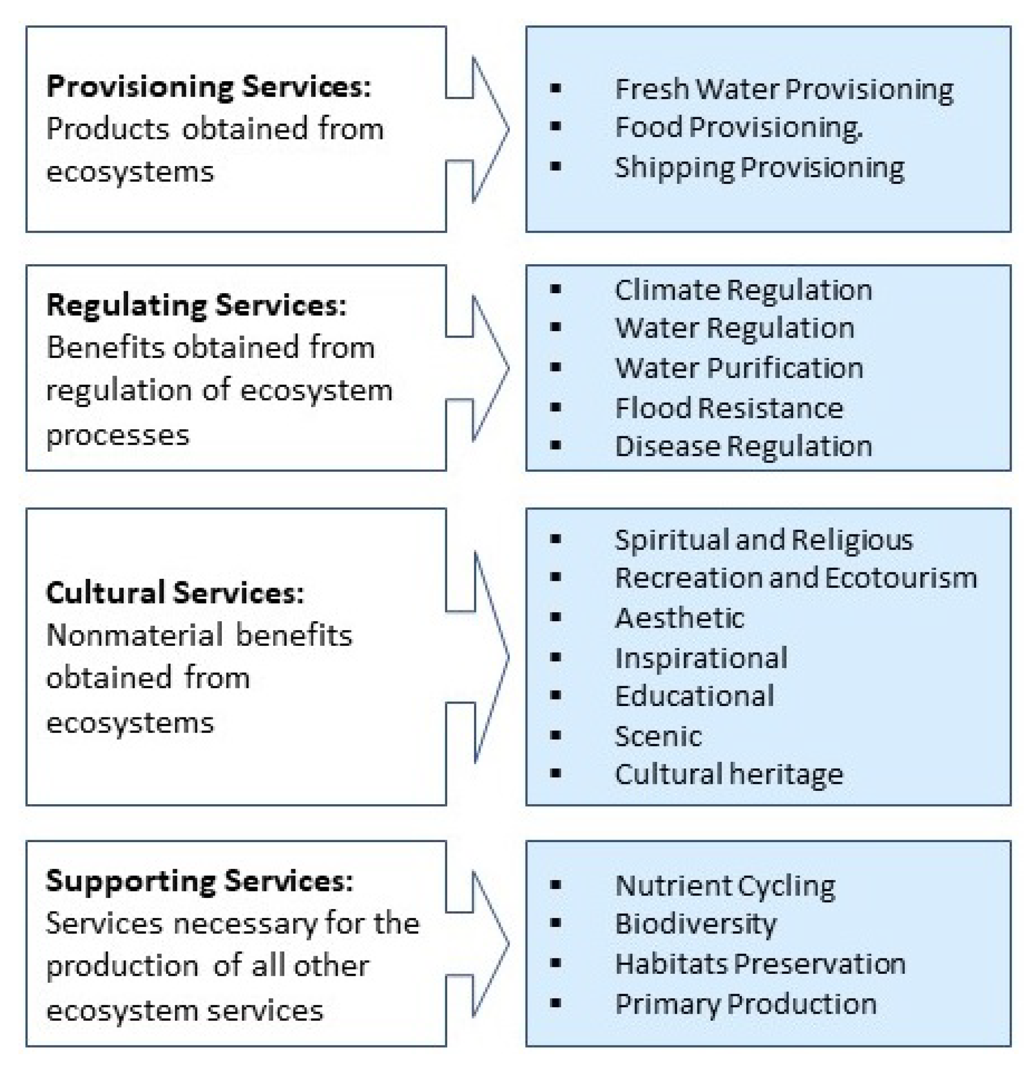
Ecosystem services are defined as the many benefits humans obtain from ecosystems. These include provisioning services such as food and water; regulating services such as flood and disease control; supporting services such as biodiversity maintenance and habitat preservation; cultural services such as entertainment and landscape aesthetics [
1]. The concept of ‘ecosystem services assessment’ has been regarded as a promising way to describe the situation of ecosystem services [
2], scale natural resources storage [
1,
3,
4,
5], manage ecological properties [
6,
7], support natural resources-related policymaking [
8,
9,
10], including freshwater [
11,
12,
13]. As one of the primary provisioning services, water provisioning has become a focus because of its economic and social importance and the increasing scarcity.
Freshwater is becoming scarce worldwide with the rapidly growing population, developing industries, burgeoning agriculture, and increasing consumption [
14,
15,
16,
17,
18]. Climate change and the growing demand for freshwater to support industrial and agricultural development have worsened the situation, and the population suffering from water scarcity has been increasing during the past decades [
19,
20]. Some quantitative indicators mapping the capacity of nature to provide water for human beings were created in quantitative assessment of water provisioning ecosystem services, such as the freshwater provisioning index for humans [
21], and the water security index [
22]. Freshwater scarcity not only impedes economic development and triggers food crises, but also threatens human health since it is directly associated with food quality, energy, and environmental security. To cope with the population explosion and the resulting water shortage, a large variety of ecosystem services related to water resource management have been addressed by assessments [
23,
24,
25]. Economic methods have been flourishing since they were adopted by Costanza [
13,
26,
27,
28,
29,
30], which focus on the economic benefits of ecosystem services and scale it with monetary value. Energy-based methods emerged to mitigate the inaccuracy caused by converting the ecosystem contribution to currency because economic market mechanisms do not always ensure the conservation of ecosystem services [
31,
32]. Investigators attempted to regard ecosystem services as a counterpart of energy flows, such as solar energy [
33,
34]. We adopted the material-based method, which is based on the theory that humans consume ecosystem services via natural resource materials from the ecosystem, such as food, water, wood, oxygen, clean air [
2,
35,
36]. We believe that the process of transferring ecosystem services to humans benefits through some specific carriers. For example, the cropland ecosystems provide food provisioning services, while humans can only obtain and consume this service via obtaining food such as corn and potatoes. Therefore, the weight of the food generated in the cropland ecosystem, which could be measured directly, reflects the amount of food provisioning services [
5]. Similarly, human beings enjoy water provisioning services provided by natural hydrological systems via accessible water. Therefore, water storage in nature can be used to scale water provisioning services.
The capability of remote sensing to perform synoptic, spatially continuous, and frequent observations resulting in large data volumes and multiple datasets at varying spatial and temporal resolutions contributed to spatially explicit ecosystem services assessment [
2,
37,
38,
39,
40]. Compared with the traditional ecosystem services research based on statistical data, remote sensing data can map the spatial distribution of natural resources, mitigating the limitations resulting from administrative boundaries [
41,
42,
43]. However, sound scientific information is critical for making effective environmental policies [
44]. Scientific results should have a scalable maturity that makes them available to the decision-making process. This scalability should correspond to the aggregated level of political units that transforms scientific findings into practical applications. In this paper, we aggregated the assessment results derived from remote sensing data at the county level. We proposed a quantitative approach that reflects the natural situation and provides a promising mechanism for linking scientific information to decision-making via demographic, landscape, and economic statistics based on administrative divisions.
Some of the limitations of existing research can be summarized as follows: (1) While the ecosystem services assessment has made significant progress in recent decades, existing methods largely focus on estimating the total output from ecosystems [
45,
46,
47,
48], which cannot reflect the ecosystems in full-spectrum; they cannot distinguish the ecosystems with the same assessment results but in various sizes. For example, it is unreasonable to equate a lake covering an area of a hundred hectares to another lake covering twenty hectares just because they have the same water provisioning output. They also put the same assessment results on the ecosystems with an opposite trend. For instance, a progressive ecosystem whose assessment result has risen to a certain threshold should be distinguished from a deteriorating ecosystem whose result has fallen to this threshold. (2) In terms of temporal scale, few studies followed a long continuous timeline (over 20 years). Most existing research is limited to a short time period [
2,
49,
50,
51,
52,
53]. (3) From a spatial perspective, most existing studies mapped the spatial distribution of ecosystem services; few studies explored the spatial characteristics and changes over time [
54,
55,
56,
57,
58]. (4) Even though numerous research targets ecosystem services, quantitative relationships between influencing factors and ecosystem services have not been revealed precisely [
59]. (5) Although the potential of remote sensing application in ecosystem services assessment has been explored gradually, the remote sensing-based results are not available at the decision-making level because these results are based on natural boundaries rather than county boundaries [
49,
60,
61,
62], which is challenging to apply in policymaking, measures taken, and practical management. All of the requirements mentioned above call for systematic quantification studies.
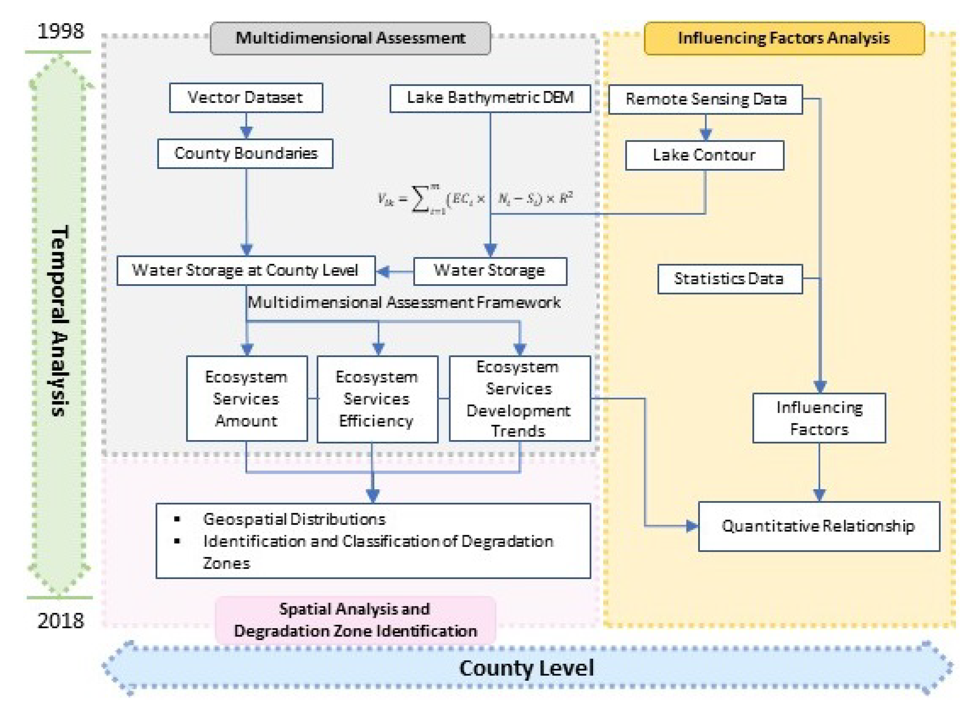
Compared with previous studies, the highlights of this paper are as follows: (1) We expanded the water provisioning ecosystem services assessment from an ‘output’ perspective to an ‘output-efficiency-trend’ multidimensional framework [
5], assessing ecosystem services from outputs, efficiency, and trend simultaneously (see
Figure 1). Thus, some neglected information in traditional single perspective assessment can be revealed. (2) We analyzed 21 years of water provisioning ecosystem services in the study area, characterizing the changes over a long time period. (3) We revealed the spatial distribution characteristics via exploratory spatial analysis methods, identified and classified the degradation zones, and put forward the priorities in lake ecosystem management. (4) We constructed a model to explore the quantitative relationships between the main influencing factors and the multidimensional assessment results. (5) We analyzed the water provisioning services derived from remote sensing data at the county level, making it available to policymakers and natural resource managers as a reference in practical works.
2. Materials and Methods
2.1. Study Area
The state of Minnesota is known for its abundance of surface water bodies, known as the “Land of 10,000 Lakes” [
63]. According to the statistics provided by the Minnesota Department of Natural Resources, there are 11,842 lakes over 4.0 ha in size [
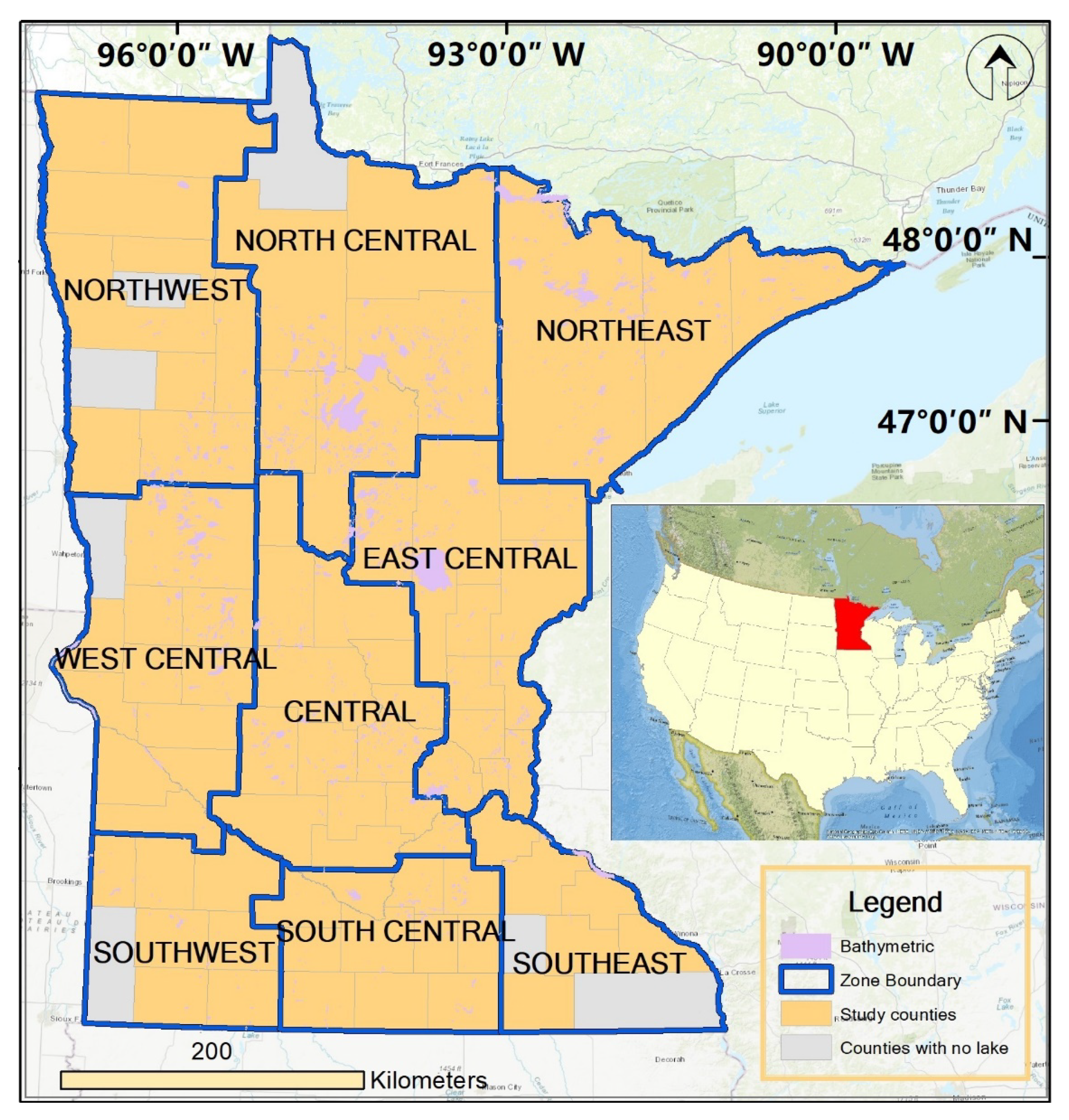
64]. Due to the limited availability of lake bathymetric data, this study focused on 1290 lakes in 70 counties in Minnesota (
Figure 2). The lake areas range from 0.04 ha to 52,426.39 ha, with a total surface water area of 441,363.64 ha (2018). We adopted the regional definition proposed by the Minnesota Department of Agriculture [
65], which divides Minnesota into nine regions: Northwest, North Central, Northeast, West Central, Central, East Central, Southwest, South Central, and Southeast (see
Figure 2).
2.2. Geospatial and Statistical Datasets
The datasets we used in this study include lake bathymetric data, remote sensing products, and demographic and economic data (see
Table 1). More details about each dataset are described below. We derived the influencing factors from remote sensing images at the pixel scale and then aggregated them to the county-level statistics.
2.2.1. Lake Bathymetric Data
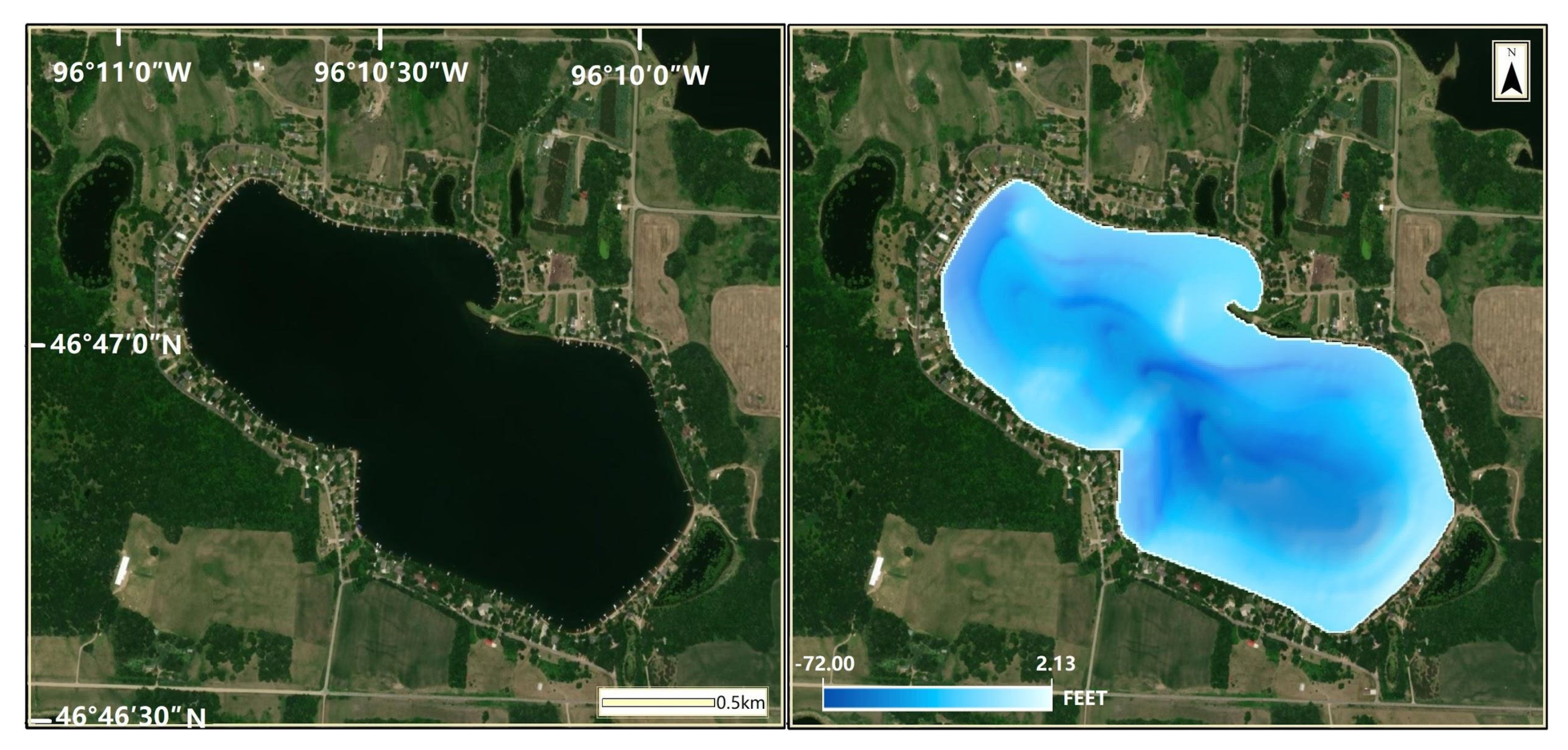
Lake bathymetric data were acquired from the Minnesota Geospatial Information Office [
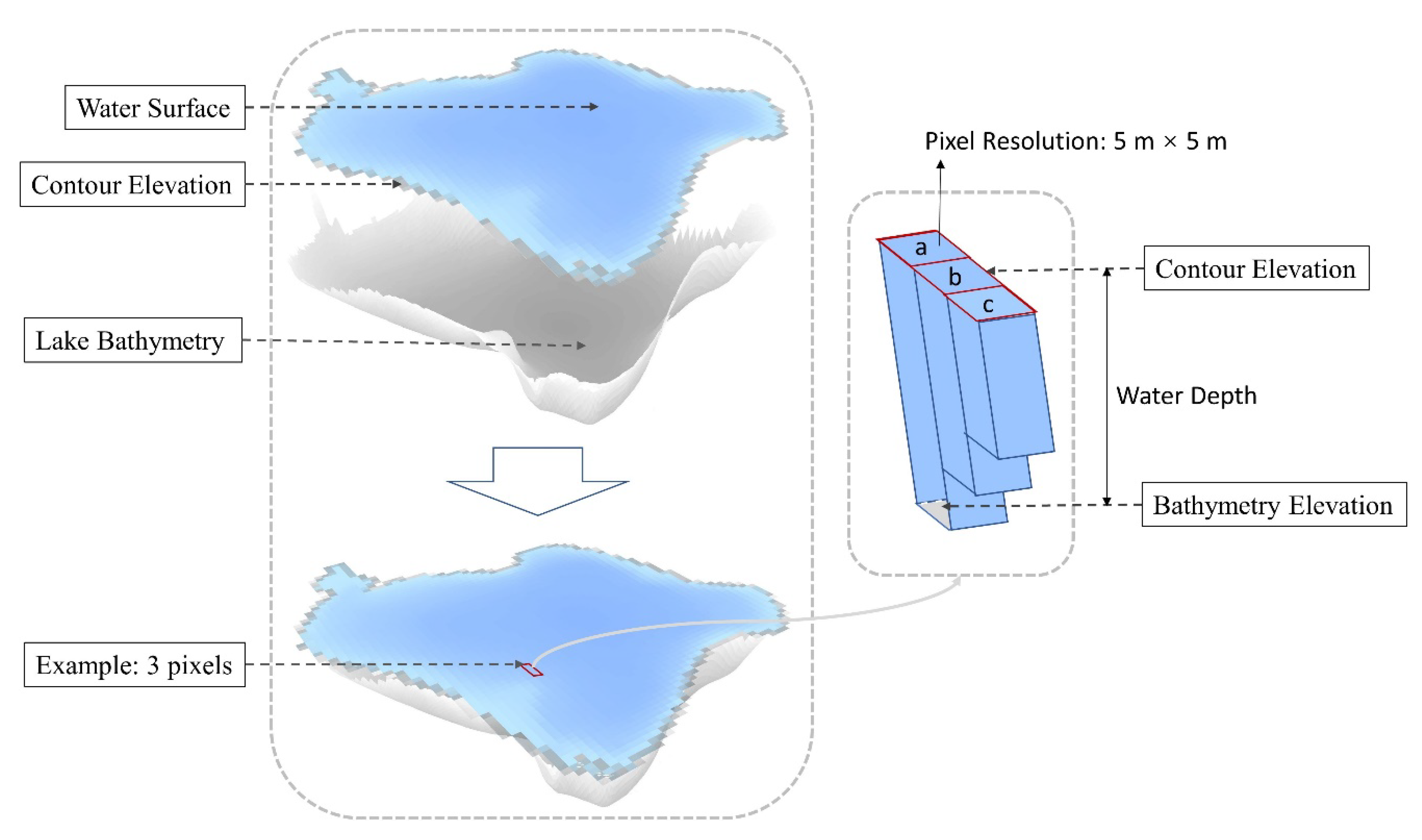
66], which contains lake bathymetric contours, lake bathymetric digital elevation model (DEM), and lake bathymetric outline. The lake bathymetric DEM has a 5 m spatial resolution with one attribute representing lake depth in (negative) feet, covering approximately 1900 lakes. An example of the lake bathymetric DEM is shown in
Figure 3.
2.2.2. Remote Sensing Data
We used various remote sensing products (see
Table 1) to quantify lake water dynamics and explore influencing factors. All of these remote sensing products [
67] and the main data processing are completed on the Google Earth Engine platform. Google Earth Engine is a remote sensing archive with petabytes of data in one location, as well as a cloud-based geospatial processing platform for large-scale data analysis. It is unique in the field as an integrated platform due to the following advantages: (1) The public data catalog has vast amounts of publicly available data including imagery, geophysical, climate and weather, demographic, and vector data. (2) Unprecedented speed resulted from the distributed, cloud-based computing power which reduces processing times by orders of magnitude. (3) The application program interface (code editor) empowers traditional remote sensing scientists, and the graphical user interface (explorer) provides a friendly way to begin exploring and analyzing data for a much wider audience that lacks the technical capacity [
67].
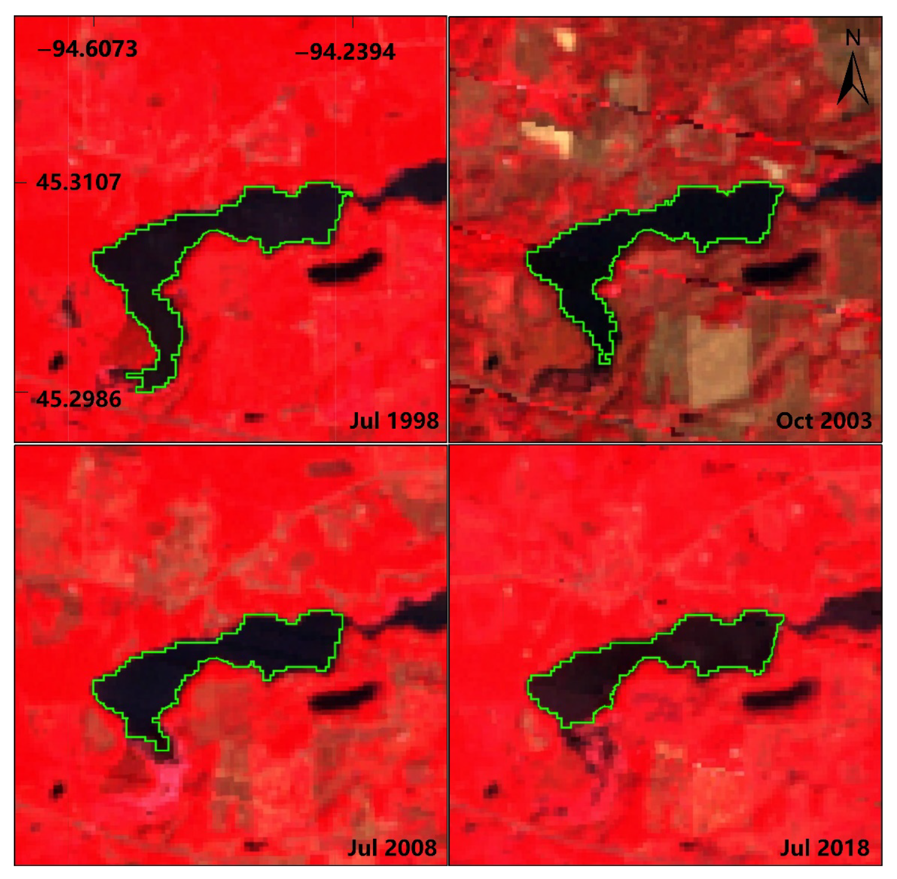
The European Commission’s Joint Research Centre (JRC) Global Surface Water (GSW) was derived from three million Landsat satellite images (i.e., Landsat 5/7/8), recording the months and years when water was present, where occurrence changed and what form changes took in terms of seasonality and persistence at a 30 m resolution from 1984 to 2019 [
68]. Each pixel was individually classified as water/non-water. We derived multi-temporal water surface areas based on the JRC GSW images.
Figure 4 shows examples of lake water areas extracted from Landsat images for the year 1998, 2003, 2008, and 2018, respectively. Each background image shown in
Figure 4 is a false-color composite.
The Penman–Monteith–Leuning Evapotranspiration V2 (PML_V2) products include evapotranspiration (ET) and gross primary product (GPP) at a 500 m spatial resolution with an 8 day temporal frequency from 2002 to 2017. Each PML_V2 imagery consists of five bands, including the gross primary product (GPP), vegetation transpiration (Ec), soil evaporation (Es), interception from vegetation canopy (Ei), waterbody, snow, and ice evaporation (ET_water). We derived the waterbody evaporation, a vital influencing factor, from the ET_water band in this study.
The Daily Surface Weather and Climatological Summaries (Daymet V3) dataset provides gridded estimates of daily weather parameters for the United States. It was derived from selected meteorological station data and various supporting data sources during 1980–2020. Each Daymet V3 imagery has seven bands with a 1 km spatial resolution, including the duration of the daylight period (day1), daily total precipitation (prcp), incident shortwave radiation flux density (srad), Snow water equivalent (swe), Daily maximum 2 m air temperature (tmax), daily minimum 2 m air temperature (tmin), daily average partial pressure of water vapor (vp). As one of the influencing factors of water provisioning ecosystem services, the annual precipitation was derived from the ‘prcp’ band.
The Terra Land Surface Temperature and Emissivity dataset from the United States Geological Survey (USGS) Earth Resources Observation and Science (EROS) Center includes an average 8 day land surface temperature (LST) in a 1 × 1 km2 grid with 12 bands since 2000. We used the ‘day land surface temperature’ band to extract the average daily temperature in 2018 for influencing factor analysis.
The National Land Cover Database (NLCD) is a 30 m Landsat-based land cover database. The ‘landcover’ band, which classified land use into 20 categories, was used to calculate the vegetation coverage rate and the artificial land coverage rate. We identified developed areas (open space, low intensity, medium intensity, and high intensity) as artificial land, forest, grassland, and shrub areas as vegetation coverage land.
2.2.3. Demographic and Economic Data
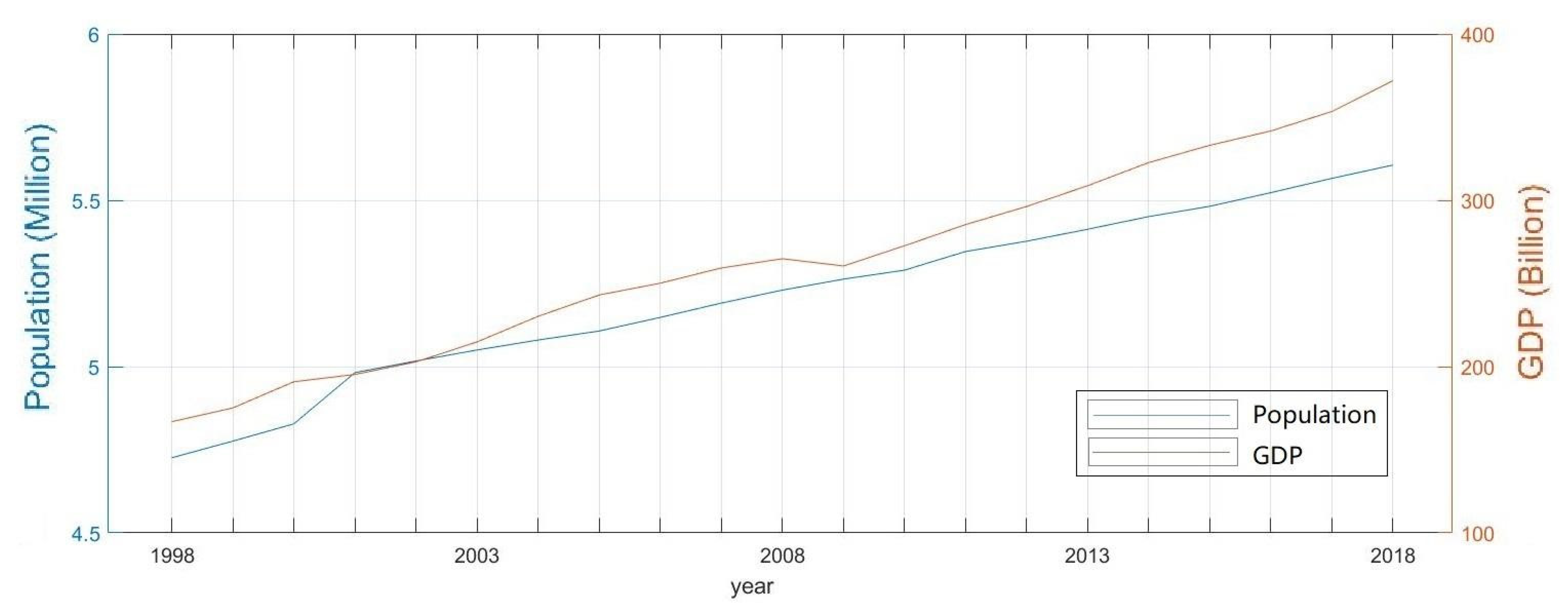
As indicators that directly reflect the intensity of human activities, population, and gross domestic product (GDP) statistics at the county level were obtained from the United States Department of Commerce database [
69].
Figure 5 shows that the population and GDP in Minnesota have been rising steadily since 1998. It was reported that 4,726,411 people lived in Minnesota in 1998, and 20 years later in 2018, the total population increased to 5,608,762, with an annual growth rate of 0.86% (1998–2018). With these new numbers, Minnesota became the 21st most populous state in the US [
70,
71]. The economy of Minnesota produced USD 166.87 billion of gross domestic product in 1998, and it increased to USD 337.22 billion in 2018 [
72,
73], with an annual growth rate of 5.44% (1998–2018) [
74].
2.3. Water Storage Estimation Method
Lakes are one of the most important natural ecosystems, being highly valued for a wide range of ecosystem services. According to the ecosystem services classification proposed by the Millennium Ecosystem Assessment (MA), a lake ecosystem provides provisioning services, regulating services, cultural services, and supporting services (
Figure 6). We focused on the water provisioning ecosystem services of lakes in this study, and water storage is an essential assessment component.
Wu et al. [
75] proposed a new approach for estimating the above-water volume of wetland depressions in the Prairie Pothole Region (PPR) using a contour-tree method with DEMs derived from light detection and ranging (LiDAR) data. The above-water volume (
) of each depression was calculated based on a statistical analysis of the LiDAR DEM cells enclosed by the depression boundary contour:
where
is the elevation of the depression boundary contour;
is the number of cells enclosed by the depression boundary contour;
is the summation of elevation values of all cells enclosed by the contour;
is the spatial resolution of the LiDAR DEM.
We adopted the same method to calculate lake water storage based on the bathymetric data cells with a 5 m spatial resolution. As shown in
Figure 7, the lake water was divided into cuboids based on pixels of DEM, and the above-water volume was calculated by the summation of the volumes of these cuboids. The total lake water storage can be calculated as follows:
where
is the total lake water storage;
is the number of lakes, which is equal to 1290 in this study;
is the contour elevation of lake
;
is the number of cells enclosed by the contour of lake
;
is the summation of bathymetric elevation values enclosed by the contour of lake
;
is the pixel area of bathymetry cells, which is equal to 25 m
2 in this paper.
2.4. A Multidimensional Assessment Framework
The multidimensional ecosystem services assessment framework we proposed in 2020 [
5] explores ecosystem services from multiple perspectives. It focuses on the service output from the natural ecosystems and analyzes the service efficiency and trend simultaneously. It considers the output per unit area among different ecosystems and the changes over time in one ecosystem, which have been largely ignored in the traditional assessment methods.
Ecosystem services are assessed in three dimensions in this framework, including output (P), efficiency (Q), and trend (D). The output is defined as the total amount of ecosystem services provided by natural ecosystems, and it is the total water storage in this research. The ecosystem service efficiency is defined as the proportion of ecosystem services generated per unit area of ecosystem, which is lake surface area in this paper. The trend index indicates the change in ecosystem efficiency, defined as a vector whose direction and magnitude represent the direction and rate of change, respectively. We used the total water storage as the water provisioning output index, the water storage divided by the lake area as the efficiency index, and the water provisioning annual change vector as the trend index in this paper.
We constructed a multidimensional assessment framework based on three axes, output (P axis), efficiency (Q axis), and trend (D axis). We defined eight assessment spaces with various properties in the multidimensional assessment framework. Every object has a unique ecosystem services assessment cuboid, which means how many assessment space properties the object shows in the proposed framework. In
Figure 8a, objects ‘a’ and ‘d’ are in Space 5, ‘b’ is in Space 3, and ‘c’ is in Space 2. Apparently, ‘a’ and ‘d’ share the properties of Space 5, and ‘b’ and ‘c’ share the properties of Space 3 and Space 2, respectively. However, cuboid ‘a’ is much larger than cuboid ‘d’, indicating that ‘a’ has more significant Space 5 properties.
A z-score describes the position of a raw score in terms of its distance from the mean, which is measured in standard deviation units. The z-score is positive if the value is above the mean, and negative if it is below the mean. It allows the comparison of scores on different kinds of variables by standardizing the distribution. A z-score can be calculated by the following formula:
where
is the z-score,
is the mean of the raw scores,
is the standard deviation of the raw scores. Observations are converted to a standard normal distribution via the z-score standardization. The mean of the standardized data is 0, and the standard deviation is 1. At the same time, the position of every object in all observations is revealed. For example, where a z-score is equal to 2, the observation is larger than 97.7% of the overall data. Conversely, when a z-score is equal to −2, the observation is smaller than 97.7% of the overall data (
Figure 8b). We defined P-score, Q-score, and D-score (
Table 2) according to the statistical significance of z-scores to express the regional relative level of ecosystem services in each county.
The multidimensional assessment scores (i.e., P, Q, and D) follow a standard normal distribution. In other words, about 68% of the scores fall within one standard deviation away from the mean; about 95% of the scores fall within two standard deviations; about 99.7% of the scores fall within three standard deviations (see
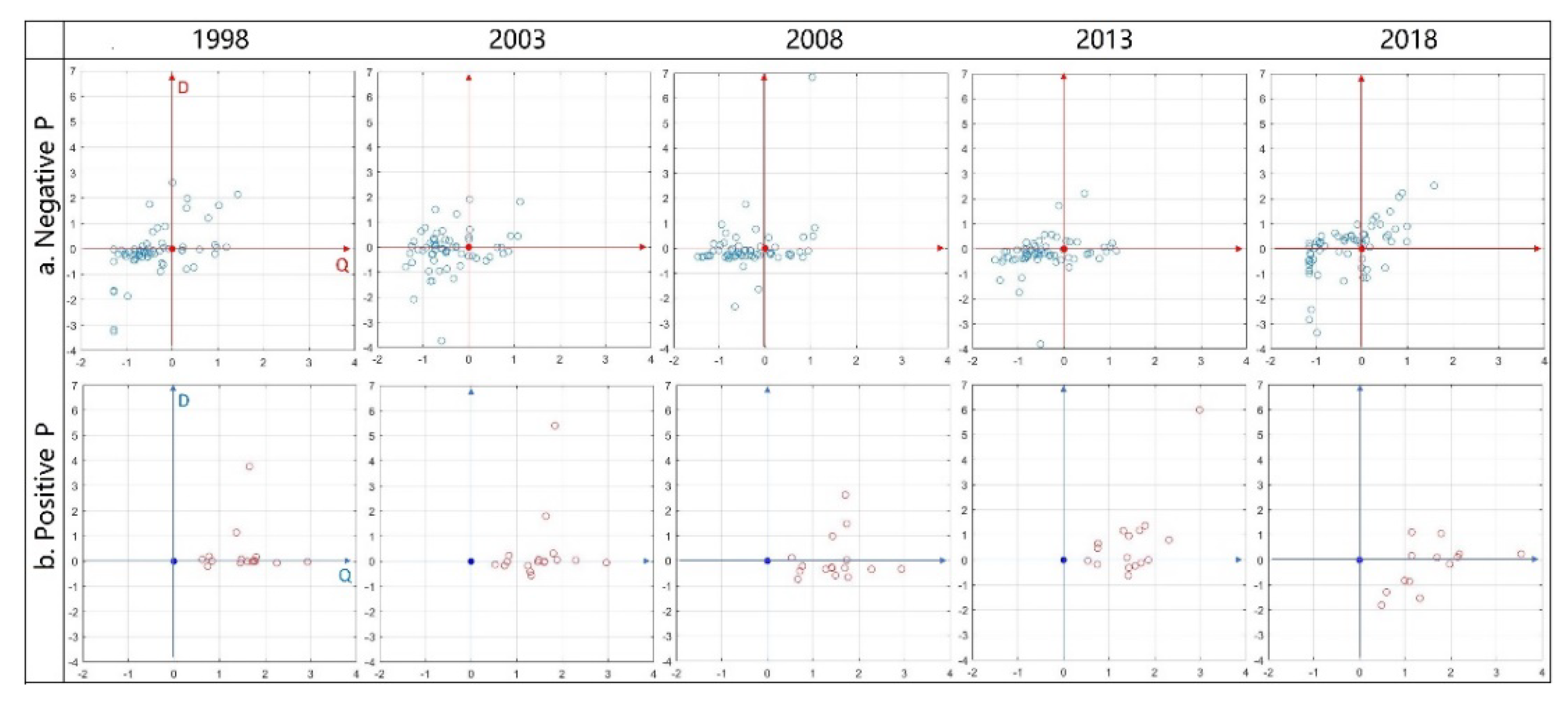
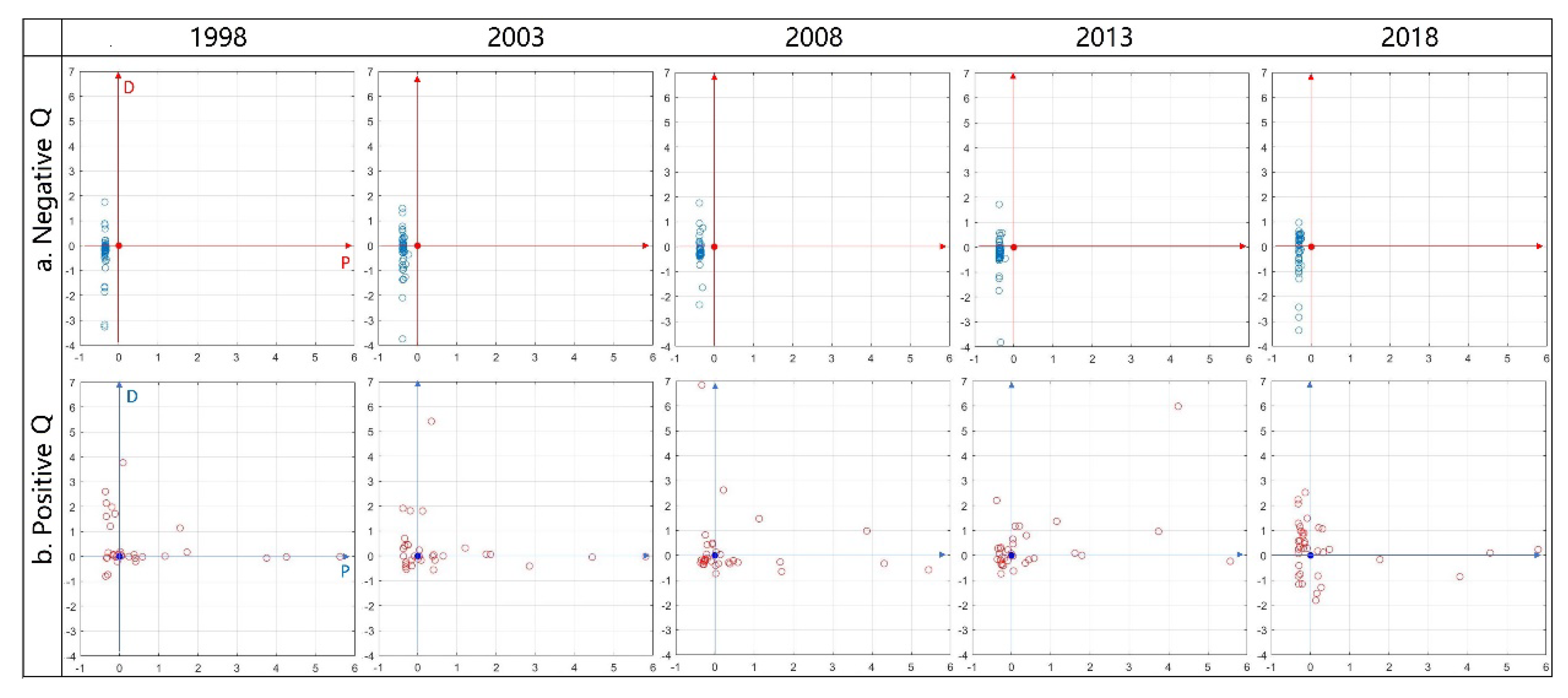
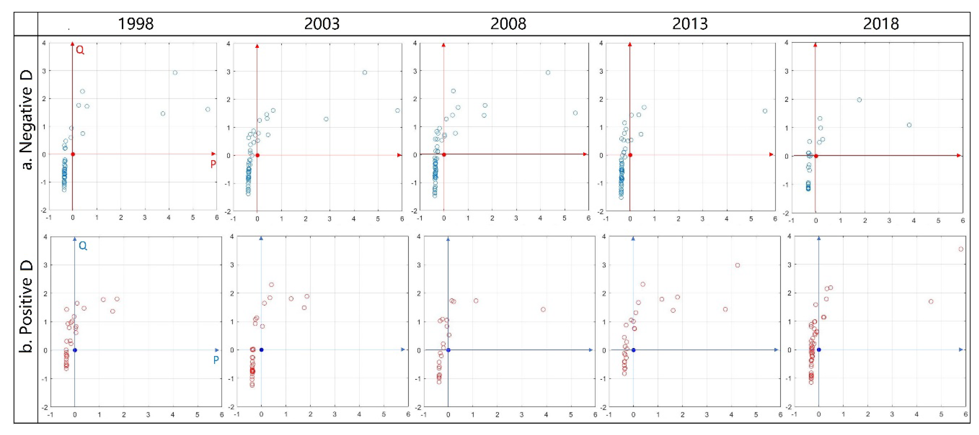
Figure 8b). We identified scores with absolute values greater than three as extreme objects. We then converted the multidimensional assessment results to ‘Q-D,’ ‘P-D,’ ‘P-Q’ distributions by slicing the multidimensional assessment framework on the P, Q, D plane, respectively (
Figure 8c). Bidimensional projections make the relationship between scores and extreme objects easier to be identified. The properties of each assessment space are shown in
Table 3.
2.5. Exploratory Spatial Data Analysis
Much of the groundwork in spatial statistics is concerned with the description and exploration of spatial datasets [
76]. The generic term for such methods in the context of spatial analysis is exploratory spatial data analysis (ESDA). In practical applications, ESDA emphasizes the natural distribution of spatial data, focusing on the correlation of events, inheriting the quantitative geographic analysis methods, and exploring the spatial patterns of data [
77].
Spatial clustering is the grouping of spatial datasets, with maximized intra-group similarities and the differences among groups, which is an efficacious method for spatial distribution identification and outlier detection. Some traditional methods such as Moran’s I analysis, hotspot analysis, and grouping analysis are used frequently in spatial clustering analysis. We used hotspot analysis, supported by the Getis–Ord
Gi* statistic, to identify statistically significant clusters of high values (hot spots) and low values (cold spots) in this study.
Gi* is positive for a ‘hot spot’ and negative for a ‘cold spot’. The Getis–Ord
Gi* statistic with n observations
can be calculated using the following formula:
where
is the mean of the observations
,
is the spatial weight between
and
,
.
The z-scores and
p-values derived from the hotspot analysis are measures of statistical significance indicating whether or not to reject the null hypothesis that the values analyzed have a random spatial distribution. In effect, they indicate whether the observed spatial clustering of high or low values is more pronounced than one would expect in a random distribution of the same values. The critical
p-values and z-scores are shown in
Table 4.
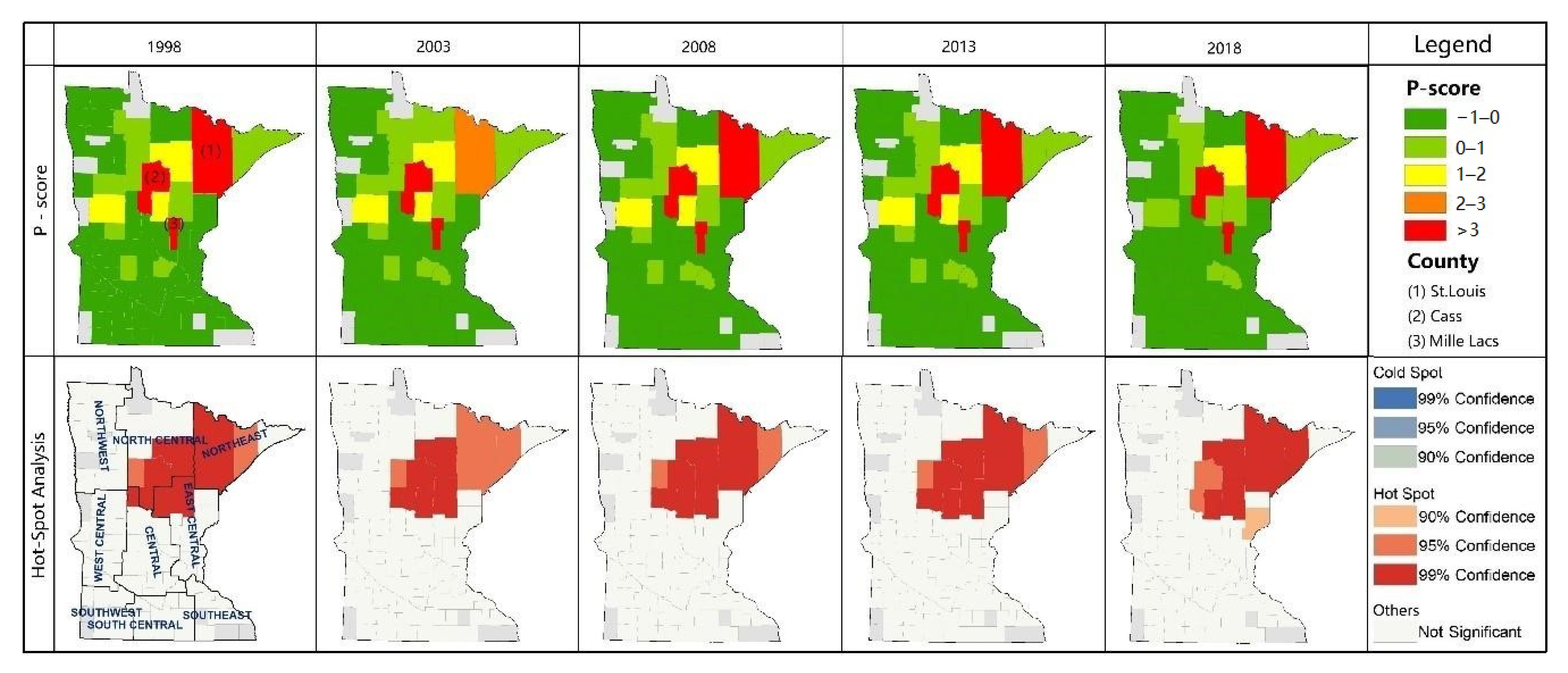
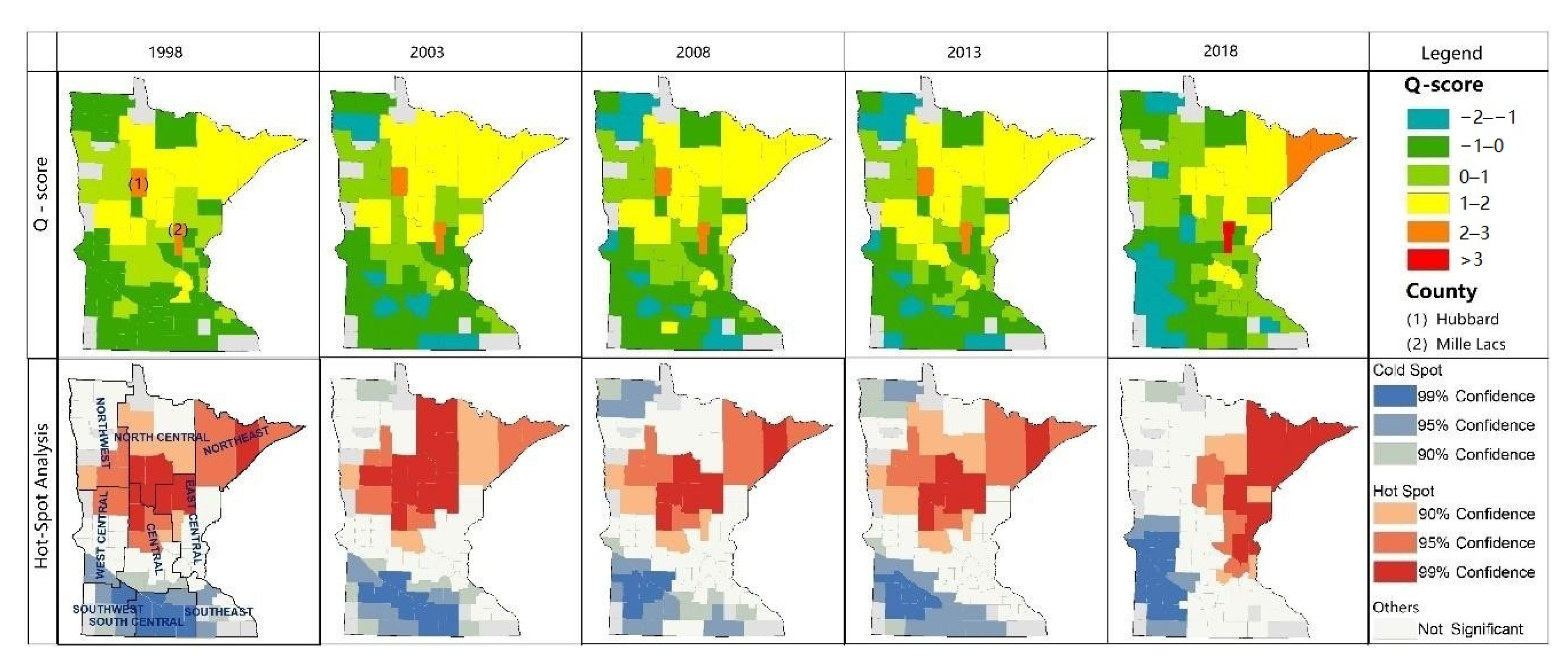
We analyzed P-scores, Q-scores, and D-scores using exploratory spatial data analysis methods to describe the spatial distribution of ecosystem services output, efficiency, and development trend, respectively.
2.6. Principal Components Regression
Principal components regression (PCR) is a technique for analyzing multiple regression data that suffer from multicollinearity. When multicollinearity occurs, least squares estimates are unbiased, but their variances are large so they may be far from the true value. The theory of PCR is to eliminate multicollinearity of original variables using principal component analysis. The principal component variables are used as independent variables in the regression model, and then they are substituted with the original variables according to the score coefficient matrix to the regression model obtained. The principal components regression model with n sets of observations and
k original variables
can be outlined as follows:
First, complete a principal components analysis of the
X matrix and save the principal components in
Z. We then transform the original variables to their principal components as:
where
is a diagonal matrix of the eigenvalues of
,
is the eigenvector matrix of
, and
is a data matrix made up of the principal components.
is orthogonal so that
.
Second, fit the regression of
Y on
Z obtaining least squares estimates of
A.
Third, set the last element of
A equal to zero and transform back to the original coefficients using
B =
PA. The two sets of regression coefficients,
A for principal components and
B for original variables, are related using the formulas
Last, the F test is adopted to test the statistical significance of the principal component regression model in this study.
2.7. Mann–Kendall Test and Sen’s Slope Estimator
The Mann–Kendall test is used to determine whether a time series has a monotonic upward or downward trend. It does not require that the data be normally distributed or linear. It does require that there is no autocorrelation. The null hypothesis for this test is that there is no monotonic trend in the series. The alternate hypothesis is that a trend exists. This trend can be positive, negative, or non-null. The Mann–Kendall test with n sets of a time series can be expressed as follows:
If
, the later observations in the time series tend to be larger than those that appear earlier in the time series, and vice versa. It has been documented that when
, the statistic
S is approximately distributed with the mean
. The variance statistic is given as:
where
is the number of ties up to sample
i, the Mann–Kendall test statistics
is defined as follows:
follows a standard normal distribution here. When , the original time series signifies an upward trend, and vice versa. Suppose we want to test the null hypothesis : There is no monotonic trend in a time series, versus the alternative hypothesis : There is a statistically significate downward or upward trend. Given a confidence level , would be rejected if , which means the time series would be supposed to experience a statistically significant trend, where is the corresponding value of following the standard normal distribution. On the contrary, would be rejected if , which means there is no monotonic trend in the time series.
In addition, the magnitude of a time series trend can be evaluated by a simple non-parametric procedure developed by Sen. The trend is calculated by:
where
is Sen’s slope estimate.
indicates an upward trend in a time series,
significates a downward trend.
4. Discussion
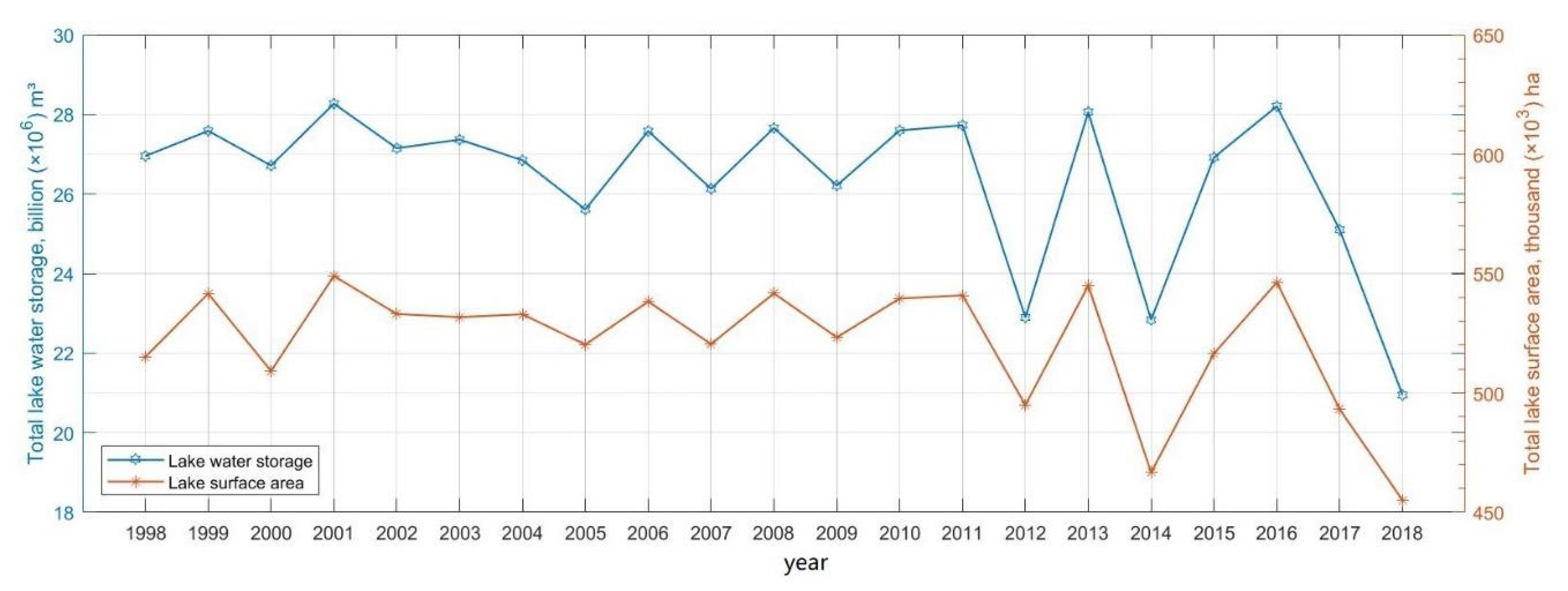
We analyzed the lake water provisioning services in Minnesota from both spatial and temporal perspectives. The temporal analysis shows that lake water storage in Minnesota fluctuated over time from 1998 to 2018 with an increasing interference, which is consistent with the results of the Lake Hydrology Program [
78]. According to Minnesota’s water supply report by the Minnesota Department of Natural Resources Waters [
79] and Minnesota water use report by the University of Minnesota Water Resources Center, surface water plays an essential role in water provisioning in Minnesota, such as public water supply and irrigation, and cooling in power generation. About 18.6% of the water comes from groundwater, and the remaining water used comes from surface water. They also found a growing consumption of surface water, which could contribute to the increasing disturbance we found in this study.
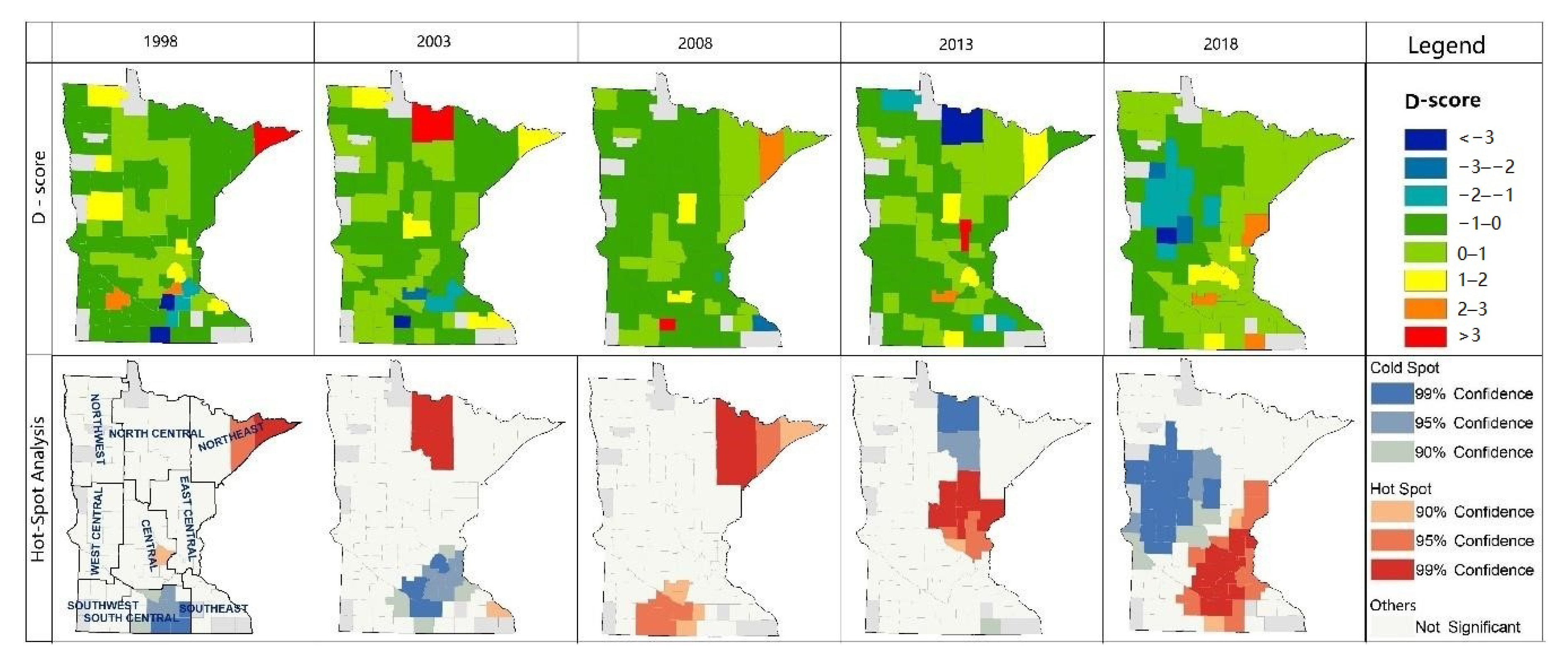
Water provisioning output, efficiency, and trend have relatively stable spatial distribution, while the clustering patterns are different: (1) The high-value output zones are located in Northeast Minnesota, including Northeast, North Central, and East Central, dominated by forests. This distribution does not necessarily match the demand distribution for agricultural and industrial water use. We should consider the availability of abundant water provisioning for agricultural and industrial processing in the development plan. Only one high-value cluster in water provisioning output indicates that the water provisioning output is sound in total; there is no large-scale water shortage area. (2) Efficiency represents the water provisioning capacity per unit surface water ecosystem. The spatial distribution is similar to the output; high values are concentrated in Northeastern Minnesota. Thus, the spatial mismatch between supply and demand also exists in the distribution of efficiency. Unlike the output, the low-value clusters are significantly inefficient, which means the water provisioning capacity per unit of surface water is flimsy, where the below-average zones frequently appear considerably. (3) Compared with the above two indicators, the trend index distribution is largely random. However, the low-value area significantly expanded, so as the hot spots and cold spots. It shows that the water provisioning trend index declines over time, the below-average area expands, and extreme values are gathering considerably.
Projections from co-ordinate planes defined by assessment dimensions prove water provisioning efficiency is positively dependent on output, where output is above-average, the efficiency is above-average, too. While output is negatively dependent on efficiency, where efficiency is below-average, the output is below-average also. These correlations should be considered in surface water resources management and ecosystem protection projects.
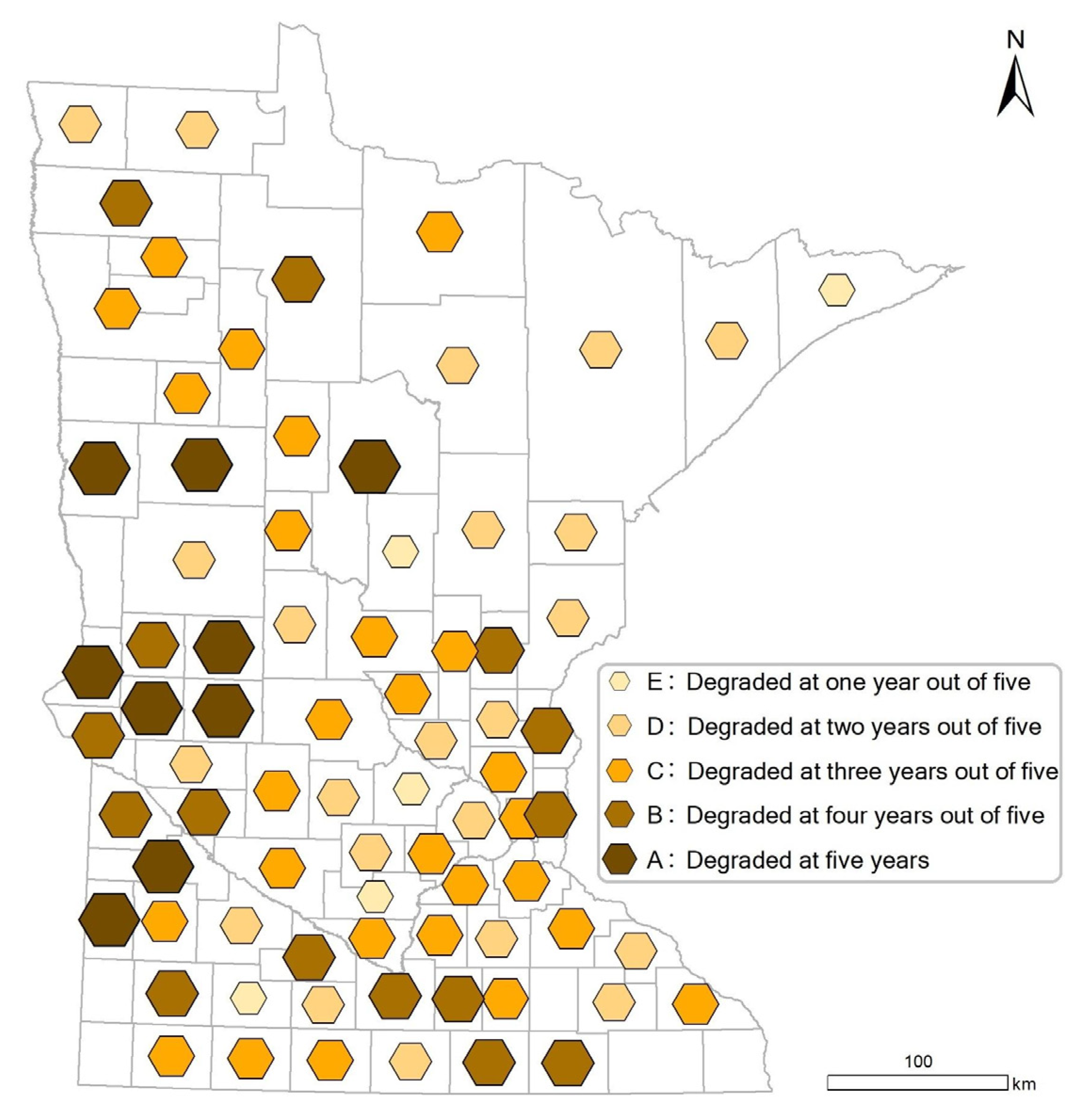
We identified nine counties, including Becker, Cass, Clay, Douglas, Lincoln, Pope, Stevens, Transverse, and Yellow Medicine, where water provisioning service is degrading in the five studied years and fifteen counties degraded for four out of five years. Counties with severe water provisioning degradation are mainly concentrated in three zones (Northeast, East Central, and Southeast) in Western Minnesota. The degradation area distribution is consistent with the distribution of cropland in Minnesota, while it does not match the population and industry distribution. Agricultural activities have proved to be highly dependent on surface water availability [
80]. Simultaneously, the human disturbances to surface water are strong where the agricultural activities are vigorous, such as dam water storage and irrigation drainage [
81,
82,
83]. Thus, it is reasonable that prosperous agricultural production is primarily responsible for the degradation of water provisioning services in Western Minnesota, compared with the population or industrial activities.
The quantitative model between the influencing factors and the assessment results show that human activities have a more substantial impact on water provisioning output than natural climate factors, which reminds us that protecting the total water storage and developing the economy is fundamentally an organic unity and complement each other. The climate factors, especially temperature and precipitation, have more substantive impact on water provisioning efficiency and trend. It confirms that combat climate change measures are essential for improving water provisioning efficiency and intervening in its trends.
We conducted this comprehensive study based on remote sensing products and lake bathymetric data, analyzed the characteristics of water provisioning development of 70 counties in Minnesota from temporal and spatial perspectives, interpreted ecosystem services from multiple dimensions and quantitatively explored their influencing factors. Nevertheless, the study has some limitations: (1) Due to the limited availability of lake bathymetric data, some lakes without lake bathymetric data were not included in the analysis, which might result in some deviations between the county-level analysis and the actual situation. (2) We only selected five time periods (i.e., 1998, 2003, 2008, 2013, and 2018) as the representative years to explore the spatial characteristics of water provisioning ecosystem services at the county level. It should be noted that each time period is just one snapshot in time, which might not capture the changes between the representative years. (3) The natural ecosystems are dynamic complexes of plants, animals, micro-organism communities, and non-living environments interacting as functional units [
84]. Their mechanisms and functional processes are complicated and correlated. We adopted a linear model to simulate the various influencing factors, which can reflect the function intensity of influencing factors, but it cannot simulate or express the specific process and its mechanism of influencing factors. (4) Our proposed framework highlights water storage as the main factor affecting lake ecosystem services. However, there are other factors (e.g., water quality, air quality, local climate regulation, aesthetics) that may also significantly affect lake ecosystem services [
85,
86]. Due to the lack of relevant data at the individual lake level, we did not integrate these factors into our framework. Future research can focus on applying the multidimensional ecosystem service assessment framework to other ecosystem services and exploring models that simulate real processes of how influencing factors work.
5. Conclusions
We conducted a comprehensive, long-term, multidimensional ecosystem service assessment that can potentially benefit policymakers. First, we revealed some neglected degradations in traditional output-based assessment, such as the water provisioning capacity per unit of surface water is flimsy, and the number of counties with degradation is increasing. Second, we identified the relatively stable distribution of water provisioning services during 1998–2018 and the various spatial clustering patterns from three dimensions. Third, we revealed the dependence between high-level efficiency and high-level output, low-level output, and low-level efficiency, which could potentially be used in the water resources utilization and ecosystem service management. Fourth, we identified nine severely degraded counties and revealed that the Western Minnesota counties are more degraded than the others, which is particularly important to the sustainable ecosystem utilization and ecological services enhancement. Last but not least, we modeled the relationships between the principal influencing factors and the multidimensional assessment results, which reveals that human activities impact water provisioning services in Minnesota more than climate changes.
In summary, the contributions of this study are as follows: First, we expanded the perspective of ecosystem services assessment from ‘output’ to an ‘output-efficiency-trend’ multidimensional framework, measuring the provisioning capacity of ecological services per unit area of the ecosystem and the trend while assessing the output. Thus, we revealed some degradations which could not be identified in traditional output perspective assessment. Secondly, we identified the priorities for policymakers to underpin better protection of lake ecosystems; the higher the degradation level of a county, the higher the priorities it should have. Finally, we revealed that human activities have a more substantial impact than climate change on output and should be paid more attention to output enhancing policy formulation and management implementation. While efficiency and trend are more sensitive to climate changes than human activities, combat climate-changing measures are essential for improving efficiency and development.


