Comparing Three Remotely Sensed Approaches for Simulating Gross Primary Productivity over Mountainous Watersheds: A Case Study in the Wanglang National Nature Reserve, China

Abstract

Light Use Efficiency (LUE), Vegetation Index (VI)-based, and process-based models are the main approaches for spatially continuous gross primary productivity (GPP) estimation. However, most current GPP models overlook the effects of topography on the vegetation photosynthesis process. Based on the structures of a two-leaf LUE model (TL-LUE), a VI-based model (temperature and greenness, TG), and a process-based model (Boreal Ecosystem Productivity Simulator, BEPS), three models, named mountain TL-LUE (MTL-LUE), mountain TG (MTG), and BEPS-TerrainLab, have been proposed to improve GPP estimation over mountainous areas. The GPP estimates from the three mountain models have been proven to align more closely with tower-based GPP than those from the original models at the site scale, but their abilities to characterize the spatial variation of GPP at the watershed scale are not yet known. In this work, the GPP estimates from three LUE models (i.e., MOD17, TL-LUE, and MTL-LUE), two VI-based models (i.e., TG and MTG), and two process-based models (i.e., BEPS and BEPS-TerrainLab) were compared for a mountainous watershed. At the watershed scale, the annual GPP estimates from MTL-LUE, MTG, and BTL were found to have a higher spatial variation than those from the original models (increasing the spatial coefficient of variation by 6%, 8%, and 22%), highlighting that incorporating topographic information into GPP models might improve understanding of the high spatial heterogeneity of the vegetation photosynthesis process over mountainous areas. Obvious discrepancies were also observed in the GPP estimates from MTL-LUE, MTG, and BTL, with determination coefficients ranging from 0.02–0.29 and root mean square errors ranging from 399–821 gC m⁻²yr⁻¹. These GPP discrepancies mainly stem from the different (1) structures of original LUE, VI, and process models, (2) assumptions associated with the effects of topography on photosynthesis, (3) input data, and (4) values of sensitive parameters. Our study highlights the importance of considering surface topography when modeling GPP over mountainous areas, and suggests that more attention should be given to the discrepancy of GPP estimates from different models.

1. Introduction

Understanding the terrestrial carbon cycle is crucial for adaptation to global climate change [1]. Gross primary productivity (GPP), defined as the total amount of carbon fixed by the vegetation photosynthesis process per unit of time and space, is an essential component of the terrestrial carbon cycle [2]. As the main mechanism for terrestrial ecosystems to absorb atmospheric carbon dioxide, a small variation in GPP would significantly influence the carbon balance of ecosystems [3]. Obtaining accurate GPP estimates plays an important role in assessing the terrestrial carbon budget and understanding the responses of terrestrial ecosystems to global climate change [4].

Currently, the globally distributed eddy covariance (EC) systems can only provide GPP estimates over a limited spatial context due to the representation of carbon footprints [5]. Fortunately, the availability of satellite observations make it feasible to acquire important information about ecosystem components at a large scale [6,7]. Various ecosystem models have been developed to obtain spatially-continuous GPP estimates, which can predominantly be categorized as Light Use Efficiency (LUE) models, Vegetation Index (VI) -based models, and process-based models. However, most of these GPP models overlook the effect of topography on the vegetation photosynthesis process [8,9,10,11,12], and limited attention has been given to carbon modeling over mountainous areas. The topographic characteristics of mountainous areas, such as steep slopes, altitude variation, and landscape fragmentation, greatly influence surface energy and hydrologic processes [13,14,15,16], and thus affect the vegetation photosynthesis process [17,18,19,20,21]. Over the last decade, Xie and Li (2020) [22,23] and Govind et al. (2009) [18] have made efforts to improve GPP estimations from LUE, VI-based, and process-based models over mountainous areas, respectively.

LUE models are developed from the radiation conversion efficiency concept [24] and have been widely adopted to generate time-series of regional and global GPP products [25,26,27]. Most LUE models are big-leaf models with the assumption that the whole canopy can absorb direct and diffuse solar radiation simultaneously, such as the Moderate-resolution Imaging Spectroradiometer (MODIS) GPP model (MOD17) [8], Vegetation Photosynthesis Model [28], and EC-LUE [9]. However, many studies have suggested that the treatment of sunlit and shaded leaves should be different in LUE models [10,29,30,31,32]. Sunlit leaves, which absorb both direct and diffuse radiation, are easily light-saturated, and thus their photosynthetic capacity is more constrained by low LUE. In contrast, the photosynthetic capacity of shaded leaves, which only absorb diffuse radiation, is normally constrained by low absorbed photosynthetically active radiation (APAR). To separate the treatment of sunlit and shaded leaves, He et al. (2013) [33] proposed a two-leaf LUE model (TL-LUE) by combining the MOD17 model and the Boreal Ecosystem Productivity Simulator (BEPS) [29,34]. The performance of TL-LUE has been validated for various vegetation types [35,36,37], but neglects topographic characteristics over mountainous areas. To address this problem, Xie and Li [22] developed a mountain TL-LUE model (MTL-LUE) by considering (1) the variation of direct radiation resulting from the different geometric relationships between the tilt of the ground surface and the solar position [38,39,40,41], (2) the shielding of diffuse radiation caused by the tilt of the ground surface itself and surrounding terrain [38,40,41,42], and (3) the alteration of sunlit canopy area due to the different relative positions of geotropic trees [43,44,45]. The GPP estimates from the MTL-LUE model proved to better match the tower-based GPP than those from the TL-LUE model at a mountainous site [22].

VI-based models usually estimate GPP by exploring its direct correlation with remotely sensed green vegetation indices [11], such as the normalized difference vegetation index (NDVI) and enhanced vegetation index (EVI). If GPP was able to be calculated entirely from remotely sensed data, it would be more convenient to have spatially and temporally continuous GPP estimates over larger-scale areas due to the development of the satellite remote-sensing technology. Sims et al. (2008) [12] developed a temperature and greenness (TG) model based on the direct relationship between GPP and the combination of EVI and MODIS land surface temperature (LST), and its satisfying performance has been confirmed by various studies [12,46,47,48,49,50]. In the model application of TG, EVI can be obtained from MODIS (~250 m) or Landsat spectral bands (~30 m), while LST is always provided by MODIS products at the spatial resolution of ~1 km. However, the ~1 km resolution MODIS LST product may lose a large portion of topographic characteristics over mountainous areas [51], and thus the TG model is more suitable for relatively flat areas. To improve the GPP estimation from TG, Xie and Li [23] proposed a mountain TG model (MTG) by adding (1) an elevation-corrected factor for the effect of elevation on temperature [52,53] and (2) a radiation-corrected factor for the contribution of the incoming solar radiation to the spatial variations of temperature [52,54]. MTG has presented a better ability to capture the GPP variations than the TG model at sixteen mountainous sites [23].

Process-based models, such as the BEPS model [29,34], the Biome-BGC model [55], and the Integrated Biosphere Simulator (IBIS) model [56], always use biological, climatic, and soil variables to describe the major components of ecological processes related to vegetation photosynthesis. However, most process-based models overlook the large spatial variation in GPP caused by impacts of topography on received radiation, temperature, and soil water. To improve GPP estimations from process-based models over mountainous areas, Govind et al. (2009) [18] developed an eco-hydrological model (BEPS-Terrainlab, BTL) by integrating the BEPS model with a spatially distributed hydrological model called TerrainLab. BEPS is a two-leaf process-based model, with daily canopy-level photosynthesis simulated by up-scaling Farquhar’s leaf-level biochemical model [57]. Over the past two decades, the BEPS model has been adopted as an effective tool to simulate the carbon and water fluxes between terrestrial ecosystems and the atmosphere in China [58,59,60], North America [61], Canada [62,63], East Asia [64], Europe [65], and the globe [66,67]. TerrainLab was designed to obtain accurate estimations of the water table and soil moisture content in mountainous areas through the use of a subsurface saturated flow mechanism. The TerrainLab model not only considers topographic effects on the spatial distributions of climatic variables, but also describes the movement of soil water by assuming that each pixel is connected to its surrounding eight pixels. The improvement of BTL in simulating carbon and water fluxes over BEPS was proved in a mountainous watershed [18].

Generally, GPP estimation at a site scale is always limited by its spatial representation, whereas a watershed-scale GPP estimation could provide spatial-continuous information on vegetation photosynthesis. The GPP estimates from the above three mountain GPP models (i.e., MTL-LUE, MTG, and BTL) have been proven to match better with tower-based GPP than those from the original models (i.e., TL-LUE, TG, and BEPS) at the site scale [22,23]. However, the discrepancies among the three mountain GPP models, and their abilities to characterize spatial variation in GPP at the watershed scale, are not yet known. BTL considers the combined spatial effect of various environmental indicators and ecological processes on GPP estimation, but its complicated model structure requires a large number of input data and ecological parameters. MTL-LUE has a relatively simple model structure and only considers the process of radiation conversion, and it also requires meteorological data as input. Although the understanding of the vegetation photosynthesis process in MTG is not as detailed as that in BTL and MTL-LUE, MTG has the advantage of extensive remotely sensed information (i.e., estimating GPP without ground data). Therefore, MTL-LUE, MTG, and BTL have different scopes of application.

The MTL-LUE, MTG, and BTL models are developed from different model structures, and use different modeling strategies to describe the complex effect of topography on the vegetation photosynthesis process. The main aims of this study are to: (1) investigate the improvement in the MTL-LUE, MTG, and BTL models over the original models (i.e., TL-LUE, TG, and BEPS) at the watershed scale, (2) compare the GPP estimates from MTL-LUE, MTG, and BTL models at the watershed scale, and (3) analyze and compare the responses of the three mountain GPP models to surface topography (i.e., elevation, slope, aspect, and SVF). This study was carried out in a mountainous watershed, and the outcomes can serve as an example, and the first application, for watershed-scale carbon modeling over mountainous areas.

2. Materials and Methods

2.1. Model Description for GPP Estimation

This work adopted three approaches for simulating gross primary productivity (GPP) over mountainous areas, including three LUE models (i.e., MOD17, TL-LUE, MTL-LUE), two VI-based models (i.e., TG and MTG), and two process-based models (i.e., BEPS and BTL). Detailed descriptions of MOD17 [8], TL-LUE [33,35], MTL-LUE [22], TG [12], MTG [23], BEPS [29,34], and BTL [18] can be found in the literature.

2.1.1. LUE Models

The GPP estimates from MOD17 (GPP_MOD17), TL-LUE (GPP_TL-LUE), and MTL-LUE (GPP_MTL-LUE) can be described as:

$$GP{P}_{MOD17}={\epsilon }_{mtotal}\times APA{R}_{total}\times f(VP{D}_{daytime})\times g(T_{\min })$$

(1)

$$GP{P}_{TL-LUE}=\left({\epsilon }_{msun}\times APA{R}_{sun-ft}+{\epsilon }_{mshd}\times APA{R}_{shd-ft}\right)\times f(VP{D}_{daytime})\times g(T_{\min })$$

(2)

$$GP{P}_{MTL-LUE}=\left({\epsilon }_{msun}\times APA{R}_{sun-mt}+{\epsilon }_{mshd}\times APA{R}_{shd-mt}\right)\times f(VP{D}_{daytime})\times g(T_{\min })$$

(3)

$$g(T_{\min })=\{\begin{array}{c}\begin{array}{cc}\hspace{1em}0\hspace{1em}\hspace{1em}\hspace{1em}\hspace{1em}\hfill & T_{\min }\le T_{\min -\min }\end{array}\hfill \\ \begin{array}{cc}\frac{T_{\min }-T_{\min -\min }}{T_{\min -\max }-T_{\min -\min }}\hfill & \hspace{1em}{T}_{\min -\min }<T_{\min }<T_{\min -\max }\hfill \end{array}\\ \begin{array}{cc}\hspace{1em}1\hspace{1em}\hspace{1em}\hspace{1em}\hspace{1em}\hfill & T_{\min }\ge T_{\min -\max }\end{array}\hfill \end{array}$$

(4)

$$f(VP{D}_{daytime})=\{\begin{array}{c}\begin{array}{cc}\hspace{1em}0\hspace{1em}\hspace{1em}\hspace{1em}\hspace{1em}\hfill & VP{D}_{daytime}<VP{D}_{\max }\end{array}\hfill \\ \begin{array}{cc}\frac{VP{D}_{\max }-VP{D}_{daytime}}{VP{D}_{\max }-VP{D}_{\min }}& \hspace{1em}VP{D}_{\min }<VPD<VP{D}_{\max }\end{array}\\ \begin{array}{cc}\hspace{1em}1\hspace{1em}\hspace{1em}\hspace{1em}\hspace{1em}\hfill & VP{D}_{daytime}>VP{D}_{\min }\end{array}\hfill \end{array}$$

(5)

where ε_mtotal, ε_msun, and ε_mshd are the maximum LUE of the total canopy, sunlit leaves, and shaded leaves, respectively; f(VPD_daytime) and g(T_min) are the scalars of daytime VPD and the minimum air temperature (T_min); T_min-min, T_min-max, VPD_max, and VPD_min are the model parameters that are specific to vegetation types; APAR_total, APAR_sun (or APAR_sun-ft, APAR_sun-mt), and APAR_shd (or APAR_shd-ft, APAR_shd-mt) are the APAR of the total canopy, sunlit leaves, and shaded leaves, which can be calculated as:

$$APA{R}_{total}=PA{R}_{total}\times (1-e^{-k\times LA{I}_{total}})$$

(6)

$$APA{R}_{sun}=(1-\alpha )\times (PA{R}_{dir}\times \frac{\cos (\beta )}{\cos ({\theta }_{local})}+\frac{PA{R}_{dif}-PA{R}_{difu}}{LA{I}_{total}}+C)\times LA{I}_{sun}$$

(7)

$$APA{R}_{shd}=(1-\alpha )\times (\frac{PA{R}_{dif}-PA{R}_{difu}}{LA{I}_{total}}+C)\times LA{I}_{shd}$$

(8)

$$PA{R}_{difu}=PA{R}_{dif}\times \exp \left(\frac{-0.5\times \Omega \times LA{I}_{total}}{0.537+0.025\times LA{I}_{total}}\right)$$

(9)

$$C=0.07\times \Omega \times PA{R}_{dir}\times \left(1.1-0.1\times LA{I}_{total}\right)\times \exp \left(-\cos ({\theta }_{local})\right)$$

(10)

where α is the canopy albedo, β is the mean leaf-sun angle (set as 60°), k is the light extinction coefficient, and Ω is the clumping index; PAR_total, PAR_dir, and PAR_dif are a fraction (0.45) of incoming total (R_total), direct (R_dir), and diffuse (R_dif) radiation, respectively; PAR_difu and C characterize the diffuse photosynthetically active radiation (PAR) under the canopy and the contribution of multiple scattering within the canopy, respectively; LAI_total, LAI_sun, and LAI_shd are the LAI of the total canopy, sunlit leaves, and shaded leaves, respectively. The value of local solar zenith angle (θ_local) over flat areas is the solar zenith (Z_s), whereas the value of θ_local over mountainous areas can be calculated from Zs, the solar azimuth angle (A_s), the slope of the ground surface (S), and the aspect of the ground surface (A):

$$\cos ({\theta }_{local-mt})=\cos (Z_s)\cos (S)+\sin (Z_s)\sin (S)\cos \left(A_s-A\right)$$

(11)

Considering that the relative positioning of geotropic trees over mountainous areas always controls the sunlit canopy area, the LAI separation in MTL-LUE (LAI_sun-mt and LAI_shd-mt) are different from that in in TL-LUE (LAI_sun-ft and LAI_shd-ft):

$$LA{I}_{sun-ft}=2\times \cos (Z_s)\times \left(1-\exp \left(-0.5\times \Omega \times \frac{LA{I}_{total}}{\cos (Z_s)}\right)\right)$$

(12)

$$LA{I}_{sun-mt}=LA{I}_{sun-ft}\times \frac{\cos ({\theta }_{local-mt})}{\cos (S)\times \cos (Z_s)}$$

(13)

$$LA{I}_{shd-ft}=LA{I}_{total}-LA{I}_{sun-ft}$$

(14)

$$LA{I}_{shd-mt}=LA{I}_{total}-LA{I}_{sun-mt}$$

(15)

Due to the effect of topography on received radiation, the calculation of direct and diffuse solar radiation in MTL-LUE (LAI_sun-mt and LAI_shd-mt) are also different from those in TL-LUE:

$$Ra{d}_{dif-ft}=Ra{d}_{total}\times \left(0.7527+3.8453\times SI-16.316\times S{I}^2+18.962\times S{I}^3-7.0802\times S{I}^4\right)$$

(16)

$$R_{dir-ft}=R_{total}-R_{dif-ft}$$

(17)

$$R_{dir-mt}=E_0\times \left(1+0.0344\times \cos \left(\frac{2\pi \times DOY}{365}\right)\right)\times K_b\times \cos ({\theta }_{local-mt})$$

(18)

$$R_{dif-mt}=E_0\times \left(1+0.0344\times \cos \left(\frac{2\pi \times DOY}{365}\right)\right)\times K_d\times \cos (Z_s)\times SVF$$

(19)

$$K_b=0.9292\times S{I}^{1.5996}$$

(20)

$$K_d=-1.1459\times S{I}^2+0.9738\times SI+0.0017$$

(21)

where K_b and K_d is the transmittance of direct and diffuse radiation, respectively; SI is the sky clearness index, SVF is the sky-view factor [68], E₀ is the solar constant (i.e., 1367 w m⁻²), and DOY is the day of year.

2.1.2. VI-Based Models

The GPP estimates from TG (GPP_TG) and MTG (GPP_MTG) can be described as:

$$GP{P}_{TG}=m_{TG}\times ScaledEVI\times h(LS{T}_{ft})$$

(22)

$$GP{P}_{MTG}=m_{MTG}\times ScaledEVI\times h(LS{T}_{mt})\times Frad$$

(23)

$$ScaledEVI=EVI-0.1$$

(24)

$$h(LST)=\min (\frac{LST-T_n}{T_o-T_n},\frac{T_n-LST}{T_m-T_o})$$

(25)

where m (m_TG or m_MTG) is a model parameter associated with GPP and the combination of LST (LST_ft or LST_mt) and EVI scalar (ScaledEVI); Tn, To, and Tm are the minimum, optimum, and maximum land surface temperatures for vegetation photosynthesis; the radiation-corrected factor (Frad) is a function associated with FPAR and the accumulated value of local solar zenith angle from sunrise (t₀) to the satellite overpass (t_s):

$$Frad=1-\exp (-FPAR\times {\displaystyle \sum _{t=t_0}^{t_s}COS({\theta }_{local-mt,t})})$$

(26)

LST over mountainous areas is modified by considering the effect of elevation on temperature:

$$LS{T}_{mt}=LS{T}_{ft}+Lap\times \Delta ELE$$

(27)

where LST_ft represents the MODIS LST value of a single coarse pixel (~1 km), ΔELE is the elevation difference between the coarse pixel and its subpixel, and Lap is the temperature lapse rate (set as −8 °C km⁻¹).

2.1.3. Process-Based Models

The GPP estimates from BEPS (GPP_BEPS) can be described as:

$$GP{P}_{BEPS}=(LA{I}_{sun}{A}_{sun}+LA{I}_{shade}{A}_{shade})\times DAYL$$

(28)

where DAYL is the daylength; A_sun and A_shade are the gross photosynthesis rates of sunlit and shaded leaves which can be calculated as [57]:

$$A_c=V_{c\max }\frac{C_i-\Gamma }{C_i+K_c(1+O_i/K_o)}$$

(29)

$$A_j=J_{\max }\frac{C_i-\Gamma }{4(C_i-2\Gamma )}$$

(30)

$$A=\min (A_c,A_j)-{\mathrm{R}}_{\mathrm{d}}$$

(31)

where A_c and A_j are the Rubiso-limited and RuBP-limited gross photosynthesis rates, respectively; V_cmax and J_max are the maximum carboxylation rate and electron transport rate, respectively; C_i and O_i are the intercellular CO₂ and oxygen concentrations, respectively; K_c and K_o are the Michaelis–Menten constants for CO₂ and O₂, respectively; Γ is the CO₂ compensation point without dark respiration; R_d is the daytime leaf dark respiration and is generally equal to 0.015 V_cmax.

$$GP{P}_{BTL}=GP{P}_{BEPS}+\Delta GP{P}_{topography}$$

(32)

where ΔGPP_topography represents the effect of topography on GPP estimates and is needed to correct GPP_BEPS over mountainous areas.

2.2. Study Area and Data Processing

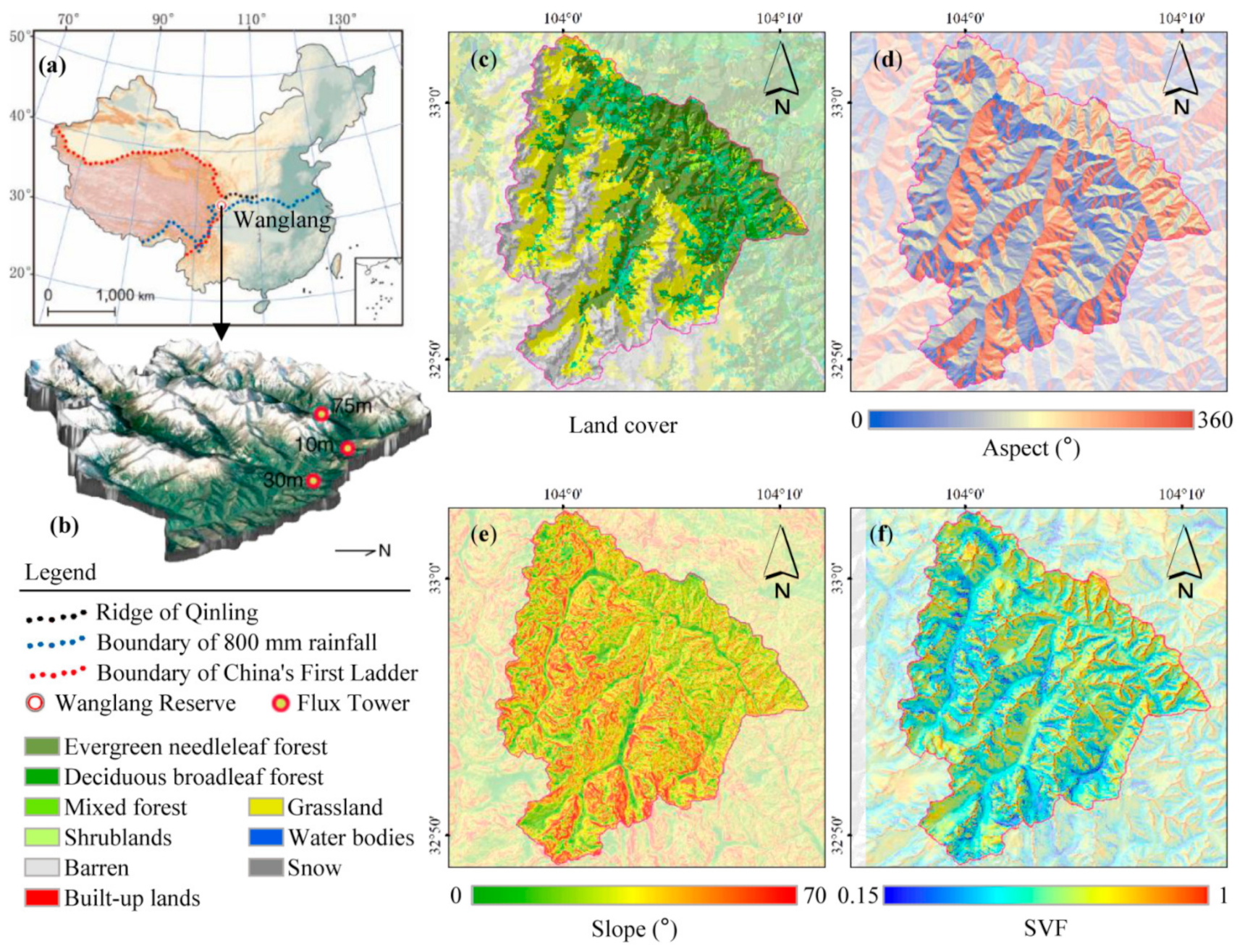
2.2.1. Study Area

As shown in Figure 1a, Wanglang National Nature Reserve (103°50′–104°58′E, 32°49′–33°02′N, referred to as Wanglang Reserve in the following) is located at the intersection of the 800 mm rainfall line, the boundary of China’s first Ladder, and the ridge of Qinling mountain, which is a typical mountainous region in southwest China. As shown in Figure 1c, the total area of the Wanglang Reserve is approximately 320 km², and includes evergreen needleleaf forest (ENF, 27.10%), deciduous broadleaf forest (DBF, 1.42%), mixed forest (MF, 11.85%), shrubland (SHR, 6.66%), grassland (GRA, 25.11%), and other lands (27.86%).

In 2017, an integrated observation and experiment station for mountain ecological remote sensing (referred to as Wanglang station in the following) was established in the Wanglang Reserve (Figure 1b). The main reasons for selecting the Wanglang Reserve to carry out research related to mountain ecological remote sensing are that (1) the topographic features of Wanglang Reserve are heterogeneous (Figure 1d–f), with elevation, slope, and SVF ranges of 1699–4914 m, 0–79°, and 0.15–1.00, respectively, and (2) the location of Wanglang Reserve is important for research associated with global climate change. Wanglang station mainly contains three observation systems (as shown in Supplementary Figure S1), including a shrubland tower with a height of 10 m, an MF tower with a height of 30 m, and an ENF tower with a height of 75 m.

As shown in Figure 2, during Day Of Year (DOY) 1–273 in 2020, the annual average air temperature, soil temperature, incoming solar radiation, precipitation, and VPD over Wanglang Reserve were 5.52 °C, 8.22 °C, 152.63 w m⁻², 639 mm, and 2.72 hpa, respectively. In general, the seasonal characteristics of Wanglang Reserve can be mainly described as (1) dry season (i.e., from November to April of the next year) with abundant sunshine, low rainfall, low air humidity, and low temperature, and (2) wet season (i.e., from May to October) with high-frequency cloudiness, concentrated heavy rainfall, high air humidity, and high temperature. Over Wanglang Reserve, the phenomenon that the simultaneous appearance of high heat, heavy rainfall, and significant diurnal temperature difference in the wet season, maximally promotes vegetation growth, and is conducive to the accumulation of vegetation biomass.

2.2.2. Data Processing

Due to the availability of time-series tower-based measurements, the study period of this work is from January to September 2020. As shown in

Table 1. Description of multiple datasets used in this study.

Dataset	Variable	Resolution	Reference
MCD15A2H a	LAI/FPAR	500 m/8-day	[69]
MOD13Q1 Version 6 a	NDVI/EVI	250 m/16-day	[70]
MOD11A2 Version 6 a	LST	1 km/8-day	[71]
Sentinel-2 Level-1C b	Surface albedo	10 m/10-day	[72]
Landsat-8 Level-1T c	Surface albedo	30 m/16-day	[73]
SRTM DEM	Elevation	30 m	[74]
Open Land Map	Soil properties	250 m	[75]

^a All available scenes between 1 January 2020, and 1 October 2020. ^b Four scenes obtained on 25 January 2019, 27 September 2019, 25 March 2020, and 3 June 2020. ^c One scene obtained on 1 July 2019.

, multiple datasets were used in this work. Besides tower-based measurements, all other data were prepared at 30 m resolution, including soil texture, LST (8-day), LAI (8-day), EVI (16-day), fraction of photosynthetically active radiation absorbed (FPAR, 8-day), land cover, and topographic features (i.e., elevation, aspect, slope, SVF, and watershed boundary). Soil texture maps at the 250 m resolution and MODIS LST at the 1 km resolution were resampled to 30 m resolution by assuming the soil type or LST of all the subpixels are the same as those of each coarse pixel.

• Tower-based data

Tower-based measurements were adopted in this work, including half-hour air temperature, incoming solar radiation, precipitation, and vapor pressure deficit (VPD). Daily data were calculated from these half-hour measurements to drive the GPP models. All tower-based data were processed according to Wutzler, Lucas-Moffat [76], with detailed information available at the online service (https://www.bgc-jena.mpg.de/bgi/index.php/Services/, accessed on 23 December 2020).

• Land cover map

In this study, a high-resolution land cover map was obtained from multi-temporal Sentinel-2 surface albedo data. Four Sentinel-2 surface albedo data with difference dates were used to provide seasonal information [77], which is useful for LC classification. The Level-1C products were firstly pre-processed by radiometric calibration and atmospheric correction (i.e., Sen2Cor). An object-oriented classification approach with a validation accuracy of ~89.68% [77], was then used to generate the 10-m land cover map from albedo information of the blue, green, red, and near-infrared bands. The main land cover types in the 10-m land cover map were evergreen needleleaf forest, deciduous broadleaf forest, mixed forest, shrubland, and grassland. To maintain consistency with the spatial resolution of other data, the 10-m land cover map was resampled to 30-m by assuming that the land cover type of each 30 m pixel was the dominant type (i.e., having the largest percentage of area) of all the 10-m subpixels.

• Time-series LAI, FPAR, and EVI maps

To ensure the reliability of MODIS LAI, FPAR, and EVI time-series data, those values with corresponding quality control (QC) values less than 64 (i.e., LAI and FPAR) or quality assurance (QA) values less than 1 (i.e., EVI) were selected, and missing values gap-filled using the linear interpolation method. In addition, the MODIS LAI, FPAR, and EVI time-series data were preprocessed with the Savitzky-Golay filter model (SG) due to noise.

The UofT LAI algorithm, developed from the four-scale geometrical optical model (FSGOM) [78], and the Spatial and Temporal Nonlocal Filter-Based Data Fusion Method (STNLFFM) [79] were adopted to generate high spatiotemporal resolution LAI maps. In this study, the UofT LAI algorithm was used to retrieve an LAI map at the 30 m resolution from the cloud-free Landsat-8 image, and then the STNLFFM was adopted to generate LAI maps at the resolutions of 30 m and 8-days from the 30-m LAI map and time-series MODIS LAI maps. Similar to the above generation of LAI maps, time-series EVI maps at 30 m resolution were also obtained from an EVI image from the Landsat-8 data and MODIS EVI data using SG and STNLFFM. Based on the method in [51], time-series FPAR maps at 30 m resolution were obtained by fusing an NDVI image from the Landsat-8 data and time-series MODIS FPAR data in conjunction with topographic features.

• Topographic maps

Several topographic maps, including elevation, slope, aspect, watershed boundary, and sky-view factor (SVF), were obtained from SRTM DEM. In the derivation of the watershed boundary map, the threshold value of flow-accumulation was set as 2500 to retain the 1 km² footprint area of the three observation towers. SVF was calculated using the method of Zaksek et al. (2011) [68]:

$$SVF=\frac{1}{n}{\displaystyle \sum _{i=1}^n\left(1-\sin h_i\right)}$$

(33)

where n and h_i are the number of directions and the vertical altitude angle, respectively. More descriptions about the calculation of SVF can be found in the online service (https://iaps.zrc-sazu.si/en/rvt#v, accessed on 1 December 2020).

2.3. Model Implementation

In this work, the MOD17, TL-LUE, MTL-LUE, TG, MTG, BEPS, and BTL models were all run at the spatial resolution of 30 m. As for the time resolution, MOD17, TL-LUE, MTL-LUE, BEPS, and BTL models were run at the daily step, whereas the time step of TG and MTG was 8-day. The main input data of these seven models are shown in

Table 2. Main input data of MOD17, TL-LUE, MTL-LUE, TG, MTG, BEPS, and BTL.

Model	Input Data
	Tower-Based (Daily)	Vegetation-Related (30 m)	Topography-Related (30 m)
MOD17	Rtotala, Tminb, VPDdaytimec	LC, LAI	-
TL-LUE	Rtotal, Tmin, VPDdaytime	LC, LAI	-
MTL-LUE	Rtotal, Tmin, VPDdaytime	LC, LAI	Elevation, slope, aspect, SVF
TG	-	LC, EVI, LST	-
MTG	-	LC, EVI, LST, FPAR	Elevation, slope, aspect
BEPS	Rtotal, Pred, Tmin, Tmaxe, Tavef	LC, LAI, soil type	-
BTL	Rtotal, Pre, Tmin, Tmax, Tave	LC, LAI, soil type	Elevation, slope, aspect, watershed

^a daily total incoming solar radiation; ^b daily minimum air temperature; ^c daytime average VPD; ^d daily total precipitation; ^e daily minimum air temperature; ^f daily average air temperature.

. In this work, the NEE measurements are not enough to build reliable models for tower-based GPP estimation [76,80]. Due to the unavailability of tower-based GPP, this work calibrated the model parameters of MOD17, TL-LUE, MTL-LUE, TG, MTG, BEPS, and BTL using reference values from previous studies (as shown in Supplementary Table S1). Zhou et al. (2016) [35] optimized the sensitive parameters of the TL-LUE and MOD17 models at global tower sites, which could provide reliable values of model parameters. Moreover, MTL-LUE has the same unknown parameters as the TL-LUE model. The different canopy albedo (i.e., α) values across vegetation types were set according to Wu et al. (2015) [37], and all other parameter values for MOD17, TL-LUE, and MTL-LUE in different vegetation types were obtained from Zhou et al. (2016) [35]. Xie and Li [23] optimized the sensitive parameters of TG (m_TG) and MTG (m_MTG) at 16 mountainous sites, and Dong et al. (2017) [81] calibrated the minimum, optimum, and maximum LST for vegetation photosynthesis at 155 tower sites. In this work, the parameter values of TG and MTG across vegetation types were obtained from Xie and Li [23] and Dong et al. (2017) [81]. Liu et al. (2018) [82] adopted BEPS to simulate carbon and water fluxes over China during 2003–2012, and their GPP estimates matched well with tower-based GPP at 38 sites. In this work, the key parameter values of BEPS across vegetation types were mainly obtained from Liu et al. (2018) [82] and He et al. (2019) [83]. In the BTL model, the biophysical parameters were set to the same values in BEPS, and the values of the hydrological parameters were set according to Govind et al. (2009) [18].

2.4. Model Comparison

In this work, MOD17, TL-LUE, MTL-LUE, BEPS, and BTL models were run at a daily time step, while TG and MTG were run at an 8-day time step. The annual GPP maps were summed from those daily (i.e., MOD17, TL-LUE, MTL-LUE, BEPS, and BTL) or 8-day maps of GPP estimates (i.e, TG and MTG). The multiple annual GPP maps from the seven models were then adopted for the model comparison. The relationships between multiple annual GPP maps and topographic maps (i.e., elevation, slope, aspect, and SVF) were also analyzed, to further illustrate the model responses to surface topography.

3. Results

3.1. Spatial Characteristics of Multiple Annual GPP Estimates

Spatial distributions of annual GPP estimates from the MOD17, TL-LUE, MTL-LUE, TG, MTG, BEPS, and BTL models over Wanglang Reserve are shown in Figure 3, and their statistics are presented in

Table 3. Mean (gC m⁻²yr⁻¹), standard deviation (SD, gC m⁻²yr⁻¹), and coefficient of variation (CV, %) values of multiple annual GPP estimates in forest, shrub, grass, and all pixels.

Model	Forest			Shrub			Grass			All
	Mean	SD	CV	Mean	SD	CV	Mean	SD	CV	Mean	SD	CV
MOD17	1431	152	11	1006	143	14	1457	341	23	1401	267	19
TL-LUE	1021	116	11	829	134	16	1123	278	25	1039	207	20
MTL-LUE	1148	208	18	713	168	23	1006	306	30	1059	276	26
TG	527	192	36	218	153	71	159	177	112	370	255	69
MTG	411	192	47	295	235	80	110	139	126	296	228	77
BEPS	663	169	25	707	143	20	756	177	23	699	175	25
BTL	901	443	49	871	412	47	1088	463	43	963	457	47

. In general, multiple annual GPP estimates from the seven models over Wanglang Reserve showed similar spatial distributions. As for the three LUE models, the annual GPP estimates from the MTL-LUE model had a higher spatial variation (CV = 26%) than those from TL-LUE (CV = 20%) and MOD17 (CV = 19%) for all pixels. The annual GPP estimates from MTG and BTL models also presented a higher spatial variation than those from TG and BEPS, with CV values increased by 8% and 22%, respectively.

At the watershed scale, GPP estimates from the seven models presented different annual values. The GPP estimates from MTL-LUE had a lower annual value than those from the MOD17 model for the forest, shrub, and grass pixels, with the mean value decreasing by 283, 293, and 451 gC m⁻²yr⁻¹, respectively. Compared to the TL-LUE model, the GPP estimates from MTL-LUE had a higher annual value for forest pixels (increasing mean value by 127 gC m⁻²yr⁻¹), but a lower annual value in for shrub pixels (decreasing mean value by 116 gC m⁻²yr⁻¹) and grass pixels (decreasing mean value by 117 gC m⁻²yr⁻¹). Compared to the TG model, the GPP estimates from MTG had a higher annual value for shrub pixels (increasing mean value by 77 gC m⁻²yr⁻¹), but a lower annual value for forest pixels (decreasing mean value by 116 gC m⁻²yr⁻¹) and grass pixels (decreasing mean value by 49 gC m⁻²yr⁻¹). The GPP estimates from BTL had a higher annual value than those from the BEPS model for the forest, shrub, and grass pixels, with the mean value increasing by 238, 164, and 332 gC m⁻²yr⁻¹, respectively.

3.2. Comparisons among Multiple Annual GPP Estimates

As shown in Figure 4, the relationships between annual GPP_MTL-LUE and GPP_MOD17 (R² = 0.77, RMSE = 368 gC m⁻²yr⁻¹, rRMSE = 35%), GPP_MTL-LUE and GPP_TL-LUE (R² = 0.65, RMSE = 165 gC m⁻²yr⁻¹, rRMSE = 16%), and GPP_MTG and GPP_TG (R² = 0.78, RMSE = 141 gC m⁻²yr⁻¹, rRMSE = 48%) were all closer than that between annual GPP_BEPS and GPP_BTL (R² = 0.33, RMSE = 465 gC m⁻²yr⁻¹, rRMSE = 48%)_. The GPP_MOD17 of almost all the pixels had a higher annual value than the GPP_MTL-LUE, and the GPP_TL-LUE of most pixels also had a higher annual value than the GPP_MTL-LUE. The difference between annual GPP_MTL-LUE and GPP_MOD17 in forest pixels was lower than that in shrub and grass pixels, with the rRMSE decreasing by 16% and 19%, respectively. The rRMSE between annual GPP_MTL-LUE and GPP_TL-LUE presented a similar value in the forest (15%), shrub (18%), and grass (16%) pixels. The GPP_TG of most forest and grass pixels had a higher annual value than the GPP_MTG, whereas the GPP_TG of most shrub pixels had a lower annual value than the GPP_MTG. Although the rRMSE between annual GPP_BEPS and GPP_BTL showed a similar value in the forest (47%), shrub (44%), and grass (50%) pixels, the R² between annual GPP_BEPS and GPP_BTL in forest pixels was higher than that in shrub and grass pixels by 0.13 and 0.33, respectively. The GPP_BEPS of most forest and grass pixels presented a lower annual value than the GPP_BTL.

As shown in Figure 5, the relationships between annual GPP_BTL and GPP_MTL-LUE (R² = 0.29, RMSE = 399 gC m⁻²yr⁻¹), and GPP_MTL-LUE and GPP_MTG (R² = 0.34, RMSE = 798 gC m⁻²yr⁻¹) were closer than that between annual GPP_BTL and GPP_MTG (R² = 0.02, RMSE = 821 gC m⁻²yr⁻¹)_. The GPP_MTG of almost all pixels had a higher annual value than the GPP_BTL and the GPP_MTL-LUE, and the GPP_MTG of the most pixels was similar to GPP_BTL. The difference between annual GPP_BTL and GPP_MTL-LUE in grass pixels was lower than that in shrub and forest pixels, with rRMSE decreased by 11% and 17%, respectively. Forest and shrub pixels showed a lower rRMSE value between annual GPP_MTL-LUE and GPP_MTG than grass pixels by 23% and 22%, respectively. Forest and shrub pixels showed a lower rRMSE value between annual GPP_MTL-LUE and GPP_MTG than grass pixels by 23% and 22%. The difference between annual GPP_BTL and GPP_MTL-LUE in grass pixels was also larger than that in shrub and forest pixels, with rRMSE decreased by 31% and 26%, respectively.

3.3. Relationships between Annual GPP Estimates and Topographical Factors

As shown in Figure 6a,e,i,m, the ratio between GPP_MTL-LUE and GPP_MOD17 showed similar relationships with topographical factors in forest, shrub, and grass pixels, which can be mainly summarized as (1) decreasing with an increase in elevation or slope, (2) increasing with an increase in SVF, and (3) presenting no apparent relationship with aspect. More specifically, a slight decrease was observed in the ratio between GPP_MTL-LUE and GPP_MOD17 when the slope varied from 0° to 40°, and then the ratio decreased rapidly in the slope range of 40°–80°. The ratio between GPP_MTL-LUE and GPP_MOD17 decreased when the elevation varied from 2500 m to 3500 m, whereas it showed no obvious variation in the elevation range of 3500–4500 m.

As shown in Figure 6b,f,j,n, the ratio between GPP_MTL-LUE and GPP_TL-LUE in forest pixels presented a higher value than that in shrub and grass pixels, and its relationships with topographical factors were similar in the forest, shrub, and grass pixels. The ratio between GPP_MTL-LUE and GPP_TL-LUE decreased with elevation increasing or SVF decreasing, and no obvious relationship was found with aspect. A slight decrease was also observed in the ratio between GPP_MTL-LUE and GPP_TL-LUE when the slope varied from 0° to 40°, and then the ratio decreased rapidly in the slope range of 40°–80°.

As shown in Figure 6c,g,k,o, the ratio between GPP_MTG and GPP_TG in shrub pixels presented a higher value than that in forest and grass pixels, and showed similar relationships with topographical factors in forest, shrub, and grass pixels. In general, the ratio between GPP_MTG and GPP_TG (1) decreased with increasing slope or decreasing SVF, (2) increased gradually and then decreased with the aspect varying from 0° to 360°, and (3) decreased gradually when the elevation varied from 2500 m to 3500 m, and then increased when the elevation varied from 3500 m to 4000 m.

As shown in Figure 6d,h,l,p, the ratio between GPP_BTL and GPP_BEPS presented similar relationships with topographical factors in forest, shrub, and grass pixels, which can be mainly summarized as (1) decreasing rapidly with increasing elevation, (2) increasing gradually with increasing slope, (3) decreasing and then increasing with the aspect varying from 0° to 360°, and (4) increasing gradually with increasing SVF.

4. Discussion

4.1. Improvements of MTL-LUE, MTG, and BTL in Simulating GPP over Mountainous Areas

LUE models, VI-based models, and process-based models are the three main approaches for spatial-continuous GPP estimation, such as the MOD17, TL-LUE, TG, and BEPS models. However, most of these three GPP models overlook the effect of topography on the vegetation photosynthesis process, and treat the terrestrial surface as flat areas. Over the last decade, Xie and Li [22], Xie and Li [23], and Govind et al. (2009) [18] have proposed a mountain LUE model (i.e., MTL-LUE), a mountain VI-based model (i.e., MTG), and a mountain process-based model (i.e., BTL) to improve the GPP estimation over mountain areas. The GPP estimates from these three mountain GPP models have been proved to better match tower-based GPP than those from the original models (i.e., TL-LUE, TG, and BEPS) at the site scale.

In this study, three LUE models (i.e., MOD17, TL-LUE, and MTL-LUE), two VI-based models (i.e., TG and MTG), and two process-based models (i.e., BEPS and BTL) were adopted to obtain GPP estimates for a mountainous watershed (i.e., Wanglang Reserve). Results showed that multiple annual GPP estimates from different models presented a similar spatial distribution over Wanglang Reserve. The annual GPP estimates from mountain GPP models were found to have a higher spatial variation than those from the original models, highlighting that incorporating topographic information into GPP models might improve the understanding of the high spatial heterogeneity of the vegetation photosynthesis process over mountainous areas.

4.1.1. Improvement of MTL-LUE over MOD17 and TL-LUE

MOD17 is a big-leaf LUE model with the assumption that the whole canopy can absorb direct and diffuse solar radiation simultaneously. Various studies suggested that sunlit leaves, which absorb both direct and diffuse radiation, are easily light-saturated, and the photosynthetic capacity of shaded leaves, which only absorb diffuse radiation, is normally constrained by low APAR [10,29,30,31]. TL-LUE and MTL-LUE are both two-leaf LUE models with different treatments of sunlit and shaded leaves. In the TL-LUE model, an empirical relationship established from the diffuse and total incoming radiation measurements at four sites [29], is adopted to separate the direct and diffuse radiation from the total radiation [33,35]. This empirical relationship may cause biased separation of direct and diffuse radiation over mountainous areas because (1) the direct radiation is affected by local solar zenith angle (which can be expressed by slope and aspect) [38,84] and (2) the diffuse radiation would reduce when the hemispherical sky dome is partially blocked (can be expressed by SVF) [38,40,85]. Moreover, TL-LUE also neglects the effect of topography on the portion of sunlit and shaded canopy areas, which may lead to bias in the separation of sunlit and shaded LAI, because the sunlit canopy area can be altered by the relative positioning of geotropic trees [43,44,45]. The MTL-LUE model incorporates topographic attributes (i.e., slope, aspect, and SVF) into the TL-LUE model to improve the characterization of direct and diffuse radiation (as shown in Figure 7a) and the separation of sunlit and shaded LAI (as shown in Figure 7b).

At the watershed scale, the GPP estimates from MTL-LUE were found to have a lower annual value than those from MOD17 in all the forest, shrub, and grass pixels, with the mean value decreasing by 127 gC m⁻²yr⁻¹. The lower annual GPP estimates from MTL-LUE may stem from the fact that the MTL-LUE model considers the decrease of incoming solar radiation caused by the shielding of topography: (1) direct radiation varies with the geometric relationship between the tilt of ground surface and the solar position and (2) diffuse radiation decreases with the tilt of the ground surface itself and surrounding terrain. Results also indicated that the GPP estimates from MTL-LUE were observed to have a similar value with those from TL-LUE. Over mountainous areas, the difference between GPP estimates from MTL-LUE and TL-LUE at the watershed scale depends on the gap between the GPP variations of sunlit and shaded leaves: (1) the sunlit GPP estimates from MTL-LUE would be higher in the sunlit terrain (due to the higher sunlit LAI and direct radiation) and lower in the shaded terrain (due to the lower sunlit LAI and direct radiation) than those from TL-LUE and (2) the shaded GPP estimates from MTL-LUE would be lower in the sunlit terrain (due to the lower shaded LAI and lower diffuse radiation) and higher in the shaded terrain (due to the higher shaded LAI) than those from TL-LUE.

Our finding that the ratio between annual GPP estimates from MTL-LUE and MOD17 (or TL-LUE) decreased with increasing slope or decreasing SVF, is expected because more heterogeneous terrain (e.g., a higher slope and a lower SVF) would cause a greater decrease in received solar radiation. When the elevation varied from 2500 m to 3500 m, although the diffuse radiation increased due to the increase of SVF (as shown in Figure 8), direct radiation would decrease because of the increased slope, which may be the reason for the decrease in the ratio between annual GPP estimates from MTL-LUE and MOD17 (or TL-LUE).

4.1.2. Improvement of MTG over TG

TG is a VI-based model which uses the combination of EVI and LST to obtain GPP estimates [12]. In the model application, the LST input of TG is always provided by MODIS products at coarse spatial resolutions, which may lose a large portion of topographic characteristics over mountainous areas [51]. The MTG model incorporates an elevation-corrected factor and a radiation-corrected factor into the TG model to address the effect of elevation on temperature [52,53] and characterize the contribution of the incoming solar radiation to the spatial variation in temperature [52,54], respectively.

At the watershed scale, the GPP estimates from MTG had a higher annual value than those from TG in shrub pixels, while they presented a lower annual value than those from TG in forest pixels and grass pixels. As for the effect of elevation on temperature, higher GPP estimates from MTG can occur in situations when (1) the elevation is low and the LST is smaller than the optimum photosynthesis temperature and (2) the elevation is high and the LST is higher than the optimum photosynthesis temperature. Lower GPP estimates from MTG can occur in situations when (1) the elevation is low and LST is greater than the optimum photosynthesis temperature and (2) the elevation is high and LST is lower than the optimum photosynthesis temperature. As for the contribution of the incoming solar radiation to the spatial variation in temperature, higher incoming solar radiation would lead to a higher GPP estimate from MTG.

Results also indicated that the ratio between annual GPP estimates from MTG and TG decreased with increasing slope or decreasing SVF, possibly because a higher slope and a lower SVF would lead to lower incoming solar radiation. The ratio between annual GPP estimates from MTG and TG was observed to decrease and then increase with elevation varying from 2500 m to 4000 m, as incoming solar radiation decreased and increased due to the increase of slope in the elevation range of 2500 m to 3500 m, and the decrease of slope in the elevation range of 3500 m to 4000 m over Wanglang Reserve, respectively. The finding in this study that the ratio between annual GPP estimates from MTG and TG increased gradually and then decreased with aspects varying from 0° to 360° may be caused by the high incoming solar radiation in the sunlit terrain and low incoming solar radiation in the shaded terrain during the growing season.

4.1.3. Improvement of BTL over BEPS

BEPS is a two-leaf process-based model using biological, climatic, and soil variables to characterize the vegetation photosynthesis process [29,34], which has been adopted as an effective tool to simulate the carbon and water fluxes over the globe [66,67]. In the BEPS model, each pixel is assigned the same value of radiation and temperature. BTL is an eco-hydrological model that integrates BEPS with a spatially distributed hydrological model, which was designed to obtain accurate estimations of the carbon and water fluxes over mountainous areas [18]. BTL improves the GPP estimation from BEPS over mountainous areas mainly through adding: (1) the effect of elevation on temperature, i.e., lower temperatures in pixels at higher elevation in the watershed than those at lower elevations [52,53], (2) spatial heterogeneity of incoming solar radiation, i.e., shaded terrain always receives less radiation than the sunlit terrain [38,39,40,41,86], and (3) the movement of soil water, by assuming that each pixel is connected to its surrounding 8 pixels, i.e., soil water of pixels with a higher elevation in the watershed could move to pixels with a lower elevation (as shown in Figure 7c) [18,20,87].

Results showed that the GPP estimates from BTL had a higher annual value than those from the BEPS model for the forest, shrub, and grass pixels, with the mean value increasing by 264 gC m⁻²yr⁻¹. Over mountainous areas, the difference between GPP estimates from BTL and BEPS at the watershed scale depended on the combined spatial effect of various environmental indicators on the vegetation photosynthesis process. The capacity of vegetation photosynthesis was not directly associated with incoming solar radiation, temperature, or soil water. For example, when considering the single effect of incoming solar radiation on GPP, if the incoming solar radiation itself is high, a further increase in radiation would only result in a subtle GPP increase due to light saturation [29]. However, higher radiation would increase evapotranspiration and decrease soil water, and thus the GPP would decrease. Therefore, at higher radiation, GPP variability depends on the gap between the GPP increase (resulting from higher radiation) and the GPP decrease (resulting from lower soil water). The ratio between annual GPP estimates from BTL and BEPS was found to increase as SVF and elevation increased, and as slope decreased, possibly due to a higher SVF leading to higher incoming solar radiation, and a lower slope leading to increased soil water [20]. The lower ratio between annual GPP estimates from BTL and BEPS was observed in the aspect range of 90°–110°, with the possible reason being that the radiation in this aspect range is most suitable for vegetation photosynthesis (i.e., GPP increased a lot by high radiation and decreased little by lower soil water).

4.2. Comparisons of GPP Estimates from MTL-LUE, MTG, and BTL

To improve GPP estimation over mountainous areas, we propose the use of MTL-LUE, MTG, and BTL by incorporating topographic characteristics into the LUE, VI-based, and process-based models. Their improvement at site scale (more closely aligning with tower-based GPP) has been proved in previous studies [18,22,23], and their improvement at the watershed scale has also been illustrated in the above section. Besides discussing the improvement of these three mountain GPP models at the watershed scale, one of the other objectives of this work was to compare the GPP estimates from MTL-LUE, MTG, and BTL over mountainous watersheds. Results showed that the relationships between annual GPP estimates from BTL and MTL-LUE (R² = 0.29, RMSE = 399 gC m⁻²yr⁻¹) and MTL-LUE and MTG (R² = 0.34, RMSE = 798 gC m⁻²yr⁻¹) were closer than that between BTL and MTG (R² = 0.02, RMSE = 821 gC m⁻²yr⁻¹)_. In general, the discrepancy of annual GPP estimates among MTL-LUE, MTG, and BTL might result from model parameters and structure.

The GPP discrepancies of these models may stem from differently calibrated values of sensitive parameters, such as the maximum LUE in MTL-LUE [35,88], the slope between GPP and the combination of temperature and greenness in MTG [12,46,50], and the maximum carboxylation rate in BTL [89,90]. The sensitive parameters in MTL-LUE, MTG, and BTL are different, and their ecological definitions are also different. One solution is to calibrate these sensitive model parameters with tower-based GPP data, thus increasing the uniformity of the GPP estimates from these three different models. In this work, the NEE measurements were not enough to build reliable models for tower-based GPP estimation [76,80]. As shown in Figure 9, a standardized index for annual GPP estimates was used to address the discrepancies caused by model parameters. The standardized index of multiple annual GPP estimates was observed to present a similar spatial distribution over Wanglang Reserve, suggesting that the calibration of model parameters in different models is important for GPP estimation over mountainous areas. Further work should be carried out to obtain more reference values of the sensitive model parameters across vegetation types as there are more mountainous observations.

Different model structures adopted in MTL-LUE, MTG, and BTL may be another source for the GPP discrepancies. MTL-LUE is developed from radiation conversion efficiency, mainly assuming that (1) GPP is directly related to the APAR and actual LUE [24], (2) sunlit leaves can absorb both direct and diffuse radiation whereas shaded leaves only absorb diffuse radiation [10,29,30,31], (3) direct radiation varies with the geometric relationship between the tilt of ground surface and the solar position [38,84] and diffuse radiation decreases by the tilt of the ground surface itself and surrounding terrain [38,40,85], and (4) the portion of sunlit and shaded canopy areas is affected by the relative positioning of geotropic trees [43,44,45]. The main assumptions in the MTG model are that (1) EVI can effectively describe water stress, because vegetation suffering from drought always senesces or partially loses foliage to conserve water [12,91,92], (2) LST can well characterize the summer drought stress and the photosynthetic inactivation for strongly evergreen vegetation, because the representative characteristics of the summer drought periods and the inactive photosynthetic periods are high temperature [93] and low temperature [12], (3) the temperature tends to decrease with as elevation increases, and (4) incoming solar radiation (only including the direct radiation) varies with the geometric relationship between the tilt of the ground surface and the solar position [38,84] and a higher incoming solar radiation would lead to a higher temperature [52,54]. BTL is an eco-hydrological model which assumes that (1) the capacity of vegetation photosynthesis is associated with various environmental indicators (i.e., temperature, radiation, and soil water) and ecological processes (i.e., evapotranspiration), (2) sunlit leaves can absorb both direct and diffuse radiation whereas shaded leaves only absorb diffuse radiation [10,29,30,31], (3) topography has a redistributing effect on the spatial distribution of incoming solar radiation [38,39,40,41,86] and temperature [52,53], and (4) soil water of pixels with a higher elevation in the watershed could move to pixels with a lower elevation [18,20,87].

MTL-LUE, MTG, and BTL are developed from the model structure of TL-LUE/MOD17, TG, and BEPS, respectively. Besides these above assumptions associated with topography, all others are the original assumptions in MOD17, TL-LUE, TG, and BEPS. As shown in Figure 10, the discrepancy of annual GPP estimates among MOD17, TL-LUE, TG, and BEPS, was also observed, suggesting that the GPP discrepancy over mountainous areas may be caused by the different original model structures used in MOD17, TL-LUE, TG, and BEPS. Moreover, the modeling strategies used to describe the complex effect of topography on the vegetation photosynthesis process are also different in MTL-LUE, MTG, and BTL.

4.3. The Existing Limitations and Future Prospects

Currently, obtaining accurate leaf-sun angle values is difficult, especially over mountainous areas. Most GPP models assume the mean leaf-sun angle as a constant, which might create uncertainties in the final GPP estimates. Our future work would try to find improvements in GPP estimation with the use of more accurate leaf-sun angle values in the carbon modeling process. In this work, several topographic maps were obtained from the 30 m SRTM DEM, and it should be noted that any uncertainties in the original DEM data could lead to bias in the results. Besides the surface topography, vegetation heterogeneity (LAI and LC) is also important in GPP estimation [94]. Over mountainous areas, LAI and LC maps have been reported to present high uncertainties because of the high levels of cloud, aerosol, and snow in remote sensing observations [95,96]. Future work should develop reliable algorithms to obtain reliable LAI and LC maps at fine resolutions.

5. Summary

LUE models, VI-based models, and process-based models are the three main approaches for spatial-continuous GPP estimation. In this work, three LUE models (i.e., MOD17, TL-LUE, and MTL-LUE), two VI-based models (i.e., TG and MTG), and two process-based models (i.e., BEPS and BTL) were adopted to obtain GPP estimates for a mountainous watershed (i.e., Wanglang Reserve). At the watershed scale, the annual GPP estimates from MTL-LUE, MTG, and BTL were found to have higher spatial variation than those from the original models (increasing the spatial coefficient of variation by 6%, 8%, and 22%), highlighting that incorporating topographic information into GPP models might improve understanding of the high spatial heterogeneity of the vegetation photosynthesis process over mountainous areas. Obvious discrepancies were also observed in the GPP estimates from MTL-LUE, MTG, and BTL, with determination coefficients ranging from 0.02–0.29 and root mean square errors ranging from 399–821 gC m⁻²yr⁻¹. Our study highlights the importance of considering surface topography when modeling GPP over mountainous areas, and suggests that more attention should be given to the discrepancies in GPP estimates from different models.

The BTL model considers the combined spatial effect of various environmental indicators and ecological processes on the vegetation photosynthesis process. The limitation of BTL over large areas is that it’s complicated model structure requires a large number of input data and ecological parameters. MTL-LUE only considers the process of radiation conversion, and it also requires meteorological data as input. Although the understanding of the vegetation photosynthesis process in MTG is not as detailed as that in BTL and MTL-LUE, the MTG model takes advantage of extensive remotely sensed data and topographical information (i.e., estimating GPP without ground data), and can also be used to obtain mountain GPP over large areas. Based on the results over Wanglang Reserve, the following strategies are suggested for GPP estimation over large-scale mountainous areas: (1) if relevant ecological parameters and meteorological data are sufficient and reliable, the BTL model is the best choice, (2) if only reliable meteorological data are available in the study area, the MTL-LUE model is more suitable than BTL and MTG, and (3) if there is no reliable ground data in the study area, the MTG model can be used as the simulation tool.

References

1. Sellers, P.J.; Schimel, D.S.; Moore, B.; Liu, J.; Eldering, A. Observing carbon cycle–climate feedbacks from space. Proc. Natl. Acad. Sci. USA 2018, 115, 7860–7868. [Google Scholar] [CrossRef] [PubMed] [Green Version]
2. Beer, C.; Reichstein, M.; Tomelleri, E.; Ciais, P.; Jung, M.; Carvalhais, N.; Rödenbeck, C.; Arain, M.A.; Baldocchi, D.; Bonan, G.B.; et al. Terrestrial gross carbon dioxide uptake: Global distribution and covariation with climate. Science 2010, 329, 834–838. [Google Scholar] [CrossRef] [PubMed] [Green Version]
3. Seddon, A.W.R.; Macias-Fauria, M.; Long, P.R.; Benz, D.; Willis, K.J. Sensitivity of global terrestrial ecosystems to climate variability. Nature 2016, 531, 229–232. [Google Scholar] [CrossRef] [PubMed] [Green Version]
4. Piao, S.; Sitch, S.; Ciais, P.; Friedlingstein, P.; Peylin, P.; Wang, X.; Ahlström, A.; Anav, A.; Canadell, J.; Cong, N.; et al. Evaluation of terrestrial carbon cycle models for their response to climate variability and to CO2trends. Glob. Chang. Biol. 2013, 19, 2117–2132. [Google Scholar] [CrossRef] [PubMed] [Green Version]
5. Kljun, N.; Calanca, P.; Rotach, M.W.; Schmid, H.P. A simple two-dimensional parameterisation for Flux Footprint Prediction (FFP). Geosci. Model Dev. 2015, 8, 3695–3713. [Google Scholar] [CrossRef] [Green Version]
6. Pan, L.; Xia, H.; Yang, J.; Niu, W.; Wang, R.; Song, H.; Guo, Y.; Qin, Y. Mapping cropping intensity in Huaihe basin using phe-nology algorithm, all Sentinel-2 and Landsat images in google earth engine. Int. J. Appl. Earth Obs. Geoinf. 2021, 102, 102376. [Google Scholar] [CrossRef]
7. Xiao, J.; Chevallier, F.; Gomez, C.; Guanter, L.; Hicke, J.A.; Huete, A.R.; Ichii, K.; Ni, W.; Pang, Y.; Rahman, A.F.; et al. Remote sensing of the terrestrial carbon cycle: A review of advances over 50 years. Remote Sens. Environ. 2019, 233, 111383. [Google Scholar] [CrossRef]
8. Running, S.W.; Nemani, R.R.; Heinsch, F.A.; Zhao, M.; Reeves, M.; Hashimoto, H. A Continuous Satellite-Derived Measure of Global Terrestrial Primary Production. Bioscience 2004, 54, 547–560. [Google Scholar]
9. Yuan, W.; Liu, S.; Zhou, G.; Zhou, G.; Tieszen, L.L.; Baldocchi, D.; Bernhofer, C.; Gholz, H.; Goldstein, A.; Goulden, M.; et al. Deriving a light use efficiency model from eddy covariance flux data for predicting daily gross primary production across biomes. Agric. For. Meteorol. 2007, 143, 189–207. [Google Scholar] [CrossRef] [Green Version]
10. Yan, H.; Wang, S.-Q.; Yu, K.-L.; Wang, B.; Yu, Q.; Bohrer, G.; Billesbach, D.; Bracho, R.; Rahman, F.; Shugart, H.H. A Novel Diffuse Fraction-Based Two-Leaf Light Use Efficiency Model: An Application Quantifying Photosynthetic Seasonality across 20 AmeriFlux Flux Tower Sites. J. Adv. Model. Earth Syst. 2017, 9, 2317–2332. [Google Scholar] [CrossRef] [Green Version]
11. Wu, C.; Niu, Z.; Gao, S. Gross primary production estimation from MODIS data with vegetation index and photosynthetically active radiation in maize. J. Geophys. Res. Space Phys. 2010, 115, 115. [Google Scholar] [CrossRef] [Green Version]
12. Sims, D.A.; Rahman, A.F.; Cordova, V.D.; Elmasri, B.Z.; Baldocchi, D.D.; Bolstad, P.V.; Flanagan, L.B.; Goldstein, A.H.; Hollinger, D.Y.; Misson, L.; et al. A new model of gross primary productivity for North American ecosystems based solely on the enhanced vegetation index and land surface temperature from MODIS. Remote Sens. Environ. 2008, 112, 1633–1646. [Google Scholar] [CrossRef]
13. Bonan, G.B. The Land Surface Climatology of the NCAR Land Surface Model Coupled to the NCAR Community Climate Model*. J. Clim. 1998, 11, 1307–1326. [Google Scholar] [CrossRef]
14. Immerzeel, W.W.; Petersen, L.; Ragettli, S.; Pellicciotti, F. The importance of observed gradients of air temperature and precip-itation for modeling runoff from a glacierized watershed in the Nepalese Himalayas. Water Resour. Res. 2014, 50, 2212–2226. [Google Scholar] [CrossRef] [Green Version]
15. Mizukami, N.; Clark, M.P.; Slater, A.; Brekke, L.D.; Elsner, M.M.; Arnold, J.R.; Gangopadhyay, S. Hydrologic Implications of Different Large-Scale Meteorological Model Forcing Datasets in Mountainous Regions. J. Hydrometeorol. 2014, 15, 474–488. [Google Scholar] [CrossRef]
16. Xia, H.; Qin, Y.; Feng, G.; Meng, Q.; Cui, Y.; Song, H.; Ouyang, Y.; Liu, G. Forest Phenology Dynamics to Climate Change and Topography in a Geographic and Climate Transition Zone: The Qinling Mountains in Central China. Forests 2019, 10, 1007. [Google Scholar] [CrossRef] [Green Version]
17. Qiu, Y.; Fu, B.; Wang, J.; Chen, L. Soil moisture variation in relation to topography and land use in a hillslope catchment of the Loess Plateau, China. J. Hydrol. 2001, 240, 243–263. [Google Scholar] [CrossRef]
18. Govind, A.; Chen, J.M.; Margolis, H.; Ju, W.; Sonnentag, O.; Giasson, M.-A. A spatially explicit hydro-ecological modeling framework (BEPS-TerrainLab V2.0): Model description and test in a boreal ecosystem in Eastern North America. J. Hydrol. 2009, 367, 200–216. [Google Scholar] [CrossRef]
19. Sabetraftar, K.; Mackey, B.; Croke, B. Sensitivity of modelled gross primary productivity to topographic effects on surface radiation: A case study in the Cotter River Catchment, Australia. Ecol. Model. 2011, 222, 795–803. [Google Scholar] [CrossRef]
20. Chen, J.M.; Chen, X.; Ju, W. Effects of vegetation heterogeneity and surface topography on spatial scaling of net primary productivity. Biogeosciences 2013, 10, 4879–4896. [Google Scholar] [CrossRef] [Green Version]
21. Guan, X.; Shen, H.; Li, X.; Gan, W.; Zhang, L. Climate Control on Net Primary Productivity in the Complicated Mountainous Area: A Case Study of Yunnan, China. IEEE J. Sel. Top. Appl. Earth Obs. Remote Sens. 2018, 11, 4637–4648. [Google Scholar] [CrossRef]
22. Xie, X.; Li, A. An Adjusted Two-Leaf Light Use Efficiency Model for Improving GPP Simulations Over Mountainous Areas. J. Geophys. Res. Atmos. 2020, 125, e2019JD031702. [Google Scholar]
23. Xie, X.; Li, A. Development of a topographic-corrected temperature and greenness model (TG) for improving GPP estimation over mountainous areas. Agric. For. Meteorol. 2020, 295, 108193. [Google Scholar] [CrossRef]
24. Monteith, J.L. Solar Radiation and Productivity in Tropical Ecosystems. J. Appl. Ecol. 1972, 9, 747–766. [Google Scholar] [CrossRef] [Green Version]
25. Running, S.; Mu, Q.; Zhao, M. MOD17A2H MODIS/terra Gross Primary Productivity 8-day L4 Global 500m SIN Grid, Version V006; NASA EOSDIS Land Processes DAAC: Sioux Falls, SD, USA, 2015.
26. Yuan, W.; Liu, S.; Yu, G.; Bonnefond, J.-M.; Chen, J.; Davis, K.; Desai, A.R.; Goldstein, A.; Gianelle, D.; Rossi, F.; et al. Global estimates of evapotranspiration and gross primary production based on MODIS and global meteorology data. Remote Sens. Environ. 2010, 114, 1416–1431. [Google Scholar] [CrossRef] [Green Version]
27. Zhang, Y.; Xiao, X.; Wu, X.; Zhou, S.; Zhang, G.; Qin, Y.; Dong, J. Data Descriptor: A global moderate resolution dataset of gross primary production of vegetation for 2000–2016. Sci. Data 2017, 4, 1–13. [Google Scholar] [CrossRef] [PubMed] [Green Version]
28. Xiao, X.; Hollinger, D.; Aber, J.; Goltz, M.; Davidson, E.; Zhang, Q.; Moore, B. Satellite-based modeling of gross primary production in an evergreen needleleaf forest. Remote Sens. Environ. 2004, 89, 519–534. [Google Scholar] [CrossRef]
29. Chen, J.; Liu, J.; Cihlar, J.; Goulden, M. Daily canopy photosynthesis model through temporal and spatial scaling for remote sensing applications. Ecol. Model. 1999, 124, 99–119. [Google Scholar] [CrossRef] [Green Version]
30. Roderick, M.L.; Farquhar, G.D.; Berry, S.L.; Noble, I.R. On the direct effect of clouds and atmospheric particles on the productivity and structure of vegetation. Oecologia 2001, 129, 21–30. [Google Scholar] [CrossRef] [PubMed]
31. Alton, P.B.; Ellis, R.; Los, S.; North, P. Improved global simulations of gross primary product based on a separate and explicit treatment of diffuse and direct sunlight. J. Geophys. Res. Space Phys. 2007, 112, 12. [Google Scholar] [CrossRef] [Green Version]
32. Guan, X.; Chen, J.M.; Shen, H.; Xie, X. A modified two-leaf light use efficiency model for improving the simulation of GPP using a radiation scalar. Agric. For. Meteorol. 2021, 307, 108546. [Google Scholar] [CrossRef]
33. He, M.; Ju, W.; Zhou, Y.; Chen, J.; He, H.; Wang, S.; Wang, H.; Guan, D.; Yan, J.; Li, Y.; et al. Development of a two-leaf light use efficiency model for improving the calculation of terrestrial gross primary productivity. Agric. For. Meteorol. 2013, 173, 28–39. [Google Scholar] [CrossRef]
34. Liu, J.; Chen, J.M.; Cihlar, J.; Park, W.M. A process-based boreal ecosystem productivity simulator using remote sensing inputs. Remote Sens. Environ. 1997, 62, 158–175. [Google Scholar] [CrossRef]
35. Zhou, Y.; Wu, X.; Ju, W.; Chen, J.M.; Wang, S.; Wang, H.; Yuan, W.; Black, T.A.; Jassal, R.; Ibrom, A.; et al. Global parameterization and validation of a two-leaf light use efficiency model for predicting gross primary production across FLUXNET sites. J. Geophys. Res. Biogeosci. 2016, 121, 1045–1072. [Google Scholar] [CrossRef]
36. Zan, M.; Zhou, Y.; Ju, W.; Zhang, Y.; Zhang, L.; Liu, Y. Performance of a two-leaf light use efficiency model for mapping gross primary productivity against remotely sensed sun-induced chlorophyll fluorescence data. Sci. Total. Environ. 2018, 613, 977–989. [Google Scholar] [CrossRef]
37. Wu, X.; Ju, W.; Zhou, Y.; He, M.; Law, B.E.; Black, T.A.; Margolis, H.A.; Cescatti, A.; Gu, L.; Montagnani, L.; et al. Performance of Linear and Nonlinear Two-Leaf Light Use Efficiency Models at Different Temporal Scales. Remote Sens. 2015, 7, 2238–2278. [Google Scholar] [CrossRef] [Green Version]
38. Huang, P.; Zhao, W.; Li, A. The Preliminary Investigation on the Uncertainties Associated with Surface Solar Radiation Estimation in Mountainous Areas. IEEE Geosci. Remote Sens. Lett. 2017, 14, 1071–1075. [Google Scholar] [CrossRef]
39. Tian, Y.; Davies-Colley, R.; Gong, P.; Thorrold, B. Estimating solar radiation on slopes of arbitrary aspect. Agric. For. Meteorol. 2001, 109, 67–74. [Google Scholar] [CrossRef]
40. Dozier, J.; Frew, J. Rapid calculation of terrain parameters for radiation modeling from digital elevation data. IEEE Trans. Geosci. Remote Sens. 1990, 28, 963–969. [Google Scholar] [CrossRef]
41. Yan, G.; Tong, Y.; Yan, K.; Mu, X.; Chu, Q.; Zhou, Y.; Liu, Y.; Qi, J.; Li, L.; Zeng, Y.; et al. Temporal Extrapolation of Daily Downward Shortwave Radiation Over Cloud-Free Rugged Terrains. Part 1: Analysis of Topographic Effects. IEEE Trans. Geosci. Remote Sens. 2018, 56, 6375–6394. [Google Scholar] [CrossRef]
42. Hoch, S.W.; Whiteman, C.D. Topographic Effects on the Surface Radiation Balance in and around Arizona’s Meteor Crater. J. Appl. Meteorol. Climatol. 2010, 49, 1114–1128. [Google Scholar] [CrossRef]
43. Gu, D.; Gillespie, A. Topographic Normalization of Landsat TM Images of Forest Based on Subpixel Sun–Canopy–Sensor Geometry. Remote Sens. Environ. 1998, 64, 166–175. [Google Scholar] [CrossRef]
44. Wen, J.; Liu, Q.; Xiao, Q.; Liu, Q.; You, D.; Hao, D.; Wu, S.; Lin, X. Characterizing Land Surface Anisotropic Reflectance over Rugged Terrain: A Review of Concepts and Recent Developments. Remote Sens. 2018, 10, 370. [Google Scholar] [CrossRef] [Green Version]
45. Fan, Y.; Koukal, T.; Weisberg, P.J. A sun–crown–sensor model and adapted C-correction logic for topographic correction of high resolution forest imagery. ISPRS J. Photogramm. Remote Sens. 2014, 96, 94–105. [Google Scholar] [CrossRef]
46. Xie, X.; Li, A.; Tan, J.; Jin, H.; Nan, X.; Zhang, Z.; Bian, J.; Lei, G. Assessments of gross primary productivity estimations with satellite data-driven models using eddy covariance observation sites over the northern hemisphere. Agric. For. Meteorol. 2020, 280, 107771. [Google Scholar] [CrossRef]
47. Liu, Z.; Wang, L.; Wang, S. Comparison of Different GPP Models in China Using MODIS Image and ChinaFLUX Data. Remote Sens. 2014, 6, 10215–10231. [Google Scholar] [CrossRef] [Green Version]
48. Wu, C.; Munger, J.W.; Niu, Z.; Kuang, D. Comparison of multiple models for estimating gross primary production using MODIS and eddy covariance data in Harvard Forest. Remote Sens. Environ. 2010, 114, 2925–2939. [Google Scholar] [CrossRef]
49. Lees, K.J.; Quaife, T.; Artz, R.R.E.; Khomik, M.; Sottocornola, M.; Kiely, G.; Hambley, G.; Hill, T.; Saunders, M.; Cowie, N.R.; et al. A model of gross primary productivity based on satellite data suggests formerly afforested peatlands undergoing restoration re-gain full photosynthesis capacity after five to ten years. J. Environ. Manag. 2019, 246, 594–604. [Google Scholar] [CrossRef] [PubMed]
50. Jia, W.; Liu, M.; Wang, D.; He, H.; Shi, P.; Li, Y.; Wang, Y. Uncertainty in simulating regional gross primary productivity from satellite-based models over northern China grassland. Ecol. Indic. 2018, 88, 134–143. [Google Scholar] [CrossRef]
51. Hwang, T.; Song, C.; Bolstad, P.V.; Band, L.E. Downscaling real-time vegetation dynamics by fusing multi-temporal MODIS and Landsat NDVI in topographically complex terrain. Remote Sens. Environ. 2011, 115, 2499–2512. [Google Scholar] [CrossRef]
52. Van De Kerchove, R.; Lhermitte, S.; Veraverbeke, S.; Goossens, R. Spatio-temporal variability in remotely sensed land surface temperature, and its relationship with physiographic variables in the Russian Altay Mountains. Int. J. Appl. Earth Obs. Geoinf. 2013, 20, 4–19. [Google Scholar] [CrossRef] [Green Version]
53. Ding, L.; Zhou, J.; Zhang, X.; Liu, S.; Cao, R. Downscaling of surface air temperature over the Tibetan Plateau based on DEM. Int. J. Appl. Earth Obs. Geoinf. 2018, 73, 136–147. [Google Scholar] [CrossRef]
54. Bellasio, R.; Maffeis, G.; Scire, J.S.; Longoni, M.G.; Bianconi, R.; Quaranta, N. Algorithms to Account for Topographic Shading Effects and Surface Temperature Dependence on Terrain Elevation in Diagnostic Meteorological Models. Bound.-Layer Meteorol. 2005, 114, 595–614. [Google Scholar] [CrossRef]
55. Running, S.W. Generalization of a forest ecosystem process model for other biomes, Biome-BGC, and an application for glob-al-scale models. Scaling processes between leaf and landscape levels. In Scaling Physiological Processes: Leaf to Globe; Academic Press: San Diego, CA, USA, 1993; pp. 141–158. [Google Scholar]
56. Foley, J.A.; Prentice, I.C.; Ramankutty, N.; Levis, S.; Pollard, D.; Sitch, S.; Haxeltine, A. An integrated biosphere model of land surface processes, terrestrial carbon balance, and vegetation dynamics. Glob. Biogeochem. Cycles 1996, 10, 603–628. [Google Scholar] [CrossRef]
57. Farquhar, G.D.; Von Caemmerer, S.; Berry, J.A. A biochemical model of photosynthetic CO2 assimilation in leaves of C3 species. Planta 1980, 149, 78–90. [Google Scholar] [CrossRef] [PubMed] [Green Version]
58. Liu, Y.; Zhou, Y.; Ju, W.; Wang, S.; Wu, X.; He, M.; Zhu, G. Impacts of droughts on carbon sequestration by China’s terrestrial ecosystems from 2000 to 2011. Biogeosciences 2014, 11, 2583–2599. [Google Scholar] [CrossRef] [Green Version]
59. Zhou, Y.; Zhu, Q.; Chen, J.; Wang, Y.; Liu, J.; Sun, R.; Tang, S. Observation and simulation of net primary productivity in Qilian Mountain, western China. J. Environ. Manag. 2007, 85, 574–584. [Google Scholar] [CrossRef] [PubMed]
60. Feng, X.; Liu, G.; Chen, J.M.; Chen, M.; Liu, J.; Ju, W.M.; Sun, R.; Zhou, W. Net primary productivity of China’s terrestrial eco-systems from a process model driven by remote sensing. J. Environ. Manag. 2007, 85, 563–573. [Google Scholar] [CrossRef] [PubMed]
61. Sprintsin, M.; Chen, J.M.; Desai, A.; Gough, C.M. Evaluation of leaf-to-canopy upscaling methodologies against carbon flux data in North America. J. Geophys. Res. Space Phys. 2012, 117, 01023. [Google Scholar] [CrossRef] [Green Version]
62. Gonsamo, A.; Chen, J.M.; Price, D.T.; Kurz, W.A.; Liu, J.; Boisvenue, C.; Hember, R.A.; Wu, C.; Chang, K.-H. Improved assessment of gross and net primary productivity of Canada’s landmass. J. Geophys. Res. Biogeosciences 2013, 118, 1546–1560. [Google Scholar] [CrossRef]
63. Ju, W.; Chen, J.M.; Black, T.A.; Barr, A.G.; Liu, J.; Chen, B. Modelling multi-year coupled carbon and water fluxes in a boreal aspen forest. Agric. For. Meteorol. 2006, 140, 136–151. [Google Scholar] [CrossRef]
64. Matsushita, B.; Tamura, M. Integrating remotely sensed data with an ecosystem model to estimate net primary productivity in East Asia. Remote Sens. Environ. 2002, 81, 58–66. [Google Scholar] [CrossRef]
65. Wang, Q.; Tenhunen, J.; Falge, E.; Bernhofer, C.; Granier, A.; Vesala, T. Simulation and scaling of temporal variation in gross primary production for coniferous and deciduous temperate forests. Glob. Chang. Biol. 2003, 10, 37–51. [Google Scholar] [CrossRef]
66. Chen, J.M.; Ju, W.M.; Ciais, P.; Viovy, N.; Liu, R.G.; Liu, Y.; Lu, X.H. Vegetation structural change since 1981 significantly en-hanced the terrestrial carbon sink. Nat. Commun. 2019, 10, 1–7. [Google Scholar]
67. He, L.; Chen, J.M.; Gonsamo, A.; Luo, X.; Wang, R.; Liu, Y.; Liu, R. Changes in the Shadow: The Shifting Role of Shaded Leaves in Global Carbon and Water Cycles Under Climate Change. Geophys. Res. Lett. 2018, 45, 5052–5061. [Google Scholar] [CrossRef] [Green Version]
68. Zakšek, K.; Oštir, K.; Kokalj, Ž. Sky-View Factor as a Relief Visualization Technique. Remote Sens. 2011, 3, 398–415. [Google Scholar] [CrossRef] [Green Version]
69. Myneni, R.; Knyazikhin, Y.; Park, T. MCD15A3H MODIS/Terra + Aqua Leaf Area Index/FPAR 4-Day L4 Global 500m SIN Grid V006 [Data set]; NASA EOSDIS Land Processes DAAC: Sioux Falls, SD, USA, 2015.
70. Huete, A.; Didan, K.; Miura, T.; Rodriguez, E.P.; Gao, X.; Ferreira, L.G. Overview of the radiometric and biophysical performance of the MODIS vegetation indices. Remote Sens. Environ. 2002, 83, 195–213. [Google Scholar] [CrossRef]
71. Wan, Z.; Zhang, Y.; Zhang, Q.; Li, Z.-L. Quality assessment and validation of the MODIS global land surface temperature. Int. J. Remote Sens. 2004, 25, 261–274. [Google Scholar] [CrossRef]
72. Drusch, M.; Del Bello, U.; Carlier, S.; Colin, O.; Fernandez, V.M.; Gascon, F.; Hoersch, B.; Isola, C.; Laberinti, P.; Martimort, P.; et al. Sentinel-2: ESA’s Optical High-Resolution Mission for GMES Operational Services. Remote Sens. Environ. 2012, 120, 25–36. [Google Scholar] [CrossRef]
73. Woodcock, C.E.; Allen, R.; Anderson, M.; Belward, A.; Bindschadler, R.; Cohen, W.; Gao, F.; Goward, S.N.; Helder, D.; Helmer, E.; et al. Free Access to Landsat Imagery. Science 2008, 320, 1011a. [Google Scholar] [CrossRef]
74. Van Zyl, J.J. The Shuttle Radar Topography Mission (SRTM): A breakthrough in remote sensing of topography. Acta Astronaut. 2001, 48, 559–565. [Google Scholar] [CrossRef]
75. Hengl, T.; De Jesus, J.M.; Heuvelink, G.B.M.; Gonzalez, M.R.; Kilibarda, M.; Blagotić, A.; Shangguan, W.; Wright, M.N.; Geng, X.; Bauer-Marschallinger, B.; et al. SoilGrids250m: Global gridded soil information based on machine learning. PLoS ONE 2017, 12, e0169748. [Google Scholar] [CrossRef] [Green Version]
76. Wutzler, T.; Lucas-Moffat, A.; Migliavacca, M.; Knauer, J.; Sickel, K.; Šigut, L.; Menzer, O.; Reichstein, M. Basic and extensible post-processing of eddy covariance flux data with REddyProc. Biogeosciences 2018, 15, 5015–5030. [Google Scholar] [CrossRef] [Green Version]
77. Lei, G.; Li, A.; Bian, J.; Yan, H.; Zhang, L.; Zhang, Z.; Nan, X. OIC-MCE: A Practical Land Cover Mapping Approach for Limited Samples Based on Multiple Classifier Ensemble and Iterative Classification. Remote Sens. 2020, 12, 987. [Google Scholar] [CrossRef] [Green Version]
78. Deng, F.; Chen, J.; Plummer, S.; Chen, M.; Pisek, J. Algorithm for global leaf area index retrieval using satellite imagery. IEEE Trans. Geosci. Remote Sens. 2006, 44, 2219–2229. [Google Scholar] [CrossRef] [Green Version]
79. Cheng, Q.; Liu, H.; Shen, H.; Wu, P.; Zhang, L. A Spatial and Temporal Nonlocal Filter-Based Data Fusion Method. IEEE Trans. Geosci. Remote Sens. 2017, 55, 4476–4488. [Google Scholar] [CrossRef] [Green Version]
80. Lasslop, G.; Reichstein, M.; Papale, D.; Richardson, A.D.; Arnet, A.; Barr, A.; Stoy, P.; Wohlfahrt, G. Separation of net ecosystem exchange into assimilation and respi-ration using a light response curve approach: Critical issues and global evaluation. Glob. Chang. Biol. 2010, 16, 187–208. [Google Scholar] [CrossRef] [Green Version]
81. Dong, J.; Li, L.; Shi, H.; Chen, X.; Luo, G.; Yu, Q. Robustness and Uncertainties of the “Temperature and Greenness” Model for Estimating Terrestrial Gross Primary Production. Sci. Rep. 2017, 7, 44046. [Google Scholar] [CrossRef] [PubMed] [Green Version]
82. Liu, Y.; Xiao, J.; Ju, W.; Zhu, G.; Wu, X.; Fan, W.; Li, D.; Zhou, Y. Satellite-derived LAI products exhibit large discrepancies and can lead to substantial uncertainty in simulated carbon and water fluxes. Remote Sens. Environ. 2018, 206, 174–188. [Google Scholar] [CrossRef]
83. He, L.; Chen, J.M.; Liu, J.; Zheng, T.; Wang, R.; Joiner, J.; Chou, S.; Chen, B.; Liu, Y.; Liu, R.; et al. Diverse photosynthetic capacity of global ecosystems mapped by satellite chlorophyll fluorescence measurements. Remote Sens. Environ. 2019, 232, 10. [Google Scholar] [CrossRef]
84. Batlles, F.; Bosch, J.; Tovar-Pescador, J.; Martínez-Durbán, M.; Ortega, R.; Miralles, I. Determination of atmospheric parameters to estimate global radiation in areas of complex topography: Generation of global irradiation map. Energy Convers. Manag. 2008, 49, 336–345. [Google Scholar] [CrossRef]
85. Olson, M.; Rupper, S.; Shean, D.E. Terrain Induced Biases in Clear-Sky Shortwave Radiation Due to Digital Elevation Model Resolution for Glaciers in Complex Terrain. Front. Earth Sci. 2019, 7, 12. [Google Scholar] [CrossRef] [Green Version]
86. Yan, G.; Wang, T.; Jiao, Z.-H.; Mu, X.; Zhao, J.; Chen, L. Topographic radiation modeling and spatial scaling of clear-sky land surface longwave radiation over rugged terrain. Remote Sens. Environ. 2016, 172, 15–27. [Google Scholar] [CrossRef]
87. Chen, J.M.; Chen, X.; Ju, W.; Geng, X. Distributed hydrological model for mapping evapotranspiration using remote sensing inputs. J. Hydrol. 2005, 305, 15–39. [Google Scholar] [CrossRef]
88. Madani, N.; Kimball, J.S.; Running, S.W. Improving Global Gross Primary Productivity Estimates by Computing Optimum Light Use Efficiencies Using Flux Tower Data. J. Geophys. Res. Biogeosci. 2017, 122, 2939–2951. [Google Scholar] [CrossRef]
89. Chen, Z.Q.; Chen, J.M.; Zheng, X.G.; Jiang, F.; Qin, J.; Zhang, S.P.; Yuan, W.P.; Ju, W.M.; Mo, G. Optimizing photosynthetic and respiratory parameters based on the seasonal variation pattern in regional net ecosystem productivity obtained from atmospheric inversion. Sci. Bull. 2015, 60, 1954–1961. [Google Scholar] [CrossRef] [Green Version]
90. He, L.; Chen, J.M.; Liu, J.; Mo, G.; Bélair, S.; Zheng, T.; Wang, R.; Chen, B.; Croft, H.; Arain, M.; et al. Optimization of water uptake and photosynthetic parameters in an ecosystem model using tower flux data. Ecol. Model. 2014, 294, 94–104. [Google Scholar] [CrossRef]
91. Sims, D.A.; Rahman, A.F.; Cordova, V.D.; El Masri, B.; Baldocchi, D.; Flanagan, L.; Goldstein, A.; Hollinger, D.Y.; Misson, L.; Monson, R.K.; et al. On the use of MODIS EVI to assess gross primary productivity of North American ecosystems. J. Geophys. Res. Space Phys. 2006, 111, 16. [Google Scholar] [CrossRef] [Green Version]
92. Wu, C.Y.; Chen, J.M.; Huang, N. Predicting gross primary production from the enhanced vegetation index and photosynthetically active radiation: Evaluation and calibration. Remote Sens. Environ. 2011, 115, 3424–3435. [Google Scholar] [CrossRef]
93. Hashimoto, H.; Dungan, J.; White, M.; Yang, F.; Michaelis, A.; Running, S.; Nemani, R. Satellite-based estimation of surface vapor pressure deficits using MODIS land surface temperature data. Remote Sens. Environ. 2008, 112, 142–155. [Google Scholar] [CrossRef]
94. Xie, X.; Li, A.; Guan, X.; Tan, J.; Jin, H.; Bian, J. A practical topographic correction method for improving Moderate Resolution Imaging Spectroradiometer gross primary productivity estimation over mountainous areas. Int. J. Appl. Earth Obs. Geoinf. 2021, 103, 102522. [Google Scholar] [CrossRef]
95. Jin, H.; Li, A.; Bian, J.; Nan, X.; Zhao, W.; Zhang, Z.; Yin, G. Intercomparison and validation of MODIS and GLASS leaf area index (LAI) products over mountain areas: A case study in southwestern China. Int. J. Appl. Earth Obs. Geoinf. 2017, 55, 52–67. [Google Scholar] [CrossRef]
96. Xie, X.; Chen, J.M.; Gong, P.; Li, A. Spatial Scaling of Gross Primary Productivity Over Sixteen Mountainous Watersheds Using Vegetation Heterogeneity and Surface Topography. J. Geophys. Res. Biogeosci. 2021, 126. [Google Scholar] [CrossRef]
Figure 1. Spatial characteristics of elevation (b), land cover (c), aspect (d), slope (e), and SVF (f) over Wanglang National Nature Reserve. The location of Wanglang National Nature Reserve in China is shown in sub-figure (a).
Remotesensing 13 03567 g001
Figure 2. Seasonal variations in daily average air temperature (Tave, a), daily minimum air temperature (Tmin, a), daily maximum air temperature (Tmax, a), daily average soil temperature (Tsoil, a), daily average incoming solar radiation (b), daily average VPD (c) and daily precipitation (c) over Wanglang Reserve in 2020.
Remotesensing 13 03567 g002
Figure 3. Spatial distributions of annual GPPMTL-LUE (a), GPPTL-LUE (b), GPPMOD17 (c), GPPMTG (d), GPPTG (e), GPPBTL (f), and GPPBEPS (g) over Wanglang Reserve. The annual values were summed from those daily (i.e., MOD17, TL-LUE, MTL-LUE, BEPS, and BTL) or 8-day (i.e., TG and MTG) estimates during DOY 1–273 in 2020.
Remotesensing 13 03567 g003
Figure 4. Comparisons between annual GPPMTL-LUE and GPPMOD17 (the first row), GPPMTL-LUE and GPPTL-LUE (the second row), GPPMTG and GPPTG (the third row), and GPPBTL and GPPBEPS (the forth row) in forest (a), shrub (b), grass (c), and all (d) pixels.
Remotesensing 13 03567 g004
Figure 5. Comparisons between annual GPPBTL and GPPMTL-LUE (the first row), GPPBTL and GPPMTG (the second row), and GPPMTL-LUE and GPPMTG (the third row) in forest (a), shrub (b), grass (c), and all (d) pixels.
Remotesensing 13 03567 g005
Figure 6. Relationships between annual GPP estimates and elevation (ad), slope (eh), aspect (il), and SVF (mp). The first to the forth row indicate the GPPMTL-LUE/GPPMOD17, GPPMTL-LUE/GPPTL-LUE, GPPMTG/GPPTG, and GPPBTL/GPPBEPS, respectively. For each vegetation type in the subfigure, the solid line and ribbon represent the mean and standard deviation values in each elevation (calculated at the interval of 100 m), slope (calculated at the interval of 1°), aspect (calculated at the interval of 10°), and SVF (calculated at the interval of 0.01) ranges.
Remotesensing 13 03567 g006
Figure 7. Effect of topography on incoming solar radiation (a), canopy shadow (b), and water (c) over mountainous areas.
Remotesensing 13 03567 g007
Figure 8. Relationships between elevation and slope and SVF over Wanglang Reserve. The solid line and ribbon represent the mean and standard deviation values in each elevation range (calculated at the interval of 100 m), which was obtained from the DEM, slope, and SVF maps at the 30 m resolution.
Remotesensing 13 03567 g008
Figure 9. Spatial distributions of the standardized index of annual GPPMTL-LUE (a), GPPTL-LUE (b), GPPMOD17 (c), GPPMTG (d), GPPTG (e), GPPBTL (f), and GPPBEPS (g) over Wanglang Reserve. The description of the standardized index can be found in Supplementary Equation (S1).
Remotesensing 13 03567 g009
Figure 10. Color-coded correlation matrixes for annual GPPMTL-LUE, GPPTL-LUE, GPPMOD17, GPPMTG, GPPTG, GPPBTL, and GPPBEPS over Wanglang Reserve. The correlation matrixes were calculated from the annual GPP maps of MOD17, TL-LUE, MTL-LUE, TG, MTG, BEPS, and BTL.
Remotesensing 13 03567 g010