Abstract
Convolutional neural networks (CNNs) have exhibited excellent performance in hyperspectral image classification. However, due to the lack of labeled hyperspectral data, it is difficult to achieve high classification accuracy of hyperspectral images with fewer training samples. In addition, although some deep learning techniques have been used in hyperspectral image classification, due to the abundant information of hyperspectral images, the problem of insufficient spatial spectral feature extraction still exists. To address the aforementioned issues, a spectral–spatial attention fusion with a deformable convolution residual network (SSAF-DCR) is proposed for hyperspectral image classification. The proposed network is composed of three parts, and each part is connected sequentially to extract features. In the first part, a dense spectral block is utilized to reuse spectral features as much as possible, and a spectral attention block that can refine and optimize the spectral features follows. In the second part, spatial features are extracted and selected by a dense spatial block and attention block, respectively. Then, the results of the first two parts are fused and sent to the third part, and deep spatial features are extracted by the DCR block. The above three parts realize the effective extraction of spectral–spatial features, and the experimental results for four commonly used hyperspectral datasets demonstrate that the proposed SSAF-DCR method is superior to some state-of-the-art methods with very few training samples.
1. Introduction
Hyperspectral images (HSIs) are three-dimensional images captured by some aerospace vehicles that carry hyperspectral imagers. Each pixel of an image contains hundreds of units of reflected information of different bands, which makes such images suitable for many practical applications, such as military target detection, mineral exploration, and agricultural production ([1,2,3,4], etc.) Much excellent research has been performed in the field of hyperspectral image analysis and processing, including in the classification of HSIs. Spectral information is an effective tool for monitoring the Earth’s surface. Different substances have different spectral curves. The classification of HSIs is intended to assign each pixel to a certain category based on its spatial and spectral characteristics. However, there are still two problems in HSI classification: (1) hyperspectral datasets are usually small, and training based on small samples easily to leads to overfitting, which is not conducive to the generalization of the model; (2) due to the high spatial and spectral resolution of HSIs, the problem of insufficient spatial spectral feature extraction still exists. The ability to make full use of the spatial and spectral information contained in HSIs is the key to improving the classification accuracy.
In the early stages of HSI classification, most methods focused on extracting the spectral features of HSIs for classification [5]. The support vector machine (SVM) [6] and multinomial logistic regression [7] are powerful tools for the task of HSI classification. Although different substances can typically be distinguished according to their spectral signatures, HSI classification based on spectral information alone is often not accurate enough. Then, some classification methods (such as superpixel-based sparse representation [8,9] or multiple kernel learning [10]) combined with spatial information were proposed in order to improve the performance of the classification of hyperspectral images. Although spatial–spectral information fusion can improve the accuracy of HSI classification, effective spatial feature extraction, spectral feature extraction, and spatial–spectral information fusion still have great challenge.
The key step of object-based image analysis (OBIA) is to generate image objects, which are generated by image segmentation. In classification, more use is made of the geometric information of objects and the semantic object, texture information and topological relationship between image objects, rather than just the spectral information of a single object. Object-based HSI classification technology is also one of the important categories in spectral spatial classification technology, because they play an important role in this field [11,12]. Because OBIA technology is more suitable for image analysis with high spatial resolution, the performance of traditional pixel-based and object-based image classification technology may be slightly worse for hyperspectral data sets with low spatial resolution. Convolutional neural networks (CNNs) can extract image features automatically and achieve higher classification performance. It is widely used in natural language processing (such as information extraction [13], machine translation [14], question answering system [15]) and computer vision (such as image classification [16], semantic segmentation [17], object detection [18]), etc. [19]. In recent years, CNNs have also been widely used for HSI classification. According to the convolution mode of the convolution kernel, HIS classification models based on CNN can be divided into three categories: 1D-CNN, 2D-CNN, and 3D-CNN. Obviously, the 1D-CNN models only rely on extracting spectral features to achieve HSI classification. Hu et al. proposed a five-layer 1D-CNN model to directly classify hyperspectral images in the spectral domain [20]. In [21], Li et al. introduced a novel pixel-pair method to significantly increase such a number. For a testing pixel, pixel-pairs, constructed by combining the center pixel and each of the surrounding pixels, are classified by the trained deep 1D-CNN.
2D-CNN methods are applied to HSI classification tasks, and most of them can obtain better results than the methods using spectral features alone, which directly extract global information in the spectral–spatial and make full use of spatial features. For instance, fang et al. proposed a deep 2D-CNN model, named deep hashing neural network (DHNN), to learn similarity-preserving deep features (SPDFs) for HSI classification. First, the dimensionality of the entire hyperspectral data is reduced, and then, the spatial features contained in the neighborhood of the input hyperspectral pixels are learned by the two-dimensional CNN [22]. In [23], a new manual feature extraction method based on multi-scale covariance map (MCM) is proposed and verified by the classical 2-D CNN model. Chen et al. put forward a new feature fusion framework based on deep neural network (DNN), which used 2D-CNN to extract spatial and spectral features of HSI [24]. DRCNN is also a classic 2D-CNN model. This method exploiting diverse region-based inputs to learn contextual interactional features is expected to have more discriminative power [25]. Zhu et al. proposed a deformable HSI classification network (DHCNet), which introduced deformable convolution that could be adaptively adjusted according to the complex spatial context of HSI and applied regular convolution on the extracted deformable features to more effectively reflect the complex structure of hyperspectral image [26]. Cao et al. proposed to formulate the HSI classification problem from the perspective of a Bayesian and then used 2D-CNN to learn the posterior class distributions using a patch-wise training strategy to better use the spatial information, and further considered spatial information by placing a spatial smoothness prior on the labels [27]. Song et al. proposed a 2D-CNN—deep feature fusion network (DFFN), which uses low-, middle- and high-level residual blocks to extract features, takes into account strongly complementary but related information between different layers, and integrates the outputs of different layers to further improve performance [28]. S-CNN is also a good example of 2D-CNN, which directly extracts deep features from hyperspectral cubes and is supervised with a margin ranking loss function, so it can extract more discriminant features for classification tasks [29].
Compared with 1D-CNN and 2D-CNN models, 3D-CNN model is more suitable for processing three-dimensional HSI classification problem; it not only can extract features of spectral dimension but also simultaneous implement representation of spatial features, of which there are also many works that have made excellent research on solving the problem of small samples of hyperspectral, such as Gao et al., who proposed a new multi-scale residual network (MSRN) that introduces deep separable convolution (DSC) and replaces ordinary convolution with mixed deep convolution. The DSC with mixed deep convolution can explore features of different scales from each feature map and can also greatly reduce the learnable parameters in the network [30]. Multiscale dynamic graph convolutional network (MCGCN) is proposed, and it can conduct the convolution on arbitrarily structured non-Euclidean data and is applicable to the irregular image regions [31]. Two branches are designed in DBDA networks, and the channel attention block and spatial attention block are, respectively, applied to these two branches to capture a large number of spectral and spatial features of HSIs [32]. According to the different way of feature extraction, 3D-CNN based HSI classification methods can be divided into two categories: (1) The methods of using a 3D-CNN to extract spectral-spatial features as a whole; Chen et al. proposed a deep feature extraction architecture based on a CNN with kernel sampling to extract spectral–spatial features of HSIs [33]. There are also some 3D-CNN frameworks that do not rely on any pre-processing and post-processing operations and extract features directly on the HSI cube [34,35]. (2) The method of extracting spectral spatial features, respectively, and classifying them after fusion. In [36], a triple-architecture CNN was constructed to extract spectral–spatial features by cascading the spectral features and dual-scale spatial features from shallow to deep layers. Then, the multilayer spatial–spectral features were fused to provide complementary information. Finally, the features after fusion and a classifier were integrated into a unified network that could be optimized in an end-to-end way. Yang et al. proposed a deep convolutional neural network with a two-branch architecture to extract the joint spectral–spatial features from HSIs [37]. In the Spectral Spatial Residual Network (SSRN), the spectral and spatial residual blocks continuously learn discriminative features from the rich spectral features and spatial context in the hyperspectral image (HSI) to improve classification performance [38].
However, due to the similar texture of many spectral bands, the computation of only using 3D convolution data is particularly heavy, so the ability of feature representation is relatively poor. Roy et al. proposed that the HybridSN model is a spectral network that mixes 2D and 3D convolutions. The spectral information and the complementary information of the spatial spectrum are extracted and combined by 3D-CNN and 2D-CNN, thus making full use of the spectral and spatial feature maps and overcome the above shortcomings [39]. Inspired by the HybridSN method and in order to solve the problem of insufficient spatial spectral feature extraction and overfitting under small samples, in this paper, spectral–spatial attention fusion with a deformable convolution residual (SSAF-DCR) network is proposed. Specifically, the contributions of this study are as follows.
- (1)
- This paper proposes an end-to-end sequential deep feature extraction and classification network, which is different from other multi branch structures. It can increase the depth of the network and achieve more effective feature extraction and fusion, so as to improve the classification performance.
- (2)
- We propose a new way to extract spectral–spatial features of HSIs, i.e., the spectral and low-level spatial features of HSIs are extracted with a 3D CNN, and the high-level spatial features are extracted by a 2D CNN.
- (3)
- For the extracted spatial and spectral features, a residual-like method is designed for fusion, which further improves the representation of spatial-spectral features of HSIs, thus contributing to accurate classification.
- (4)
- In order to break the limitations of the traditional convolution kernel with a fixed receptive field for feature extraction, we introduce a deformable convolution and design the DCR module to further extract the spatial features; this method not only adjusts the receptive field but also further improves the classification performance and enhances the generalization ability of model.
2. Methodology
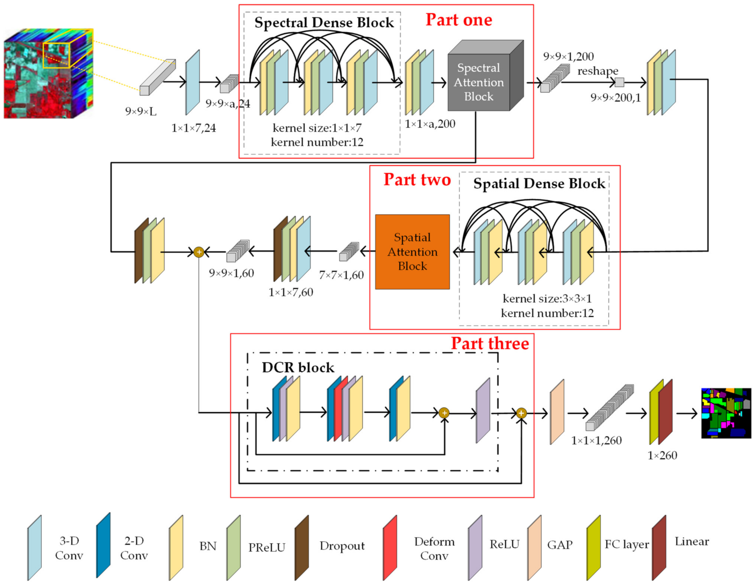
In this section, firstly, the overall framework of the proposed SSAF-DCR network, which consists of three parts, is introduced. The first part is used for spectral feature extraction and selection in order to highlight important spectral features. The second part is used to input the extracted features of the first part into a deep network and then fully extract the spatial features of an HSI. In the third part, a DCR block is designed to adapt to unknown changes and adjust the receptive field, which can further extract spatial features. In addition, a series of optimization methods are adopted to prevent the overfitting phenomenon and to improve the accuracy.
2.1. The Overall Structure of the Proposed Method
The proposed SSAF-DCR network consists of three parts, which are shown in Figure 1. Motivated by the basic structure of the DenseNet [40] and the idea of spectral feature multiplexing, two dense blocks with three convolutional layers are utilized to extract spectral features and spatial features, respectively. First, a dense block with three convolutional layers is used to realize the deep extraction of spectral features. Then, in order to effectively select the important features from the large amount of spectral information, we introduce the channel attention mechanism from the DANet [41] to obtain more effective spectral features. In the second part, similarly to the spectral feature extraction, the feature maps that contain the effective spectral features are sent to another dense block, and the spatial attention mechanism is used to implement the spatial neighborhood feature extraction. In the third part, the feature maps obtained in the first two parts are added element by element. After dimensionality reduction, the results are input into the DCR block to further extract the high-level spatial features. Finally, the extracted high-level features are fed into a global average pooling (GAP), fully connected layer, and linear classifier to obtain the classification results.
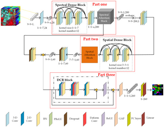
Figure 1.
The overall framework of the proposed SSAF-DCR network.
In this study, the proposal of the DCR block is motivated by DHCNet [26] and by residual networks (ResNets) [42]. The DCR block is generated by combining a deformable convolution layer with a traditional convolution and residual branch. Part D of this section provides a comparison of the results of the classification accuracy and the numbers of parameters with and without the DCR block. This block is utilized to further extract high-level spatial features, which can not only extract spatial features more fully but also prevent the classification accuracy from decreasing with increases in the network depth.
2.2. Dense Spectral and Spatial Blocks
As is commonly known, in recent years, the improvement of convolution neural networks was mainly through the adoptions of ways of widening or deepening the networks. The disappearance of the gradient is the main problem when a network is deepened. Dense blocks not only alleviate the gradient disappearance phenomenon but also reduce the number of parameters. Dense blocks also allow features to be reused by establishing dense connections between all of the previous layers and later layers.
Suppose that an image is propagated in a convolutional network. represents the number of the layer, and represents the output of layer . A traditional feed-forward network takes the output of the layer, , as the input of the layer to obtain the output of the layer, , which can be represented as
For a dense block, each layer obtains additional inputs from all the preceding layers and passes on its own feature maps to subsequent layers; thus, it connects all layers by directly matching the sizes of the feature maps with each other. It can be defined as
Similarly to the dense block, a dense spectral block is utilized in the spectral domain, and the input of the current layer is the cascade of all outputs of the previous layer. Traditional density connectivity uses a two-dimensional CNN to extract features, while the dense spectral block uses a three-dimensional CNN to extract all features of a spectrum, which is more suitable for the structural features of HSIs. The neighborhood pixels of the central pixel are selected from the original HSI data to generate a 3D cube set. If the target pixel is at the edge of the image, the value of the missing adjacent pixel is set to zero. Then, the neighborhood of the image patches around the labeled pixels is obtained and fed into the first part.
We assume that the dense spectral block contains layers, and each layer implements a nonlinear transformation . More specifically, is a composite function of batch normalization (BN) [43], PReLU [44], three-dimensional convolution, and dropout [45]. It should be noted that, because dense connections are realized directly across channels, it is required that the sizes of their feature maps before different layers of concatenation are the same.
For the dense spectral block, the inputs are patches with a size of that are centered on the labeled pixel selected from the original image. In this block, a 1 × 1 × 7 convolution kernel is used for feature extraction in order to obtain the spectral features. The number of convolution kernels is 12. The BN layer and PReLU follow after the convolutional layer. For the dense spatial block, the input samples are patches with a size of that are centered on the labeled pixel selected from the first part after a reshaping operation, where refers to the convolution kernel size, and refers to the stride. In this block, a 3 × 3 × 1 convolution kernel is used to obtain the spatial features. The number of convolution kernels, the normalization method, and the activation function are all the same as those for the dense spectral blocks.
This dense connection makes the transmission of spectral–spatial features and gradients more efficient, and the network is easier to train. Each layer can directly utilize the gradient of the loss function and the initial input feature map, which is a kind of implicit deep supervision, so that the phenomenon of gradient disappearance can be alleviated. The dense convolution block has fewer parameters than a traditional convolutional block because it does not need to relearn redundant feature maps. The traditional feed-forward structure can be regarded as an algorithm for state transfer between layers. Each layer receives the state of the previous layer and passes the new state to the next layer. The dense block changes the state, but it also conveys information that needs to be retained.
2.3. Spectral–Spatial Self-Attention Block and Fusion Mechanisms
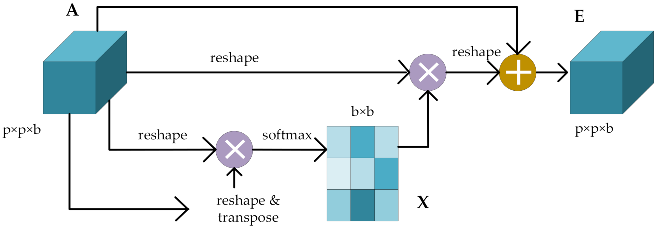
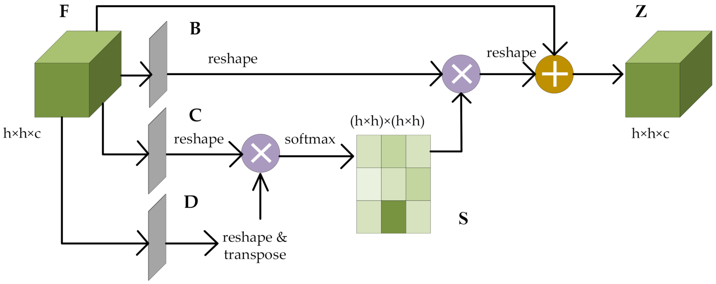
Different spectral bands and spatial pixels have different contributions to HSI classification. In this study, the self-attention mechanism is adopted in order to focus on the features that significantly contribute to the classification results and ignore the unimportant information. According to the feature dependence of the spatial dimension and channel dimension that are captured by the self-attention mechanism, the spectral and spatial features extracted from dense blocks are refined and optimized, with more attention being paid to important features and less attention to unimportant features. Figure 2 and Figure 3 show the schematic diagrams of the attention blocks. This study designed a residual-like method that not only alleviates the phenomenon of gradient disappearance but also enhances the spectral–spatial feature representation, which is essential for the accurate classification of pixels.

Figure 2.
The schematic diagram of the spectral attention block.

Figure 3.
The schematic diagram of the spatial attention block.
For the spectral attention mechanism, the spectral feature map of each high-level feature can be regarded as a class-specific response. By mining the interdependence between the spectral feature maps, the interdependent feature maps can be highlighted, and the feature representations of specific semantics can be improved. The input is a set of feature maps with size , where refers to the patch size, and is the number of input channels. is the spectral attention map with size , which is calculated directly from the original feature map . The specific formula for calculating the spectral attention diagram is
where measures the effect of the th spectral feature on the th spectral feature. The output calculation of the final attention map is
represents the scale coefficient, which is initialized with 0 and gradually learns to assign greater weights. The resulting feature for each spectral channel is the weighted sum of all spectral channels’ features and the original spectral features.
For the spatial attention mechanism, by establishing rich contextual relations of the local spatial features, the broader contextual information can be encoded into the local spatial features in order to improve the feature representation abilities. The size of input is in which refers to , and is the number of input channels. is the spatial attention map with size , calculated from the original spatial feature map . The output formulas of the spatial attention diagram and the final attention map are similar to those of the spectral attention block, as shown in Formulas (5) and (6), respectively. Among them, , , and represent the feature maps obtained by the three convolutions, is the spatial attention map, and and represent the input feature map and the final output feature map, respectively.
2.4. Strategy for High-Level Spatial Feature Extraction—DCR Block
CNNs are often seen as an effective way to automatically learn abstract features through a stack of layers. However, there are a large number of mixed pixels in hyperspectral images. One of the problems of a traditional convolution kernel with a fixed size is its poor adaptability to unknown changes and its weak generalization ability. Therefore, it is difficult to fully learn the features of an HSI through only regular convolution. In order to solve the above problems and ensure that the classification accuracy does not decrease as the network deepens, a DCR block is proposed. The parameter settings of each layer of DCR block are shown in Table 1. The process of implementing deformable convolution is shown in Figure 4. First, a feature map is obtained through a traditional convolutional layer; then, the result is input to another convolutional layer to obtain offset features, which correspond to the original output feature and the offset feature, respectively. The output offset size is consistent with the input feature map size. The dimension of the generated channel is , which is twice the number of convolution kernels. The original output feature and the offset feature are simultaneously learned through the bilinear interpolation backpropagation algorithm. The shape of the traditional convolution operation is regular and can be represented as
where is the pixel of the output feature map, and represents the locations in the enumerated convolution kernel. The deformable convolution is

Table 1.
Parameter settings of the DCR block of the residual part.
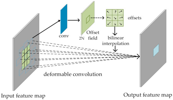
Figure 4.
The implementation process for deformable convolution.
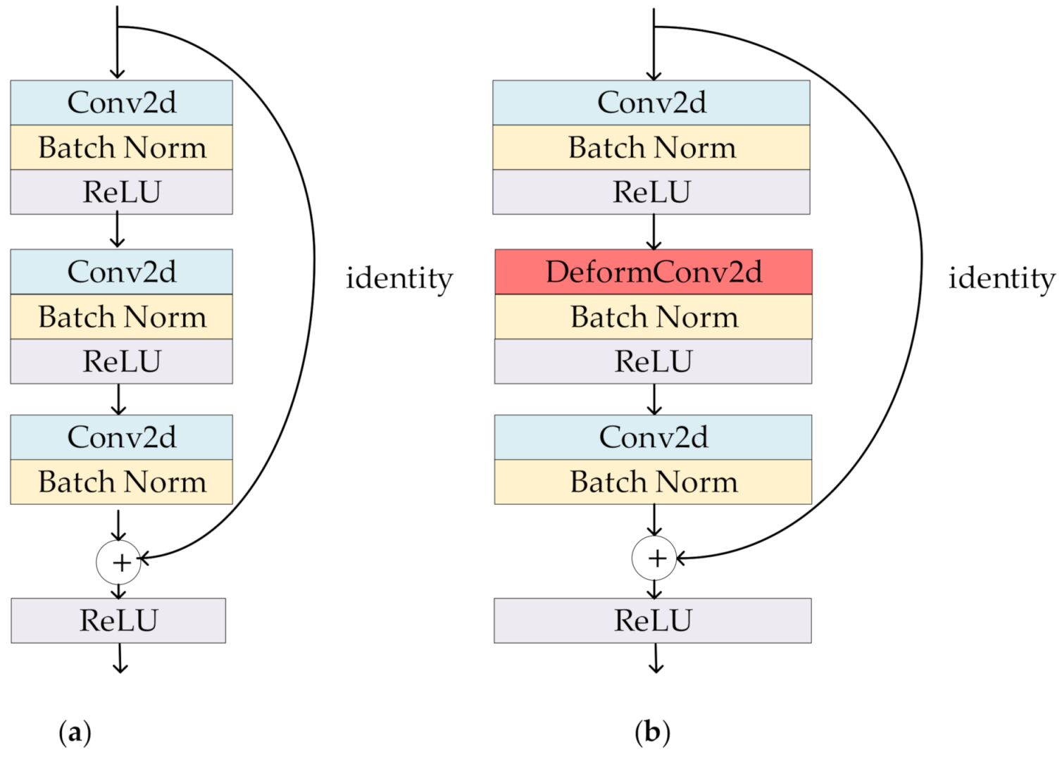
The offset is added to the original position in Formulas (7) and (8). , , and represent the weight, input feature map, and output feature map, respectively. The schematic diagram of the original three-layer residual block and the proposed DCR block are shown in Figure 5a,b. By introducing residual learning into the deep network’s structure, the generalization performance of the network is improved. In this study, residual learning was used in two places—one is in the DCR block, and the other is the residual between the feature map after the self-attention fusion and the DCR block. This can solve the degradation problem caused by increasing the depth of network and can make the network easier to optimize. This residual block is divided into two parts: (1) the direct mapping part and (2) the residual part. The residual part can be represented as
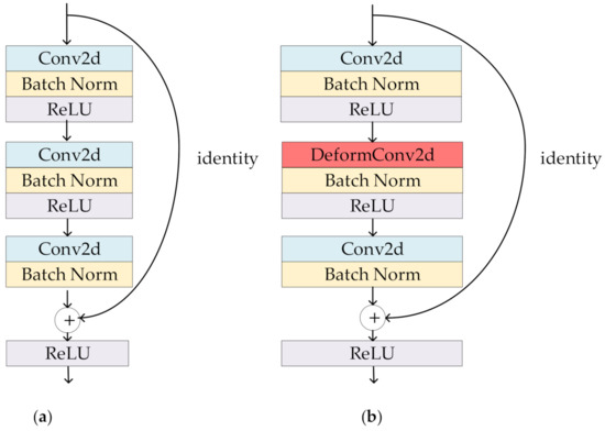
Figure 5.
Architectures of (a) the ordinary residual block and (b) the proposed DCR block.
Because the number of feature maps of and is the same, is the identity map, that is, , which is reflected as the arc on the right side of Figure 5b; is the residual part, which consists of two regular convolutions and one deformable convolution, followed by BN layers and a ReLU layer [46], which corresponds to the part with convolution on the left side of Figure 5b, where and are the input feature map and weight.
2.5. Optimization Methods
In order to accelerate the training speed, improve the classification accuracy, and prevent overfitting, some optimization approaches are adopted, including the PReLU activation function [44], BN, dropout, and cosine-annealing learning rate monitoring mechanism.
- (1)
- PReLU Activation Function
PReLU is an improvement and generalization of ReLU; its name refers to ReLU with parameters. The PReLU can be represented as
where is the input of the nonlinear activation function of the th channel, and is the slope of the activation function in the negative direction. For each channel, there is a learnable parameter for controlling the slope. When updating the parameter , the momentum method is adopted. That is,
here, is the momentum coefficient, and is the learning rate. The weight decay is not used in the update because it will cause to tend to zero. In addition, all values of at the initial moment are equal to 0.25. The Mish [47] is
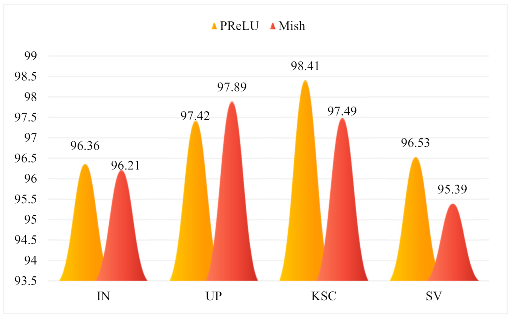
here, represents the input of the activation. Moreover, Mish has a smoother gradient compared to that of ReLU. Figure 6 shows the comparison results of the overall classification accuracy on each dataset using Mish or PReLU. It can be seen from Figure 6 that the overall accuracies on the three datasets with the PReLU activation function are all higher than those with the Mish activation function. Therefore, PReLU was adopted in this study.
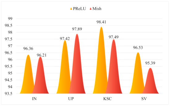
Figure 6.
The overall accuracy (%) with different activation functions.
- (2)
- Cosine-Annealing Learning Rate
The learning rate is one of the most important hyperparameters of deep neural networks, and it controls the speed of the weight update. A high at the beginning of training is used to quickly approach the optimal value, but if it is not reduced later, it is likely to update to a point that exceeds the optimal value or oscillate near the optimal point. Therefore, adjusting the value of is a way to make the algorithm faster on the premise of ensuring accuracy. The cosine-annealing learning rate is utilized to dynamically adjust the learning rate. It can be represented as
where is the newly obtained learning rate, is the initial learning rate, represents the minimum learning rate, represents the current number of iterations, and represents the maximum number of iterations. In this study, is set to 10.
- (3)
- Other Optimization Approaches
BN has been widely used in deep neural network training; it can not only accelerate the convergence speed of the model, but more importantly, it can also alleviate the problem of scattered feature distribution in the deep network.
During forward propagation, dropout causes the activation value of a certain neuron to stop working with a certain probability because it does not rely too much on certain local features, which can make the model more general. A dropout layer [43] is used after the spatial attention block and the spectral attention block, and = 0.5.
The early stop strategy estimates the stop loss standard by using the validation loss. The upper limit is set to 200 epochs. If the loss in the validation set no longer declines for 20 epochs, then the training phase is terminated. Finally, the parameters from the results of the last iteration are used as the final parameters of the model. The proposed SSAF-DCR method is described as follows (Algorithm 1).
| Algorithm 1 The SSAF-DCR model |
| Input: An HSI dataset and the corresponding label vectors . |
| Step 1: Extract cubes with a patch size of 9 × 9 × L from , where is the number of spectral bands. |
| Step 2: Randomly divide the HSI dataset into , , and , which represent the training data, validation data, and testing data, respectively. Likewise, , , and are the corresponding label vector data for , , and . |
| Step 3: Input , and , into the initial SSAF-DCR model. |
| Step 4: Calculate the dense blocks according to (2) to initially obtain the effective features. |
| Step 5: Selectively filter features according to (3)–(5), and (6). |
| Step 6: Further extract spatial features according to (8) and (9). |
| Step 7: Adam is used for iterative optimization. |
| Step 8: Input into the optimal model to predict the classification results. |
| Output: The classification results. |
3. Experimental Results and Analysis
3.1. Dataset
In this study, four classical HSI datasets, i.e., the Indian Pines (IN), the Pavia University (UP), the Kennedy Space Center (KSC), and the Salinas Valley (SV) datasets, were used to verify the performance of the proposed method.
The Indian Pines dataset was acquired by the AVIRIS sensor in Indiana. The size of this dataset is 145 × 145 with 224 bands, including 200 effective bands. There are 16 crop categories. The Pavia University dataset was obtained by the ROSIS sensors and is often used for hyperspectral image classification. The sensor has a total of 115 bands. After processing, the University of Pavia dataset has a size of 610 × 340 with 103 bands and a total of nine ground features. The KSC dataset was captured by the AVIRIS sensor at the Kennedy Space Center in Florida on 23 March 1996. The size of this dataset is 512 × 614; 176 bands remain after the water-vapor noise is removed, the spatial resolution is 18 m, and there are 13 categories in total. The Salinas dataset was taken by an AVIRIS sensor in the Salinas Valley in California. The spatial resolution of the dataset is 3.7 m, and the size is 512 × 217. The original dataset has 224 bands, and 204 bands remain after removing noise. This dataset contains 16 crop categories.
In this study, 3% of the samples of the IN dataset are randomly selected as the training set, and the remaining 97% are used as the test set. In addition, 0.5% of the samples of the UP dataset are randomly selected as the training set, and the remaining 99.5% are used as the test set. The selection proportions of the training set and test set of the SV dataset are the same as those of the UP dataset. For the KSC dataset, 5% of the samples are selected for training and 95% for the test set. The batch size of each dataset is 32. As is commonly known, the more training samples there are, the higher the accuracy is. In the next section, we verify that our proposed method also shows great performance in the case of minimal training samples. The number of training samples and test samples of different datasets are listed in Table 2, Table 3, Table 4 and Table 5, respectively.
Table 2.
Number of training and test samples in the IN data set.
Table 3.
Number of training and test samples in the UP data set.
Table 4.
Number of training and test samples in the KSC data set.
Table 5.
Number of training and test samples in the SV data set.
3.2. Parameter Setting and Experimental Results
The experimental hardware platform was a server with an Intel (R) Core (TM) i9–9900K CPU, NVIDIA GeForce RTX 2080 Ti GPU, and 32 GB random-access memory. The experimental software platform was based on the Windows 10 Visual Studio Code operating system with CUDA10.0, Pytorch 1.2.0, and Python 3.7.4. All experiments are repeated ten times with different randomly selected training data, and the average results are given. The optimizer was set to Adam with a learning rate of 0.0003. The overall accuracy (OA), average accuracy (AA), and kappa coefficient (Kappa) were chosen as the classification evaluation indicators in this study. Here, OA represents the ratio of the number of correctly classified samples to the total number of samples, AA represents the classification accuracy of each category, and the kappa coefficient measures the consistency between the results and the ground truth. The performance of the proposed method was compared with those of some state-of-the-art CNN-based methods for HSI classification, including KNN [48], SVM-RBF [49], CDCNN [50], SSRN [38], FDSSC [51], DHCNet [26], DBMA [52], HybridSN [39], DBDA [32], and LiteDepthwiseNet [53], where KNN is a linear model and SVM_RBF uses radial basis function to solve the nonlinear classification problem. The above two methods belong to traditional classification methods. Both CDCNN and DHCNet are 2DCNN models, and other methods, including the proposed method, are 3DCNN models.
The training samples of the four datasets selected for all methods were the same. Table 6, Table 7, Table 8 and Table 9 list the class-specific accuracy of all the methods for the IN, UP, KSC, and SV datasets. In addition, among the eleven algorithms, the best results are highlighted in bold. All of the results are the average results over ten experiments. As can be observed, the proposed method provided the best OA, AA, and Kappa, with a significant improvement over the other methods on the four datasets. In Table 6, the results show that the proposed method has the highest OA value, reaching 96.36%, with gains of 40.75%, 18.78%, 34.16%, 3.04%, 1.57%, 1.17%, 6.58%, 8.9%, 1.04%, and 0.77% over the KNN, SVM-RBF, CDCNN, SSRN, FDSSC, DHCNet, DBMA, HybridSN, DBDA, and LiteDepthwiseNet methods, respectively. KNN hardly uses shallow spectral features and ignores rich spatial features, resulting in poor classification effect. The SVM-RBF method does not utilize spatial neighborhood information; thus, its OA was 77.58%. However, CDCNN was worse than SVM-RBF with an OA of more than 15% because the network structure has poor robustness. The FDSSC method adopts dense connection, which caused it to have an OA that was over 1.47% greater than that of the SSRN with residual connection. DBMA extracted features with two branches and a multi-attention mechanism, but the classification results were still lower than those of FDSSC because the use of too few training samples resulted in serious overfitting. DHCNet introduces deformable convolution and deformable downsampling, and it fully considers the dependence of spatial context information; its OA was 0.4% higher than that of FDSSC, and its AA was up to 2% higher than that of FDSSC. HybridSN network has few parameters, but its structure is too simple, which leads to insufficient extraction of spectral–spatial information, so its OA value is 8.9% lower than that of the proposed method. The DBDA network—with dual branches and dual attention—has a relatively flexible feature extraction structure, so its OA was higher than those of the aforementioned networks. LiteDepthwiseNet has a slightly longer number of layers and lacks fine extraction of spectral spatial features. Therefore, the classification accuracy is slightly lower than that of the proposed method. Because the proposed method has dense blocks to achieve effective spectral–spatial feature extraction, attention blocks to selectively filter and aggregate features, DCR block to achieve deep spatial feature extraction, and a series of optimization methods, the SSAF-DCR framework we proposed achieves the best performance. For the UP and KSC datasets, the OAs of DBMA were all lower than those of DHCNet, DBDA, and the proposed method, and the classification results of other methods in the other three data sets are also similar to the results in Table 6, as shown in Table 7 and Table 8. For the SV data sets with clear category boundaries, as shown in Table 9, the OA value of LiteDepthwiseNet is only 0.31% less than that of the proposed SSAF-DCR method, which is all higher than that of the other nine methods. In addition, the classification results of the object-based HSI method are also compared with those of the proposed method. For the UP data set, when 50 samples of each class are randomly selected as training sets, the OA obtained in [11] is 95.33%, AA is 94.23%, and kappa is 0.92; The OA, an, and kappa of the proposed SSAF_DCR method are 98.39%, 97.26%, and 0.97, respectively; it is 3.06%, 3.03%, and 0.05 higher than the value in [11]. For SV data set, 10% are randomly selected as training sets. The OA value obtained by the proposed SSAF_DCR method is 99.71%, which is 0.45% higher than the OA value in [11]. The classification maps of different methods on the Pavia University dataset and the Indian Pines dataset are provided to further validate the performance of the proposed SSAF-DCR network, as shown in Figure 7, Figure 8, Figure 9 and Figure 10. It can be seen that the classification maps of the SSAF-DCR network have less noise, and the boundaries of the objects are clearly defined. Compared with the other methods, the classification maps of the SSAF-DCR network on the four datasets are closest to the ground-truth maps. The above experiments prove the effectiveness of the proposed SSAF-DCR network. However, this method still has some shortcomings. Since the feature extraction structure of SSAF-DCR contains three different parts, more discriminative information can be obtained, and the highest accuracy can be obtained under the minimum training samples. However, the depth of the model is relatively deep, so the test time is relatively long.
Table 6.
KPI (OA, AA, Kappa) on the Indian Pines (IN) dataset with 3% training samples.
Table 7.
KPI (OA, AA, Kappa) on the University of Pavia (UP) dataset with 0.5% training samples.
Table 8.
KPI (OA, AA, Kappa) on the Kennedy Space Center (KSC) dataset with 5% training samples.
Table 9.
KPI (OA, AA, Kappa) on the Salinas Valley (SV) dataset with 0.5% training samples.
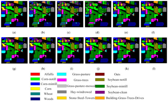
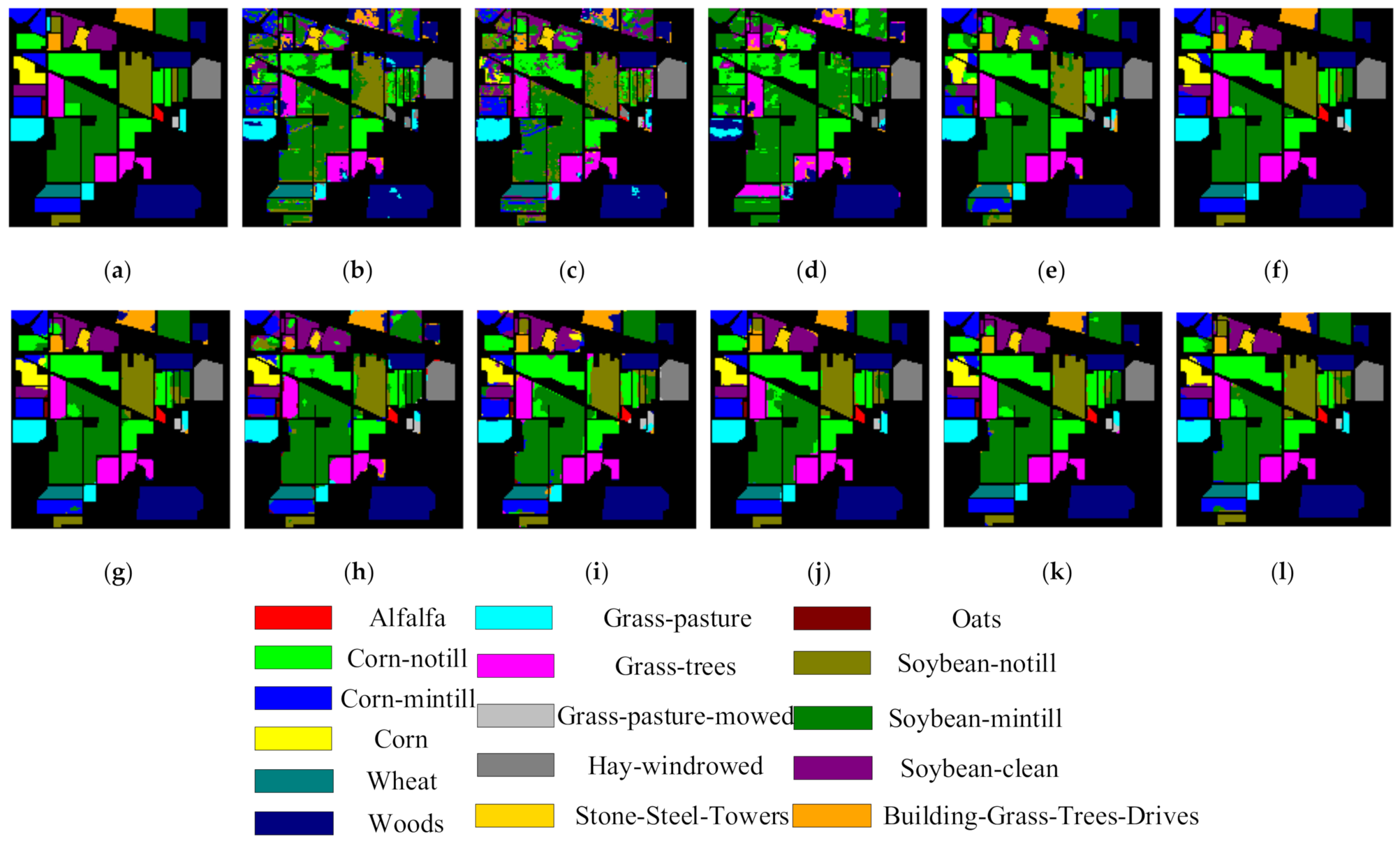
Figure 7.
Full classification maps on the Indian Pines image obtained with the (a) ground truth, (b) KNN (OA = 55.61), (c) SVM-RBF (OA = 77.58), (d) CDCNN (OA = 62.20), (e) SSRN (OA = 93.32), (f) FDSSC (OA = 94.79), (g) DHCNet (OA = 95.19), (h) DBMA (OA = 89.78), (i) HybridSN (OA = 87.46), (j) DBDA (OA = 95.45), (k) LiteDepthwiseNet (OA = 95.59), and (l) proposed method (OA = 96.36).
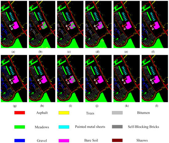
Figure 8.
Full classification maps on the University of Pavia images obtained with the (a) ground truth, (b) KNN (OA = 68.21), (c) SVM-RBF (OA = 81.84), (d) CDCNN (OA = 86.89), (e) SSRN (OA = 95.66), (f) FDSSC (OA = 94.72), (g) DHCNet (OA = 96.29), (h) DBMA (OA = 95.72), (i) HybridSN (OA = 92.83), (j) DBDA (OA = 96.47), (k) LiteDepthwiseNet (OA = 96.60), and (l) proposed method (OA = 97.43).
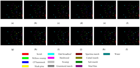
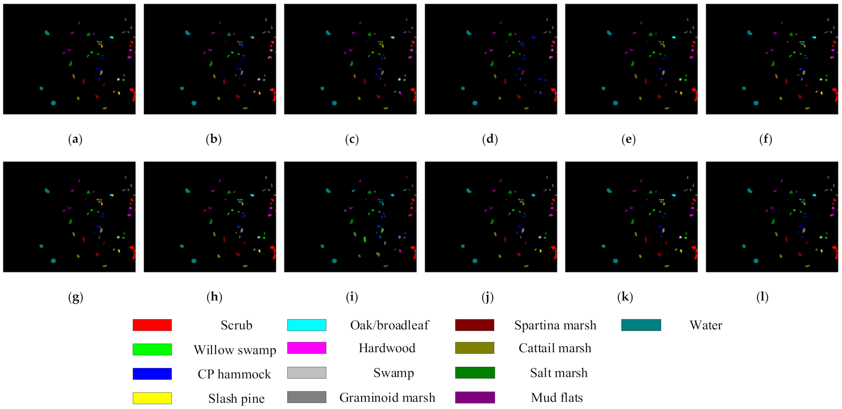
Figure 9.
Full classification maps on the Kennedy Space Center images obtained with the (a) ground truth, (b) KNN (OA = 79.98), (c) SVM-RBF (OA = 84.97), (d) CDCNN (OA = 80.91), (e) SSRN (OA = 96.06), (f) FDSSC (OA = 97.58), (g) DHCNet (OA = 97.41), (h) DBMA (OA = 95.07), (i) HybridSN (OA = 63.72), (j) DBDA (OA = 97.59), (k) LiteDepthwiseNet (OA = 97.41), and (l) proposed method (OA = 98.41).
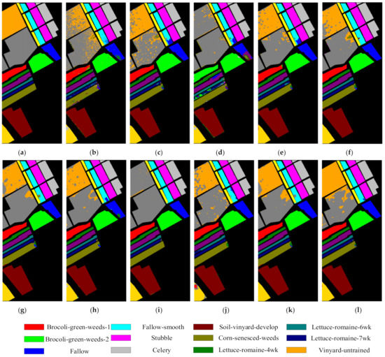
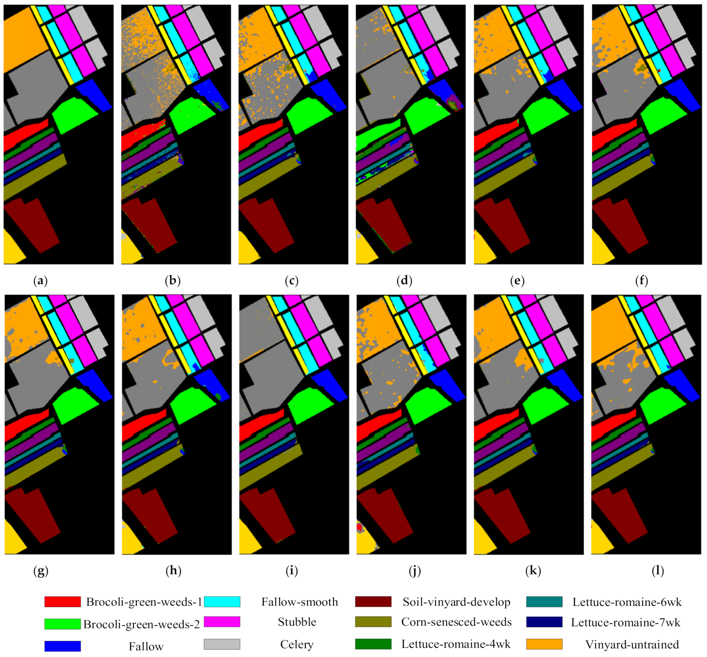
Figure 10.
Full classification maps on the Salinas Valley images obtained with the (a) ground truth, (b) KNN (OA = 82.17), (c) SVM-RBF (OA = 88.09), (d) CDCNN (OA = 80.51), (e) SSRN (OA = 90.11), (f) FDSSC (OA = 94.60), (g) DHCNet (OA = 94.45), (h) DBMA (OA = 92.62), (i) HybridSN (OA = 95.05), (j) DBDA (OA = 95.81), (k) LiteDepthwiseNet (OA = 97.02), and (l) proposed method (OA = 97.46).
3.3. Efficiency of the Attention Fusion Strategy
The purpose of feature fusion is to merge the features extracted from the image into a feature that is more discriminative than the input feature. According to the order of fusion and prediction, feature fusion is classified into early fusion and late fusion. Early fusion is a commonly used classical feature fusion method, that is, in existing networks (such as the Inside–Outside Net (ION) [54] or HyperNet [55]), concatenation [56] or addition operations are used to fuse certain layers. The residual-like feature fusion strategy designed in this study is an early fusion strategy that directly connects two spectral and spatial scale features. The sizes of the two input features are the same, and the output feature dimension is the sum of the two dimensions. Table 10 shows an analysis of the effects of using the fusion strategy or not. The bold values in Table 10 are the OA values obtained on the four data sets by the proposed method after using the fusion strategy. It can be seen that the OA values on each data set have increased by more than 2% with fusion. The results show that the effect on the classification of hyperspectral images is significantly improved after feature fusion compared with that without the feature fusion strategy.
Table 10.
Effective analysis of the attention blocks fusion strategy (OA%).
3.4. Parameter Analysis
In this section, the impacts of different spatial patch sizes on the classification accuracy and the impacts of different training samples on the performance of the proposed method are analyzed.
(1) It is well known that a target spectral pixel and its surrounding spatial neighborhood usually belong to the same category. Therefore, the spatial size of the input cube has a great impact on the classification performance. If the spatial size of the input cube is too small, the receiving field for feature extraction will be insufficient, resulting in a loss of information and reduced classification performance; if it is too large, the local spatial features cannot be effectively extracted, and the computational cost and memory demand will be drastically increased. Figure 11 shows the OA values of the four datasets with different patch sizes, which varied from 5 × 5 to 9 × 9 with an interval of 2. In Figure 11, as the spatial size of the input cube increases, the OAs of the IN, UP, and KSC datasets begin to decline after 7 × 7, where they reach the highest values of 96.36%, 97.42%, and 98.41%, respectively. For the SV dataset, the OA keeps increasing as the spatial size of the input cube increases. Through the analysis of the experimental results on the four datasets, it was found that the 7 × 7 spatial patch size was able to provide the best performance, so this study used 7 × 7 as the spatial input size.
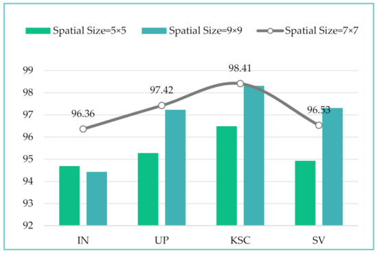
Figure 11.
Overall accuracy (%) of input patches with different spatial sizes on the four datasets.
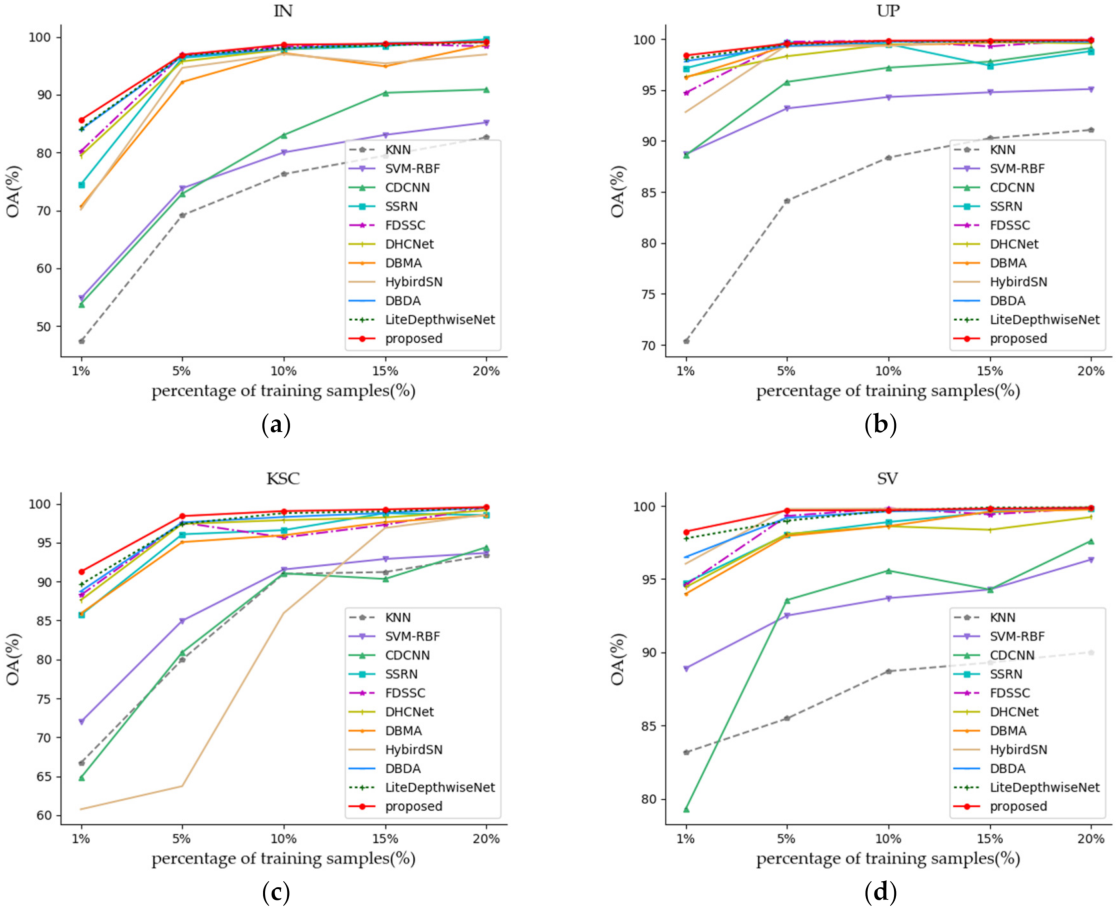
(2) Figure 12a–d shows all of the methods that were investigated with different numbers of training samples. Specifically, training samples of 1%, 5%, 10%, 15%, and 20% of each class of the IN and KSC datasets were randomly selected from the labeled samples, and 0.5%, 5%, 10%, 15%, and 20% of the training samples in each category of the UP and SV datasets were randomly selected from the labeled samples. It can be seen from Figure 12 that the proposed SSAF-DCR method obtains the highest OA values on all four data sets under the condition of minimum training samples. With the increase of training proportion, the OA values of all methods are improved to varying degrees, and the performance differences between different models are also reduced, but the OA value of the proposed method is still the highest. In general, the 3D-CNN-based models (including SSRN [38], FDSSC [51], DBMA [52], DBDA [32], and the proposed model) showed better performance compared to the other methods. Among them, the proposed SSAF-DCR method always had the optimal OA value under the different training sample ratios. Therefore, our proposed method has a stronger generalization ability when training on a hyperspectral dataset with limited samples.
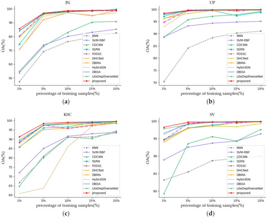
Figure 12.
Classification results (OA%) with different amounts of training samples on four datasets. (a) IN. (b) UP. (c) KSC. (d) SV.
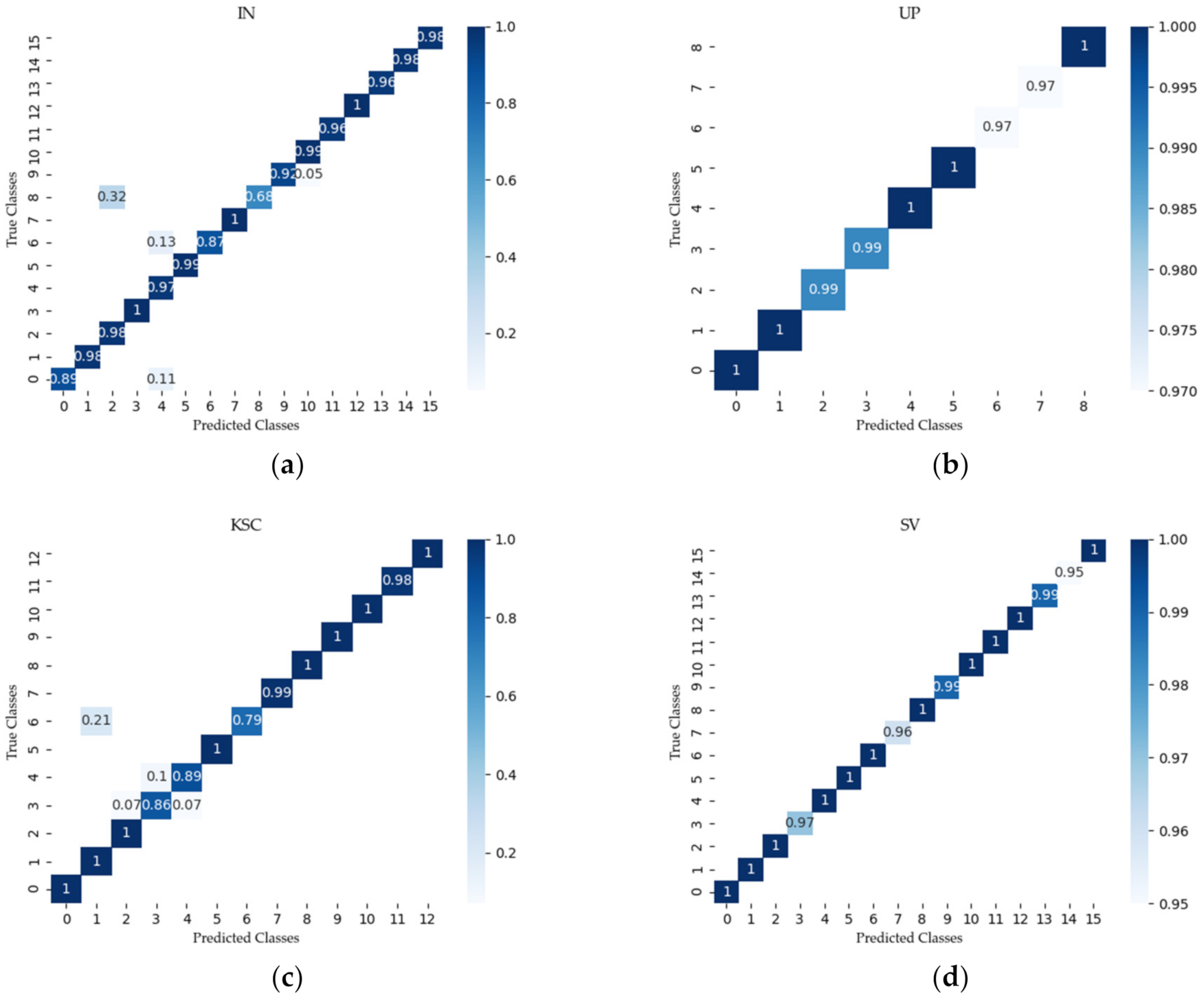
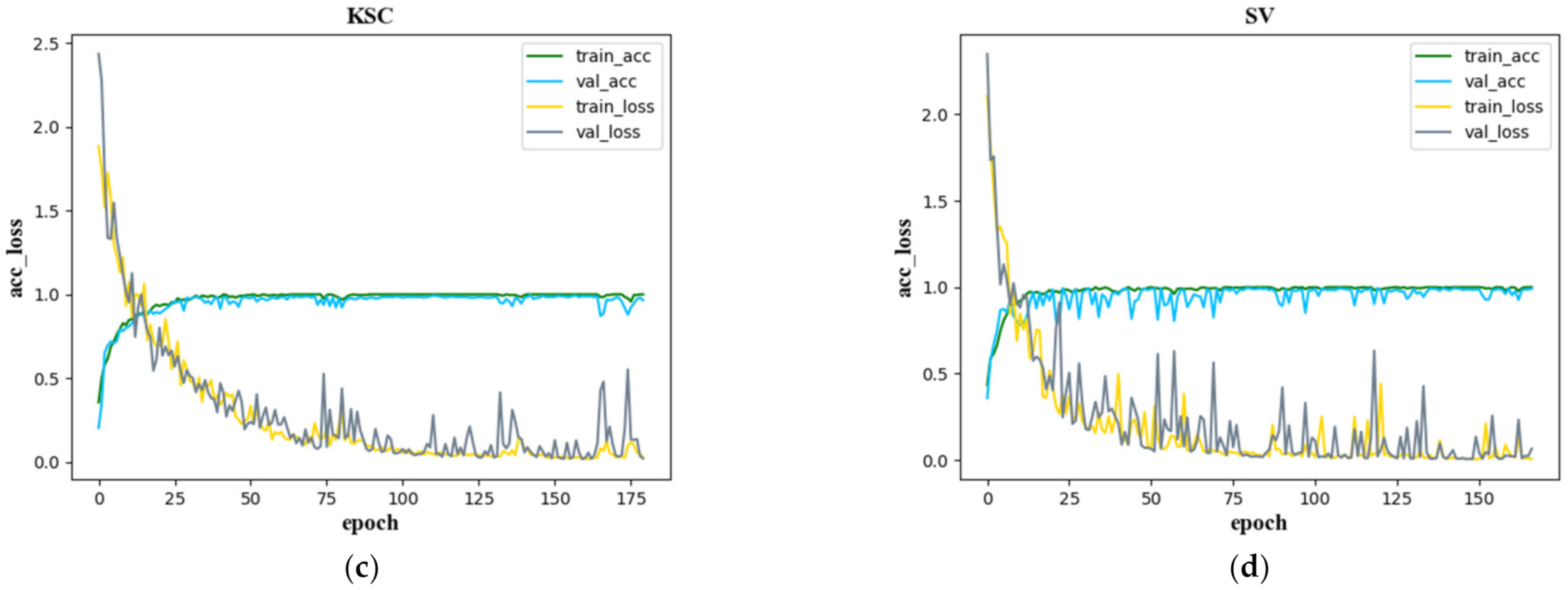
Figure 13 shows the confusion matrix created with the proposed SSAF-DCR method on the IN, UP, KSC, and SV datasets, respectively. The accuracy and loss curves of the SSAF-DCR training and verification sets for the IN, UP, KSC, and SV datasets are shown in Figure 14. For the UP and SV datasets, there were large fluctuations in the losses of the validation set, but the SSAF-DCR model converged quickly at the beginning of the training process, so good results were still achieved for the training and validation accuracy.

Figure 13.
Confusion matrix using the proposed method for (a) IN, (b) UP, (c) KSC, and (d) SV.
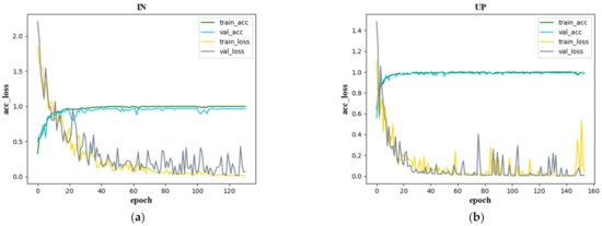
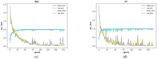
Figure 14.
Accuracy and loss function curves of the training and validation sets for (a) IN, (b) UP, (c) KSC, and (d) SV.
3.5. Ablation Experiments of Three Kinds of Blocks
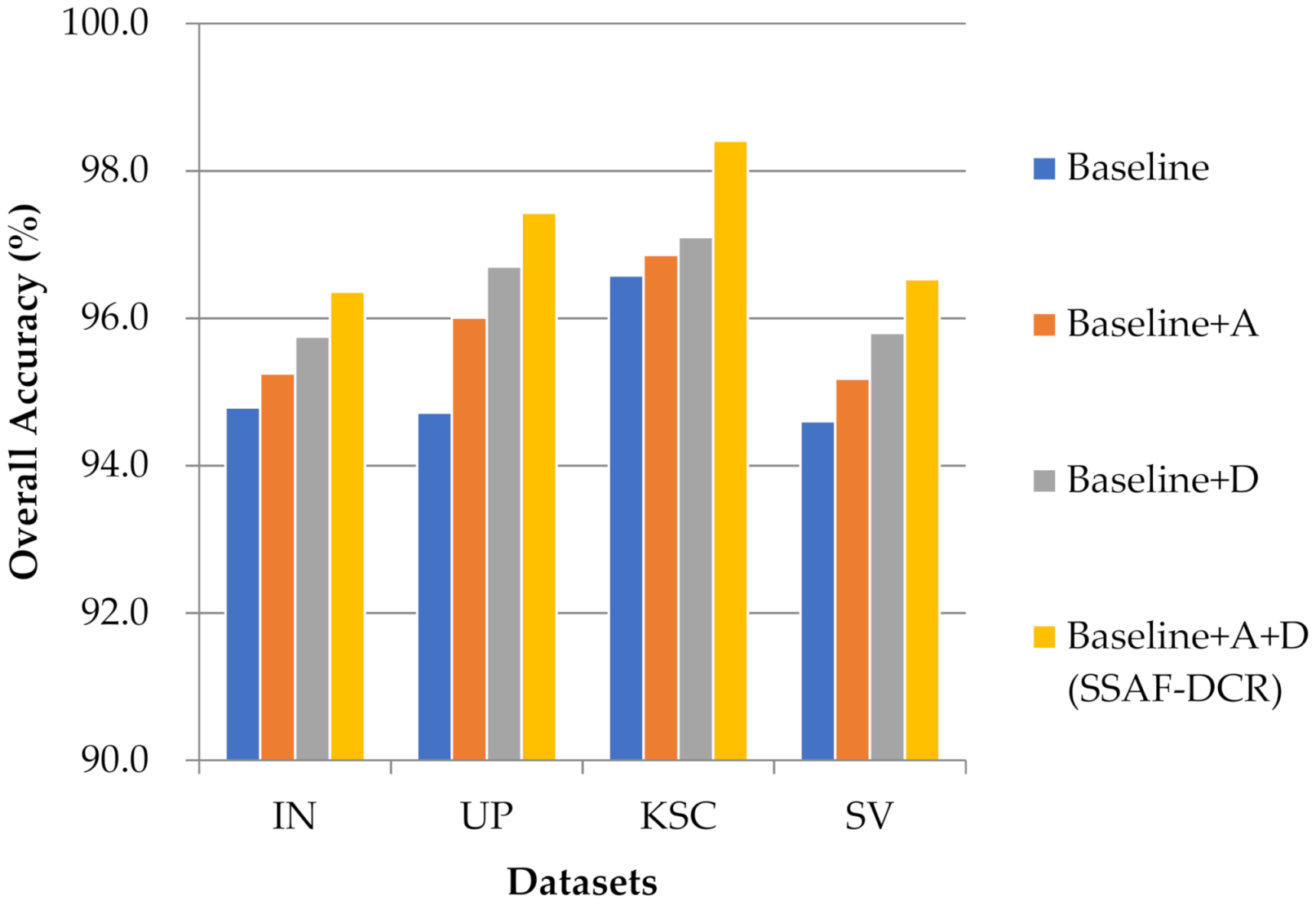
The proposed method uses three modules: dense blocks, attention blocks, and DCR block. In order to verify their respective performance, in this paper, the network composed of two dense blocks is taken as the baseline network. On this basis, attention blocks (abbreviated as A) and DCR block (abbreviated as D) are respectively added to form the baseline + A network and baseline + D network. Attention blocks and DCR block are also together added to the baseline network to form a baseline + A+ D network (i.e., the proposed SSAF-DCR network). The ablation experiments and analyses of these three networks were performed on four data sets as shown in Figure 15. It can be seen that because the DCR block has made effective adjustments to the receptive field, it has better adapted to spatial changes and further extracted spatial features; while the attention block has selectively screened and aggregation the previously extracted features, so only adding the DCR block has an improvement in the OA value on the four data sets compared to only adding the attention block. Due to the good combination of the advantages of attention block and DCR block in feature extraction, it is obvious that the baseline + A + D network (i.e., the proposed SSAF-DCR network) composed of the two achieves the best classification accuracy on the four datasets.
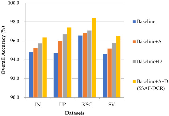
Figure 15.
Schematic of the ablation results about attention blocks and DCR block on the four data sets.
4. Conclusions
In this study, a novel lightweight SSAF-DCR method was proposed for hyperspectral image classification. The SSAF-DCR method first uses a dense spectral block for effective spectral domain feature extraction. Secondly, a spectral attention block is used to focus on more interesting features and ignore unimportant information. Again, the dense spatial block can extract as much information as possible in the spatial domain. It also uses the spatial attention block to selectively filter and discriminate among features. Moreover, a residual-like fusion strategy was designed to fuse the effective features extracted from the spectral domain and the spatial domain, which further enhances the feature representation. In SSAF-DCR, a DCR module was also designed in order to combine the traditional and deformable convolution and embed them into the residual structure to adapt to unknown spatial changes and enhance the generalization ability. These designs are integrated into a unified end-to-end framework to improve the HSI classification performance. The experimental results prove the effectiveness of the SSAF-DCR method.
Author Contributions
Conceptualization, C.S.; data curation, C.S. and T.Z.; formal analysis, D.L.; methodology, C.S.; software, T.Z.; validation, C.S. and T.Z.; writing—original draft, T.Z.; writing—review and editing, C.S. and L.W. All authors have read and agreed to the published version of the manuscript.
Funding
This research was funded in part by the National Natural Science Foundation of China (41701479, 62071084), in part by the Heilongjiang Science Foundation Project of China under Grant JQ2019F003, and in part by the Fundamental Research Funds in Heilongjiang Provincial Universities of China under Grant 135509136.
Data Availability Statement
The Indiana Pines, University of Pavia, Kennedy Space Center and Salinas Valley datasets are available online at http://www.ehu.eus/ccwintco/index.php?title=Hyperspectral_Remote_Sensing_Scenes (accessed on 3 July 2021).
Acknowledgments
We are grateful to the handling editor and the anonymous reviewers for their careful reading and helpful remarks.
Conflicts of Interest
The authors declare no conflict of interest.
References
- Chang, C.I. Hyperspectral Data Exploitation: Theory and Applications; John Wiley & Sons: Hoboken, NJ, USA, 2007. [Google Scholar]
- Patel, N.K.; Patnaik, C.; Dutta, S.; Shekh, A.M.; Dave, A.J. Study of crop growth parameters using airborne imaging spectrometer data. Int. J. Remote Sens. 2001, 22, 2401–2411. [Google Scholar] [CrossRef]
- Goetz, A.F.; Vane, G.; Solomon, J.E.; Rock, B.N. Imaging Spectrometry for Earth Remote Sensing. Science 1985, 228, 1147–1153. [Google Scholar] [CrossRef]
- Civco, D.L. Artificial neural networks for land-cover classification and mapping. Int. J. Geogr. Inf. Syst. 1993, 7, 173–186. [Google Scholar] [CrossRef]
- Ghamisi, P.; Benediktsson, J.A.; Ulfarsson, M.O. Spectral–Spatial Classification of Hyperspectral Images Based on Hidden Markov Random Fields. IEEE Trans. Geosci. Remote Sens. 2013, 52, 2565–2574. [Google Scholar] [CrossRef] [Green Version]
- Farrugia, R.A.; Debono, C.J. A Robust Error Detection Mechanism for H.264/AVC Coded Video Sequences Based on Support Vector Machines. IEEE Trans. Circuits Syst. Video Technol. 2008, 18, 1766–1770. [Google Scholar] [CrossRef] [Green Version]
- Zhong, P.; Wang, R. Jointly Learning the Hybrid CRF and MLR Model for Simultaneous Denoising and Classification of Hyperspectral Imagery. IEEE Trans. Neural Netw. Learn. Syst. 2014, 25, 1319–1334. [Google Scholar] [CrossRef]
- Fang, L.; Li, S.; Kang, X.; Benediktsson, J.A. Spectral-spatial classification of hyper- spectral images with a superpixel-based discriminative sparse model. IEEE Trans. Geosci. Remote Sens. 2015, 53, 4186–4201. [Google Scholar] [CrossRef]
- Fu, W.; Li, S.; Fang, L. Spectral-spatial hyperspectral image classification via superpixel merging and sparse representation. In Proceedings of the 2015 IEEE International Geoscience and Remote Sensing Symposium (IGARSS), Milan, Italy, 26–31 July 2015; pp. 4971–4974. [Google Scholar]
- Fang, L.; Li, S.; Duan, W.; Ren, J.; Benediktsson, J.A. Classification of Hyperspectral Images by Exploiting Spectral–Spatial Information of Superpixel via Multiple Kernels. IEEE Trans. Geosci. Remote Sens. 2015, 53, 6663–6674. [Google Scholar] [CrossRef] [Green Version]
- Zehtabian, A.; Ghassemian, H. An adaptive framework for spectral-spatial classification based on a combination of pixel-based and object-based scenarios. Earth Sci. Inform. 2017, 10, 357–368. [Google Scholar] [CrossRef]
- Addink, E.A.; De Jong, S.M.; Pebesma, E.J. The Importance of Scale in Object-based Mapping of Vegetation Parameters with Hyperspectral Imagery. Photogramm. Eng. Remote Sens. 2007, 73, 905–912. [Google Scholar] [CrossRef] [Green Version]
- Zeng, D.; Liu, K.; Chen, Y.; Zhao, J. Distant Supervision for Relation Extraction via Piecewise Convolutional Neural Networks. In Proceedings of the 2015 Conference on Empirical Methods in Natural Language Processing, Lisbon, Portugal, 17–21 September 2015; pp. 1753–1762. [Google Scholar]
- Gehring, J.; Auli, M.; Grangier, D.; Yarats, D.; Dauphin, Y.N. Convolutional Sequence to Sequence Learning. arXiv 2017, arXiv:1705.03122. [Google Scholar]
- He, H.; Gimpel, K.; Lin, J. Multi-Perspective Sentence Similarity Modeling with Convolutional Neural Networks. In Proceedings of the 2015 Conference on Empirical Methods in Natural Language Processing, Milan, Italy, 26–31 July 2015; pp. 1576–1586. [Google Scholar]
- Li, G.; Li, L.; Zhu, H.; Liu, X.; Jiao, L. Adaptive Multiscale Deep Fusion Residual Network for Remote Sensing Image Classification. IEEE Trans. Geosci. Remote Sens. 2019, 57, 8506–8521. [Google Scholar] [CrossRef]
- Ronneberger, O.; Fischer, P.; Brox, T. U-Net: Convolutional Networks for Biomedical Image Segmentation. In International Conference on Medical Image Computing and Computer-Assisted Intervention; Springer: Cham, Switzerland, 2015; pp. 234–241. [Google Scholar] [CrossRef] [Green Version]
- Wang, R.J.; Li, X.; Ling, C.X. Pelee: A Real-Time Object Detection System on Mobile Devices. arXiv 2018, arXiv:1804.06882. [Google Scholar]
- Sainath, T.N.; Mohamed, A.-R.; Kingsbury, B.; Ramabhadran, B. Deep convolutional neural networks for LVCSR. In Proceedings of the 2013 IEEE International Conference on Acoustics, Speech and Signal Processing, Vancouver, BC, Canada, 26–31 May 2013; pp. 8614–8618. [Google Scholar]
- Hu, W.; Huang, Y.; Wei, L.; Zhang, F.; Li, H.-C. Deep Convolutional Neural Networks for Hyperspectral Image Classification. J. Sens. 2015, 2015, 258619. [Google Scholar] [CrossRef] [Green Version]
- Li, W.; Wu, G.; Zhang, F.; Du, Q. Hyperspectral Image Classification Using Deep Pixel-Pair Features. IEEE Trans. Geosci. Remote Sens. 2016, 55, 844–853. [Google Scholar] [CrossRef]
- Fang, L.; Liu, Z.; Song, W. Deep Hashing Neural Networks for Hyperspectral Image Feature Extraction. IEEE Geosci. Remote Sens. Lett. 2019, 16, 1412–1416. [Google Scholar] [CrossRef]
- He, N.; Paoletti, M.E.; Haut, J.N.M.; Fang, L.; Li, S.; Plaza, A.; Plaza, J. Feature Extraction With Multiscale Covariance Maps for Hyperspectral Image Classification. IEEE Trans. Geosci. Remote Sens. 2019, 57, 755–769. [Google Scholar] [CrossRef]
- Chen, Y.; Li, C.; Ghamisi, P.; Jia, X.; Gu, Y. Deep Fusion of Remote Sensing Data for Accurate Classification. IEEE Geosci. Remote Sens. Lett. 2017, 14, 1253–1257. [Google Scholar] [CrossRef]
- Zhang, M.; Li, W.; Du, Q. Diverse Region-Based CNN for Hyperspectral Image Classification. IEEE Trans. Image Process. 2018, 27, 2623–2634. [Google Scholar] [CrossRef] [PubMed]
- Zhu, J.; Fang, L.; Ghamisi, P. Deformable Convolutional Neural Networks for Hyperspectral Image Classification. IEEE Geosci. Remote Sens. Lett. 2018, 15, 1254–1258. [Google Scholar] [CrossRef]
- Cao, X.; Zhou, F.; Xu, L.; Meng, D.; Xu, Z.; Paisley, J. Hyperspectral Image Classification With Markov Random Fields and a Convolutional Neural Network. IEEE Trans. Image Process. 2018, 27, 2354–2367. [Google Scholar] [CrossRef] [PubMed] [Green Version]
- Song, W.; Li, S.; Fang, L.; Lu, T. Hyperspectral Image Classification With Deep Feature Fusion Network. IEEE Trans. Geosci. Remote Sens. 2018, 56, 3173–3184. [Google Scholar] [CrossRef]
- Liu, B.; Yu, X.; Zhang, P.; Yu, A.; Fu, Q.; Wei, X. Supervised Deep Feature Extraction for Hyperspectral Image Classification. IEEE Trans. Geosci. Remote Sens. 2017, 56, 1909–1921. [Google Scholar] [CrossRef]
- Gao, H.; Yang, Y.; Li, C.; Gao, L.; Zhang, B. Multiscale Residual Network With Mixed Depthwise Convolution for Hyperspectral Image Classification. IEEE Trans. Geosci. Remote Sens. 2021, 59, 3396–3408. [Google Scholar] [CrossRef]
- Wan, S.; Gong, C.; Zhong, P.; Du, B.; Zhang, L.; Yang, J. Multiscale Dynamic Graph Convolutional Network for Hyperspectral Image Classification. IEEE Trans. Geosci. Remote Sens. 2020, 58, 3162–3177. [Google Scholar] [CrossRef] [Green Version]
- Li, R.; Zheng, S.; Duan, C.; Yang, Y.; Wang, X. Classification of Hyperspectral Image Based on Double-Branch Dual-Attention Mechanism Network. Remote Sens. 2020, 12, 582. [Google Scholar] [CrossRef] [Green Version]
- Chen, Y.; Jiang, H.; Li, C.; Jia, X.; Ghamisi, P. Deep Feature Extraction and Classification of Hyperspectral Images Based on Convolutional Neural Networks. IEEE Trans. Geosci. Remote Sens. 2016, 54, 6232–6251. [Google Scholar] [CrossRef] [Green Version]
- Liu, B.; Yu, X.; Zhang, P.; Tan, X.; Wang, R.; Zhi, L. Spectral–spatial classification of hyperspectral image using three-dimensional convolution network. J. Appl. Remote Sens. 2018, 12, 016005. [Google Scholar] [CrossRef]
- Li, Y.; Zhang, H.; Shen, Q. Spectral–Spatial Classification of Hyperspectral Imagery with 3D Convolutional Neural Network. Remote Sens. 2017, 9, 67. [Google Scholar] [CrossRef] [Green Version]
- Feng, J.; Chen, J.; Liu, L.; Cao, X.; Zhang, X.; Jiao, L.; Yu, T. CNN-Based Multilayer Spatial–Spectral Feature Fusion and Sample Augmentation With Local and Nonlocal Constraints for Hyperspectral Image Classification. IEEE J. Sel. Top. Appl. Earth Obs. Remote Sens. 2019, 12, 1299–1313. [Google Scholar] [CrossRef]
- Yang, J.; Zhao, Y.-Q.; Chan, J.C.-W. Learning and Transferring Deep Joint Spectral–Spatial Features for Hyperspectral Classification. IEEE Trans. Geosci. Remote Sens. 2017, 55, 4729–4742. [Google Scholar] [CrossRef]
- Zhong, Z.; Li, J.; Luo, Z.; Chapman, M. Spectral–Spatial Residual Network for Hyperspectral Image Classification: A 3-D Deep Learning Framework. IEEE Trans. Geosci. Remote Sens. 2017, 56, 847–858. [Google Scholar] [CrossRef]
- Roy, S.K.; Krishna, G.; Dubey, S.R.; Chaudhuri, B.B. HybridSN: Exploring 3-D–2-D CNN Feature Hierarchy for Hyperspectral Image Classification. IEEE Geosci. Remote Sens. Lett. 2020, 17, 277–281. [Google Scholar] [CrossRef] [Green Version]
- Huang, G.; Liu, Z.; van der Maaten, L.; Weinberger, K.Q. Densely Connected Convolutional Networks. In Proceedings of the 2017 IEEE Conference on Computer Vision and Pattern Recognition (CVPR), Honolulu, HI, USA, 21–26 July 2017; pp. 2261–2269. [Google Scholar]
- Fu, J.; Liu, J.; Tian, H.; Li, Y.; Bao, Y.; Fang, Z.; Lu, H. Dual Attention Network for Scene Segmentation. In Proceedings of the IEEE/CVF Conference on Computer Vision and Pattern Recognition (CVPR), Long Beach, CA, USA, 16–20 June 2019; pp. 3141–3149. [Google Scholar]
- He, K.; Zhang, X.; Ren, S.; Sun, J. Deep residual learning for image recognition. In Proceedings of the IEEE Conference on Computer Vision and Pattern Recognition, Las Vegas, NV, USA, 27–30 June 2016; pp. 770–778. [Google Scholar]
- Ioffe, S.; Szegedy, C. Batch normalization: Accelerating deep network training by reducing internal covariate shift. arXiv 2015, arXiv:1502.03167. [Google Scholar]
- He, K.; Zhang, X.; Ren, S.; Sun, J. Delving deep into rectifiers: Surpassing human-level performance on imagenet classification. In Proceedings of the IEEE Conference on Computer Vision, Santiago, Chile, 7–13 December 2015; pp. 1026–1034. [Google Scholar]
- Srivastava, N.; Hinton, G.; Krizhevsky, A.; Sutskever, I.; Salakhutdinov, R. Dropout: A Simple Way to Prevent Neural Networks from Overfitting. J. Mach. Learn. Res. 2014, 15, 1929–1958. [Google Scholar]
- Nair, V.; Hinton, G.E. Rectified linear units improve restricted boltzmann machines. In Proceedings of the 27th International Conference on Machine Learning, Haifa, Israel, 21–24 June 2010; pp. 807–814. [Google Scholar]
- Misra, D. Mish: A Self Regularized Non-Monotonic Neural Activation Function. arXiv 2019, arXiv:1908.08681. [Google Scholar]
- Blanzieri, E.; Melgani, F. Nearest Neighbor Classification of Remote Sensing Images With the Maximal Margin Principle. IEEE Trans. Geosci. Remote Sens. 2008, 46, 1804–1811. [Google Scholar] [CrossRef]
- Melgani, F.; Bruzzone, L. Classification of hyperspectral remote sensing images with support vector machines. IEEE Trans. Geosci. Remote Sens. 2004, 42, 1778–1790. [Google Scholar] [CrossRef] [Green Version]
- Lee, H.; Kwon, H. Going Deeper With Contextual CNN for Hyperspectral Image Classification. IEEE Trans. Image Process. 2017, 26, 4843–4855. [Google Scholar] [CrossRef] [PubMed] [Green Version]
- Wang, W.; Dou, S.; Jiang, Z.; Sun, L. A Fast Dense Spectral–Spatial Convolution Network Framework for Hyperspectral Images Classification. Remote Sens. 2018, 10, 1068. [Google Scholar] [CrossRef] [Green Version]
- Ma, W.; Yang, Q.; Wu, Y.; Zhao, W.; Zhang, X. Double-Branch Multi-Attention Mechanism Network for Hyperspectral Image Classification. Remote Sens. 2019, 11, 1307. [Google Scholar] [CrossRef] [Green Version]
- Cui, B.; Dong, X.-M.; Zhan, Q.; Peng, J.; Sun, W. LiteDepthwiseNet: A Lightweight Network for Hyperspectral Image Classification. IEEE Trans. Geosci. Remote Sens. 2021, 1–15. [Google Scholar] [CrossRef]
- Bell, S.; Zitnick, C.L.; Bala, K.; Girshick, R. Inside-Outside Net: Detecting Objects in Context with Skip Pooling and Recurrent Neural Networks. In Proceedings of the 2016 IEEE Conference on Computer Vision and Pattern Recognition (CVPR), Las Vegas, NV, USA, 27–30 June 2016; pp. 2874–2883. [Google Scholar]
- Kong, T.; Yao, A.; Chen, Y.; Sun, F. HyperNet: Towards Accurate Region Proposal Generation and Joint Object Detection. In Proceedings of the 2016 IEEE Conference on Computer Vision and Pattern Recognition (CVPR), Las Vegas, NV, USA, 27–30 June 2016; pp. 845–853. [Google Scholar]
- Liu, C.; Wechsler, H. A shape- and texture-based enhanced Fisher classifier for face recognition. IEEE Trans. Image Process. 2001, 10, 598–608. [Google Scholar] [CrossRef] [PubMed] [Green Version]


Publisher’s Note: MDPI stays neutral with regard to jurisdictional claims in published maps and institutional affiliations. |
© 2021 by the authors. Licensee MDPI, Basel, Switzerland. This article is an open access article distributed under the terms and conditions of the Creative Commons Attribution (CC BY) license (https://creativecommons.org/licenses/by/4.0/).