Potential and Challenges of Harmonizing 40 Years of AVHRR Data: The TIMELINE Experience

Abstract

Earth Observation satellite data allows for the monitoring of the surface of our planet at predefined intervals covering large areas. However, there is only one medium resolution sensor family in orbit that enables an observation time span of 40 and more years at a daily repeat interval. This is the AVHRR sensor family. If we want to investigate the long-term impacts of climate change on our environment, we can only do so based on data that remains available for several decades. If we then want to investigate processes with respect to climate change, we need very high temporal resolution enabling the generation of long-term time series and the derivation of related statistical parameters such as mean, variability, anomalies, and trends. The challenges to generating a well calibrated and harmonized 40-year-long time series based on AVHRR sensor data flown on 14 different platforms are enormous. However, only extremely thorough pre-processing and harmonization ensures that trends found in the data are real trends and not sensor-related (or other) artefacts. The generation of European-wide time series as a basis for the derivation of a multitude of parameters is therefore an extremely challenging task, the details of which are presented in this paper.

1. Introduction

Our planet is changing faster than ever before. Especially during the last few decades, the impact of human activity leading to environmental changes as well as climate change has become more and more prominent. With respect to the latter, new heat records have been regularly measured in recent years. The year 2020, for example, was officially reported by the World Meteorological Organization (WMO) as being the second hottest year since temperature measurements began [1]. Pronounced periods of drought are also occurring more often, even in central and northern Europe. The same applies to unusually heavy precipitation events resulting in floods.

In the face of these changing climatic conditions and an overall rapidly growing population with its increasing demand for housing, food security, water, energy, and other resources, sustainable management is needed. However, in order to be able to make informed decisions, a thorough understanding of the impact and consequences of climate change is necessary.

Climate change manifests in the first place in temperature and precipitation changes. These, in turn, then affect nearly every aspect of our daily life. Changes in temperature and precipitation impact the vegetation phenology of natural and agricultural systems and therefore also food security. What can still be grown and where do we need drought-tolerant species? Which crops need irrigation and which not? When do certain species blossom or spread their pollen? Which natural ecosystems can cope with such changes, and which might be lost? Changes in temperature and precipitation also impact the water cycle (surface water, groundwater, snow regimes, ice melt, etc.). When will rain or snow fall? How long will an area be snow or water covered? How does this impact the realms of navigability, transport, or tourism? Overall, which of them are the consequences of climate change, and which will we have to deal with in future decades?

Although climate change is a global phenomenon, the effect on the environment can be very diverse depending on its regional manifestation and can vary in space and over time. Therefore, to understand the impact of climate change in a certain area (e.g., for Europe), it is first necessary to quantitatively investigate how temperature and precipitation have changed over the past few decades, and how this has affected, e.g., such aspects as phenology and vegetation conditions. Only if such patterns are known for several decades in the past is it possible to derive quantitative statements and statistical variables such as mean, deviation, variability, anomalies, and finally a solid, climate relevant trend.

Currently, there are many point locations where climate data are recorded at weather stations (some even for several decades). However, spatially continuous monitoring is only possible based on remote sensing data. To assess parameters such as land surface temperature, sea surface temperature, cloud cover, snow cover, or vegetation conditions, not only based and point measurements that are then interpolated over the area of a country or continent are needed but also area-wide, continuous daily measurements. Additionally, monitoring over decades (at least 30 years for climatological studies) is necessary to allow the derivation of climate-relevant statements.

Medium resolution satellite remote sensing is the only source providing area-wide continuous data at daily intervals, allowing for the generation of multi-decadal time series. Although more and more satellite systems are becoming available every year, only one single mission with daily global coverage goes back in time over decades, enabling us to provide insights in historic developments. The Advanced Very High Resolution Radiometer (AVHRR) instrument series on the National Oceanic and Atmospheric Administration (NOAA) satellites is one of the first environment and climate flagships providing daily data sets allowing for the detection of long-term seasonal shifts within a few days. At the same time, with its spatial resolution of ca. 1 km, it is suitable for environmental monitoring of land and sea surface changes [2]. Available since the early 1980s, it enables analyses of processes in our environment that are also triggered by changing climate (Figure 1). Only daily temporal resolution and data available for many decades allows us to detect, for example, shifts in temperature regimes and patterns of sea and land surface temperature, gradual changes in the onset of the snow season, its length or melt periods, a shift in the beginning of vegetation greening, or changes in agricultural production patterns.

To actually enable such analyses, a consistent time series over the whole time-span of the sensor’s availability first needs to be created.

While often seen as only a few pre-processing steps, this is actually a major and crucial task. The combination of measurements from multiple AVHRR sensors that have been active over the years, sensor degradation, detection of scanline defects, a huge amount of big data archive processing, and many other challenges must be overcome to obtain a perfectly calibrated time series that truly maps the evolution of our land or ocean surface over time without including artifacts.

It has been shown by Zhang et al. in “Reanalysis of global terrestrial vegetation trends from MODIS products: Browning or greening?” [3] that, depending on sensor data pre- and post-processing, completely different conclusions have been drawn from time series (in this case MODIS-based) which has misled the scientific discussion on Sahel zone development in Africa for many years.

This paper therefore focuses on the generation of a scientifically sound, well calibrated time series spanning four decades, allowing the derivation of climate relevant multi-decadal trends, and also forming a basis for future prognoses.

There are two major challenges which have to be addressed when creating sound scientific AVHRR time series over four decades. All observations need to be corrected for (1) satellite orbit drift and (2) channel calibration drift of the different AVHRRs [4]. Only after calibrating, harmonizing, and interpolating the data from different sensors can they be turned into harmonized and sensor-independent standard products [5].

We have taken on this challenge of creating a standardized pre-processing scheme for generating time series of AVHRR data (NOAA 07–19) collected over Europe in the time frame of 1981–2020 (and following) with a spatial resolution of ca. 1 km, as a base product for the derivation of a suite of further information products such as cloud properties, land and sea surface temperature, snow cover, fire hot spots, burnt area, and vegetation vigor.

In this article, we present the different steps necessary to generate an operational processing environment in a multi-decadal harmonized AVHRR time series covering Europe. This includes the setup of the data base and processing framework as well as the implementation of all required operations. Furthermore, we give an outlook on the product suite resulting from the AVHRR time series. First, however, we will review the characteristics of the AVHRR sensor series, take a look at the various available AVHRR products, and introduce the TIMELINE project.

2. Our Data Base: Advanced Very High Resolution Radiometer-AVHRR

2.1. The AVHRR Sensor Series

NOAA AVHRR is a long-running series of cross-track whisk-broom instruments which began to monitor our planet with the launch of the first AVHRR sensor in 1978 on board the NOAA TIROS-N satellite [6]. Since then, the AVHRR series of instruments has continuously operated on board 14 of the NOAA polar orbiting environmental satellites (POES) and on EUMETSAT Metop-A, B and C. In total, three versions of the instrument exist, denoted as AVHRR, AVHRR/2, and AVHRR/3 [7,8]. So far, 6 of the 17 sensors are still active and supplying data, all of them belonging to the AVHRR/3 series (see also Figure 1). One sensor could not provide data due to the early satellite failure of NOAA-13.

Common to all AVHRR sensors is the wide Field of View (FOV) of +/− 55.4° resulting in a swath width of ~2400–3000 km (depending on the spacecraft orbit). Having an Instantaneous Field of View (IFOV) of approximately 1.4 mrad for each channel, the ground-projected IFOV at nadir is approximately 1.1 km (symmetrical), which increases towards the edges of the swath to approximately 6.2 km (cross-track) by 2.3 km (along-track). The full spatial resolution is available when using High Resolution Picture Transmission (HRPT) data, while the commonly used Global Area Coverage (GAC) data is available only at a reduced resolution of ~4 km at nadir (i.e., a sampling of 3 lines by 5 elements).

An important change between the three AVHRR instruments is an increase in the number of bands from four to five and finally to six (

Table 1. Overview of the NOAA AVHRR series of instruments.

Instrument Series	Satellite	Channels
AVHRR	TIROS-N, NOAA-6, 8 and 10	1, 2, 3, 4
AVHRR/2	NOAA-7, 9, 11, 12 and 14	1, 2, 3, 4, 5
AVHRR/3	NOAA-15 onward to NOAA-19, Metop-A and -B	1, 2, 3A, 3B, 4, 5

and

Table 2. Channels and spectral sampling range of the NOAA AVHRR series of instruments.

Channel	Approximate Spectral Sampling Range
1	0.58–0.68 µm
2	0.72–1.10 µm
3	3.55–3.93 µm
3A	1.58–1.64 µm
3B	3.55–3.93 µm
4	10.5–11.5 µm (AVHRR) 10.3–11.3 µm (AVHRR/2 and /3)
5	11.5–12.5 µm

), improving the mapping capabilities in the thermal and shortwave infrared domain. However, as depicted in Figure 2, the spectral response functions are slightly different for each individual AVHRR instrument, and were reported to have changed in orbit [9].

More information on the status and the calibration of the NOAA and Metop platforms and instrumentation is made available by NOAA Satellite and Product Operations (OSPO) at http://www.ospo.noaa.gov/, accessed on 22 February 2021.

2.2. Available AVHRR Products

The NOAA AVHRR’s objectives include providing data for meteorological, climate, and land related studies. Furthermore, the data supports many applications, such as snow cover or surface temperature analysis or the investigation of land and ocean surfaces. In Table S1 (Supplementary Material) we list currently available geoinformation products derived from AVHRR data. The review carried out for this purpose took place in January and February 2021. The following criteria were considered to create the list of available AVHRR products:

• At least national or continental spatial coverage;
• Utilization of the AVHRR time series;
• Open data;
• Fully operational production chain.

The identified products were sorted by topic and described with the corresponding parameters spatial coverage and resolution, temporal coverage and resolution, data provider, linked project, and in some cases the additional sensors used to create the product.

The manifold 64 AVHRR products reflect the multitude of topics in Earth science: 8 atmosphere, 6 water, 40 land, 8 snow and ice and 2 natural disasters related products exist. There are 25 information products related to vegetation. Obviously, many of the products are offered by NOAA and EUMETSAT, the operators of the satellites on which the AVHRR sensors are mounted. A range of geoinformation products were developed within initiatives or projects, such as ESA CCI, GLASS, GIMMS, or QA4ECV. The majority of products listed in the table, 49, are available on a global scale. Other examples cover North America, the polar regions, and Africa. The resolution of the grid cells varies from 1 km to 25 km and 0.05 degree to 0.5 degree. Depending on the thematic area, products are available on a yearly basis up to twice daily. Regarding the inclusion of additional data, this is often the case for snow cover mapping and the derivation of phenology. Only NOAA and NASA produce global data products which cover the full time series from the 1980s up to the present (e.g., cloud properties, SST and NDVI). These long-term time series are available at a spatial resolution of 0.05 degree or 4 km grid size only. Products with 1 km spatial resolution are either on a national scale (e.g., CCAP NDVI) or produced for a certain limited time period (e.g., EPS LST). So far, no products over Europe exist covering the full time series of four decades and offering a spatial resolution of 1 km. This gap is addressed by the TIMELINE project, which is described in the following section.

2.3. The TIMELINE Approach

The TIMELINE (Time Series Processing of Medium Resolution Earth Observation Data assessing Long -Term Dynamics In our Natural Environment) project conducted at the German Remote Sensing Data Center (DFD) of the German Aerospace Center (DLR) aims at the generation of a homogeneous multi-decadal time series from AVHRR AVHRR/2 and AVHRR/3 data starting in the early 1980s (all data from NOAA-07 on) in order to monitor global change related processes in Europe and North Africa. An operational processing and data management environment is developed to reprocess almost 40 years of NOAA and Metop AVHRR raw data to L1b, L2, and L3 products on the basis of 1.1 km HRPT and Local Area Coverage (LAC) data (cf. Section 3.2 and Section 3.10). While L1b and L2 are scene-based data in orbit-geometry, L3 data are projected and gridded, in daily, 10-day and monthly temporal resolutions. A comprehensive range of remote sensing land and atmosphere products was developed (Section 4). As a common data format, we have chosen netCDF (network Common Data Form), which is widely used for storing multidimensional scientific data.

The availability of a large suite of derived geoinformation products as a consistent ensemble with uniform format, projection, extent, etc. will constitute genuine added value. The TIMELINE geoinformation products as well as their statistical information products, such as annual or decadal means and variances, will enable users to conduct change detection analyses as well as identify geophysical phenomena and trends in Europe. The TIMELINE workflow and the different product levels and final geoinformation products are depicted in Figure 3. Further information can be found at www.timeline.dlr.de accessed on 12 July 2021.

3. Generation of a Multi-Decadal Harmonized AVHRR Time Series

3.1. Challenges

Deriving time series from the AVHRR sensors faces several challenges [10,11]. AVHRR images contain geometric distortions not only due their wide field of view and the Earth’s curvature, but also due to rotation and satellite clock errors, imprecise orbital models, and spacecraft attitude errors [10,11]. The resulting geolocation error is tackled by the chip matching and orthorectification procedure [12] described in Section 3.4. On top of that, the NOAA satellites are prone to orbit drift resulting in a slowly changing viewing geometry and solar zenith angle, on the one hand, and in the observation time, on the other hand, over the lifetime of the satellite [6]. The former causes strong BRDF (bidirectional reflectance distribution function) effects, which require accurate atmospheric correction and subsequent BRDF correction (cf. Section 3.7 and Section 3.8). The latter effect imposes discontinuities in surface temperature and cloud products that have to be accounted for, such as in cases of temperature with daytime normalization models [13,14,15]. The TIMELINE products are derived from AVHRR data from 12 different NOAA satellites (NOAA-07–NOAA-19 except NOAA-13) with different overpass times, which, as stated above, especially affects the temperature and cloud products. While the thermal channels are calibrated on board, for the reflective channels there is only a pre-launch calibration and updates based on vicarious approaches conducted by NOAA OSPO. However, the radiometric response of the AVHRR sensors has significantly changed over time due to extreme temperature shifts, exposure to ultraviolet radiation and other aging factors [16]. Consequently, the radiometric consistency of a particular AVHRR sensor over time, and especially between AVHRR sensors, can be improved by harmonizing the radiometric properties of the multi-sensor time series. Furthermore, each AVHRR sensor has a different spectral response, as visible in Figure 2. Therefore, the spectral response of the respective AVHRR sensor has to be considered during data harmonization (Section 3.3). Other challenges are frequent data defects caused by malfunctions of the AVHRR sensors and errors in the data reception process. The resulting missing lines and artefacts in the data need to be flagged and partly interpolated. The mechanisms dealing with the obstacles are associated with uncertainties that have to be quantified and reflected in the TIMELINE products (Section 3.5).

3.2. Data Curation

There are a number of acquisition stations in Europe that receive data from the NOAA AVHRR sensors. With its own receiving antenna and processing facilities, DLR has been acquiring and processing NOAA AVHRR data into value-added products since 1981 [17]. Other prominent data collections are held at the University of Bern [18], EUMETSAT, and the Dundee Satellite Receiving Station. ESA has downlinks at its labs in Maspalomas, Matera, and Tromsø. The NOAA Comprehensive Large Array-Data Stewardship System (CLASS) also has European LAC data from several European receiving stations in its archive. In order to properly preserve this valuable data set, ESA has initiated the NOAA AVHRR data curation and reprocessing initiative as a pilot project within ESA’s long-term data preservation (LTDP) program [19]. The resulting consolidated data set with more than 235,000 AVHRR data sets from the data holdings of the University of Bern (1989–2019), the University of Dundee (1981–1988) and ESA (1982–2012) is available via ESA’s Earth Online platform [20].

The consolidation and curation steps which have been taken to generate the TIMELINE AVHRR data set are the following. The first step is to identify and collect the AVHRR data records and associated knowledge. The next step is to assess the completeness of the data set to identify and define gap recovery activities. DLR’s AVHRR archive is being consolidated with third-party data sources (e.g., Berlin, EUMETSAT, etc.) in order to include all AVHRR observations recorded since the early 1980s. The last step is to clean and consolidate data from several input sources, producing a single AVHRR data set with no corrupted or duplicate files and conforming to the same naming convention and file format. The consolidation of internal and external data consists of a product ingestion and a metadata consolidation part. Figure 4 shows the number of AVHRR scenes for each available NOAA sensor and year of the consolidated TIMELINE L1b collection.

3.3. Harmonization Efforts

During TIMELINE L1b preprocessing, the official calibration coefficients from NOAA OSPO [8] are applied to account for changes in the radiometric response due to sensor degradation. However, inconsistencies in the time series of the reflective channels still occur that are not related to atmospheric conditions and viewing/illumination geometry. Hence there is the need for a number of harmonization steps to improve the consistency of the time series.

First, as shown in Figure 2, the spectral band center positions and spectral bandwidths change slightly over the series of AVHRR sensors. The resulting variance in TOA (top-of-atmosphere) radiance can be up to 5% for certain surfaces among the various AVHRR sensors [21]. In order to achieve a consistent time series, this effect is mitigated by using spectral band adjustment factors (SBAFs) in the harmonization workflow. Using a representative large number of scenes over different European biomes and phenological conditions acquired by the hyperspectral HYPERION sensor, the SBAFs were derived in a regression approach similar to [22]; see [21] for details.

The subsequent radiometric harmonization of the SDR (surface directional reflectance) time series is based on pseudo-invariant calibration sites (PICS) which are listed by the CEOS WGCV (Committee on Earth Observation Satellites-Working Group on Calibration and Validation) infrared and visible optical sensors subgroup (IVOS) [23]. In particular, the widely used Algeria3 and Libya4 sites are within the TIMELINE area of interest. Depending on the sensor and the available observations, one of the sites is used to actually perform the harmonization, while the other site is used to independently validate it. As these desert sites are generally bright and therefore acquired in low gain mode, additional dark areas are required in order to also harmonize the high gain calibration. This challenging aim is achieved by using areas of dark and dense forests dominated by coniferous species, which show low variability over the years.

Low gain harmonization is done by applying daily coefficients to the SDR. The coefficients are retrieved by fitting the SR (surface reflectance) of a 60-day window around the respective day via least square fitting to the reference reflectance, which is the mean SR at the PICS from NOAA-19 in 2010. Hereby, the harmonization method assumes constant reflectance at the PICS. Coefficients for NOAA-7, 8, 9, 11, 12, 14, 16, 17, 18, and 19 were retrieved, which greatly improves the consistency of the reflectance in the low gain range, as visible in Figure 5.

Additionally to low gain harmonization, high gain harmonization is carried out to remove the positive offset observed for low values in the red band of NOAA 7, 8, 9, 11, and 14. Pixels used for the high gain harmonization have to fulfill the following criteria, besides the dark and dense evergreen forest landcover: no landcover change according to the CCI Land Cover Classification from 1992 [24] and the Globecover classification from 2009 [25]; slope < 20° using the Copernicus Slope product based on the EU-DEM [26]; preferably a southern location to have low sun zenith angles; and contiguous areas. Suitable pixels are found in the Harz Mountains and Thuringian forest in Germany. Due to the seasonal variation at the high gain harmonization sites, the SR of the respective platform in the red band at these pixels is matched by the day of the year with the reference SR. The reference SR for the high gain harmonization is the SR from NOAA-19 in 2011 at the respective high gain harmonization site. The mean difference between the SR and the reference SR is subtracted from all SDR values < 20%, thereby removing the offset. The high gain harmonization is validated at the CEOS Cal/Val sites Demmin and La Crau by comparing the mean NDVI of the respective platform to the mean NDVI of NOAA-19. Removing the offset, the NDVI difference at both sites can be reduced from −0.2 to −0.01 for NOAA-7, from −0.25 to 0.02 for NOAA-8, from −0.16 to −0.004 for NOAA-9, from −0.14 to −0.03 for NOAA-11 and from −0.06 to −0.01 for NOAA-14.

In contrast to the reflective bands, the thermal bands are constantly re-calibrated using on-board calibration sources (i.e., the internal calibration target, ICT) as well as deep space observations. Care was taken to discard erroneous calibration information (“spikes” in the ICT readings). Directional effects and inconsistencies due to the different spectral response of the sensors are corrected by the LST or SST algorithm described in Section 4.5 and Section 4.6 Additionally, reprocessing is planned taking into account the improved thermal calibration developed within the FIDUCEO project (Fidelity and Uncertainty in Climate Data Records from Earth Observations) [27]. However, different observation times introduced by orbit drift and the transitions between the different platforms remain the main obstacle to building a consistent time series, especially when it comes to highly variable LST measurements.

3.4. Chip Matching and Orthorectification

Orbit drift, geometric distortions, and minor satellite position and orbit uncertainties can affect the geolocation accuracy of AVHRR data. The original data come with calibration coefficients and orbital-elements (“two-line-elements”, TLE) that contain erroneous parameters due to the aforementioned uncertainties. The geolocation error introduced by applying these TLEs can reach up to 10 km per pixel, compromising subsequent processors for analyzing time series, compositing/mosaicking of images, or combining with other satellite data. The problem with the geolocation has been reported repeatedly, and solutions have been proposed and implemented either by adjusting the sensor model within the pre-processing chain (by modifying the TLEs) and therefore preventing the geolocation errors from occurring [28,29], or by correcting the errors after they have been induced [30].

For TIMELINE, we decided to develop a procedure based on the latter approach and correct the errors that were caused by the biased TLEs. To correct these errors, a two-step chip matching procedure has been developed that uses a static water mask (based on the World data bank 2 inventory and updated with a pan-European River and Catchment Database provided by the Joint Research Centre, JRC, from 2007 [31]) as well as a NDVI mask for the respective month derived from long-term time series of MODIS Vegetation Indices Monthly L3 Global 1 km data sets MOD13 [32] as master files. Within these master files, small subsets with distinctive image features along edges/shores were identified and selected as image chips. For the actual matching process of the AVHRR data, clouds will be detected and masked out before a comparison of the chip location within the master files and the actual AVHRR scene is carried out. For every chip, the best possible match within a 20 pixel radius will be identified, producing a vector in X and Y directions for the respective shift necessary to achieve this best match. This procedure is performed independently for the water mask and the NDVI mask, producing two sets of vectors which are then used to apply a polynomial warping of the latitude and longitude layers of the processed AVHRR scene. For more details about this procedure, please refer to Dietz et al. [12].

Orthorectification is the process of eliminating terrain related distortions from the geolocation of satellite data. Standard geometrical geolocation is done by determining the intersection between a reference earth ellipsoid (e.g., WGS 84) and a non-nadir satellite line-of-sight vector. This procedure does not take into account the influence of the topography on the intersection points between the line-of-sight vector and the earth surface. The topography may lead to an earlier intersection (mountain) or a later one (valley).

The orthorectification process implemented for TIMELINE is derived from the “Direct Model Orthorectification Using a DEM” described in [33]. For each pixel, a starting height is determined. For the first pixel the height of the ground position is computed by the geometrical geolocation, and for all following pixels the height of the corrected predecessor position is used. Then, the intersection between a sphere of that height and the line-of-sight vector is computed. With the geographical position of the intersection point a new height is determined from the given digital elevation model. This procedure is repeated until the distance between the geographical positions of two consecutive intersection point falls below a predefined limit or a pre-determined maximum number of iterations is reached (Newton-Raphson method), as illustrated in Figure 6. If the iteration converges, the computed position is used as the new geographical position of the pixel. Otherwise, the start height for the pixel is shifted by predefined values derived from various test runs and the process is repeated. This is since the Newton-Raphson method is known to be sensitive to bad starting points (height in this computation). If no result is found for all starting heights, a quality indicator indicating the failed correction is set and the original position of the pixel is not changed.

3.5. Data Quality Control

The quality of the AVHRR sensor data is often reduced by line and pixel failures encountered during the scanning process, shortcomings in the position and housekeeping data, and additional problems encountered during transmission, especially at the beginning and end of the downlink with low elevation over the horizon. In the TIMELINE project, all such defects within the data are flagged during L1b processing, providing metadata entries and per-pixel quality flags in each product, which are then updated in higher level processing.

Within the L1b processing workflow, first all embedded housekeeping and calibration information (incl. the deep space, blackbody and related PRT (platinum resistance thermometer) temperature readings) is stored to file and converted into an easily accessible format for archiving. Analyzing these files, all data gaps encountered during data reception are flagged. After calibration, the reflective and thermal bands are analyzed for additional artefacts and errors. This includes checks for non-nominal data range (no data, saturation), checks whether subsequent scanlines are partially identical (duplicated lines error), checks whether every 2nd pixel in parts of a scanline has identical digital numbers (odd-even-defects), and checks of the variance of a partial scanline against an expected value (various other striping artefacts). These checks are carried out for each band and aggregated as additional quality flag layers for the reflective and thermal bands.

All quality-related metadata and the quality layers are embedded in the metadata of the netCDF at L1b and all derived higher-level products. This includes the information from the previous pre-processing steps (percentage of missing and defective data, percentage of low solar zenith angles, SZA), and additional information from the chip matching, ortho-rectification and the cloud coverage percentage. Also, the original NOAA OSPO calibration factors and the date of this calibration data are embedded.

In an additional step, the images are further checked if established test sites are included, and small subsets for these are extracted. These sites include the CEOS PICS Libya4 and Algeria3, as well as more variable sites such as La Crau (France), Demmin (Germany), Evora (Portugal), Acqua Alta (Italy), and the Baltic Curonian Lagoon. These small image subsets and all related metadata are then stored separately for further analysis and quality checks.

Using this approach, it is ensured that all calibration data, housekeeping data, and quality test data are made available to the higher-level processor for each generated data product, as well as to users. Additionally, this quality control data and the image subsets of reference test sites are made easily available for offline analysis, such as the radiometric harmonization described in Section 3.3.

3.6. Cloud and Water Mask

Several processors have to apply different algorithms over land and over water due to fundamentally different spectral surface characteristics. The water mask processor is an essential part of the TIMELINE processing chain. It acts as an input layer to parameters such as land surface temperature (LST), atmospheric correction, bidirectional reflectance distribution function (BRDF), and snow cover.

Even though the detection of water bodies from multispectral data has been accomplished multiple times before [34,35,36,37], implementing a procedure for full orbit segments of AVHRR data poses several challenges. Such a segment is usually more than 2000 km wide and several thousand km long and can cover Arctic waters as well as parts of the Mediterranean and the Red Sea, while including different local observation times with fundamentally different illumination characteristics due to different solar zenith angles. More challenges are discussed in Section 3.1 and Section 5, and in the detailed description of the water mask processor [38].

Due to the above-mentioned variability of the signal even within a single orbit segment, a static, fixed threshold applied to, e.g., the normalized difference water index (NDWI) calculated from the reflectance in the visible and short-wave infrared is not feasible. Following the example of Fichtelmann and Borg [39], an algorithm was developed that applies a dynamic threshold to the reflectance in band 2 in addition to tests involving bands 1 and 2 reflectance, a cloud shadow test, and a dynamic local temperature test. A validation approach involving 57 Landsat water masks as reference revealed an accuracy of 94.8%, with errors being located along shore lines where mixed pixel effects and imprecise geolocation can lead to errors. Details about the classification procedure and the validation can be found in Dietz et al. [38].

Just like masking water, it is also necessary to distinguish cloud-contaminated pixels from cloud-free pixels. All TIMELINE land products, or more generally all cloud-free products, need accurate cloud detection, since clouds are typically bright objects, which if undetected can lead to high contamination of any retrieved variable. For this purpose, the TIMELINE processor uses the “AVHRR Processing scheme Over Clouds Land and Ocean (APOLLO)” [40,41,42] in a new version (APOLLO_NG [43]), which is a probabilistic interpretation of the “classical” APOLLO method.

Figure 7 shows the principle of the probabilistic approach where the distance from a threshold can be interpreted as a cloud probability. While binary threshold methods assume that, if an observed reflectance or brightness temperature is greater (lower) than a threshold, it is “definitely” cloudy or cloud-free. However, the probabilistic approach permits tuning the interpretation of the cloud mask between confident clear and confident cloudy thresholds, depending on the purpose. Five probabilistic tests are applied to the data: the infrared gross temperature test, the dynamic visible cloud test, the spatial coherence test, the reflectance ratio test, and the brightness temperature difference test. The physical ideas behind the five cloud tests are that cloud tops are cold, bright or inhomogeneous, or a combination thereof. Moreover, water clouds can be identified and separated from ice clouds by their high temperature and their higher reflectance in the channels at 1.6 or 3.7 µm. Thin clouds can be detected by their differential absorption at two wavelengths in the infrared window.

Both APOLLO and APOLLO_NG have been designed for AVHRR heritage channels only. However, the thresholds used for those five tests are determined dynamically from each analyzed scene. This assures that small differences of the response functions of one channel between AVHRR instruments on different platforms are taken into account. This same principle can be applied to all successor instruments as long as only the AVHRR heritage channels are exploited.

The TIMELINE L2 CM (cloud mask) output consists of: Cloud Mask (incl. fraction and type), Cloud Detection Quality Flag, Overall Cloud Probability, Probability of the five cloud detection tests, Shannon Entropy of cloud detection. The cloud mask is stored in integer values of the format “FFFT”, where 0 ≤ FFF ≤ 100 is the cloud fraction in % and T = 5, 6, 7, 8 indicates “low”, “mid-level”, “high”, and “thin” clouds.

Figure 8 shows an example for a NOAA-18-scene from 15 July 2008 in a Mercator map projection.

3.7. Atmospheric Correction

Atmospheric correction includes correction for the absorbing and scattering effects of atmospheric gases, in particular ozone, oxygen and water vapor; for the scattering of air molecules (Rayleigh scattering); and for the correction of absorption and scattering due to aerosol particles. All components except aerosols can be rather easily corrected. An external climatology retrieved from a combination of modeled (AEROCOM median) and ground-based (AERONET) data is applied and provides a climatological median of the global aerosol type and also the averaged aerosol optical depth (AOD). However, the use of the aerosol climatology introduces potentially large errors on individual days [44].

The atmospheric correction scheme is designed for AVHRR data above land surfaces and is carried out using a Look-Up Table (LUT) approach. The atmospheric correction scheme consists of the following main elements (Figure 9):

• Computation of the top of standard atmosphere radiance;
• Atmospheric correction.

The concept of standard atmosphere with respect to air pressure and ozone column content has been used in order avoid a LUT with too many parameters, so only the standard values for these parameters were used to calculate the LUT. The idea is to put an ozone correction layer and a Rayleigh correction layer on top of the standard atmosphere [45]. Furthermore, in case of an event causing high concentration of aerosol in the stratosphere, the correction of stratospheric aerosol is then part of the computation of the top of standard atmosphere radiance. The atmospheric correction is developed based on the radiative transfer equation for rugged and non-uniform Lambertian surface and on the radiative transfer model MODTRAN [46] for the pre-calculation of the required LUT. Under the assumption of a non-uniform Lambertian surface, the relationship between top of atmosphere radiance $L_{sat}\left({\lambda ,\theta }_s{,\theta }_v\right)$ and the spectral directional surface reflectance ${\rho }_{surf}\left(\lambda \right)$ can be approximated by the equation:

$$L_{sat}\left(\lambda \right)=L_{p0}\left(\lambda \right)+\frac{E_g^{\ast }\left(\lambda \right)}{\pi }\cdot {\rho }_{surf}\left(\lambda \right){\tau }_{dir}\left(\lambda ,{\theta }_v\right)+\frac{E_g^{\ast }\left(\lambda \right)}{\pi }\cdot \overline{\rho }\left(\lambda \right){\tau }_{diff}\left(\lambda ,{\theta }_v\right)$$

(1)

where $L_p\left(\lambda ,{\theta }_s{,\theta }_v\right)$ means the path radiance, $\tau \left(\lambda \right)$ denotes the total atmospheric transmission for ground to sensor for waveband λ (sum of direct ${\tau }_{dir}\left(\lambda ,{\theta }_v\right)$ and diffuse ${\tau }_{diff}\left(\lambda ,{\theta }_v\right)$ transmission), and $E_g^{\ast }\left(\lambda \right)$ the global irradiance on a inclined surface. Afterwards, correction of spectral directional surface reflectance regarding the adjacency effect is carried out [47,48,49,50].

The uncertainty estimation for the atmospheric correction of AVHRR data is based on Monte Carlo simulation, a widely used modelling approach. The uncertainty retrieval scheme consists of the following main elements:

• Ensemble building and atmospheric correction calculations

  -

  Computation of the TOA reflectance values using the radiative transfer model with various atmospheric conditions and different surface reflectances (M-times repetitions)

  -

  Applying the atmospheric correction using the atmospheric conditions including the known uncertainty

  -

  N-times repetition of the atmospheric correction with other atmospheric conditions

• Uncertainty estimation.

The application of Monte Carlo simulation including ensemble building allows estimation of the uncertainties concerning the model output results. The sources of uncertainty in the measurement have been identified and the magnitude of the uncertainty from each source has been estimated [51,52].

3.8. BRDF Correction

The correction for directional effects on satellite-derived surface reflectance time series is based on the BRDF inversion technique developed for the MODIS BRDF/albedo product [53,54,55,56,57]. This approach is based on minimizing the differences between the observed and modelled directional reflectances over a given time period. The underlying BRDF model, the Ross-Li-Maignan model, computes the surface reflectances as the sum of three terms that describe the isotropic, volumetric and geometric parts:

$$\begin{gathered} \rho \left({\theta }_s,{\theta }_v,\mathsf{\Phi }\right)=k_0+k_1{F}_1\left({\theta }_s,{\theta }_v,\mathsf{\Phi }\right)+k_2{F}_2\left({\theta }_s,{\theta }_v,\mathsf{\Phi }\right)=k_0\left[1+\frac{k_1}{k_0}{F}_1\left({\theta }_s,{\theta }_v,\mathsf{\Phi }\right)+\frac{k_2}{k_0}{F}_2\left({\theta }_s,{\theta }_v,\mathsf{\Phi }\right)\right] \\ =k_0\left[1+V_{BRDF}{F}_1\left({\theta }_s,{\theta }_v,\mathsf{\Phi }\right)+R_{BRDF}{F}_2\left({\theta }_s,{\theta }_v,\mathsf{\Phi }\right)\right] \\ where{V}_{BRDF}=\frac{k_1}{k_0}and{R}_{BRDF}=\frac{k_2}{k_0} \end{gathered}$$

(2)

where ${\theta }_s,{\theta }_v,\mathsf{\Phi }$ are the solar zenith, view zenith and the relative azimuth angles, $F_{\mathrm{i}}$ are the kernel and the $k_{\mathrm{i}}$ are the free weighting parameter. The kernel $F_1$ as the volumetric scattering kernel accounting for the hot spot, and $F_2$ as the geometric scattering kernel are functions of the observation geometry.

The TIMELINE BRDF inversion technique assumes no temporal variation in the shape of the BRDF, but allows the change of target reflectances during the compositing period in contrast to the MODIS standard algorithm. Based on this hypothesis and on a set of N observations, the parameters V and R are retrieved by minimizing the merit function in as in the classical way of computating the first derivation of the merit function.

Knowledge of the BRDF can then be used to correct angular effects (Figure 10). In the case of the Ross-Li-Maignan model, the BRDF adjustment technique consists of the normalization of surface reflectance to a normalized geometry (nadir view and 45° sun zenith angle) as follows:

$$\begin{array}{c}\rho \left({\theta }_s=45°,{\theta }_v=0°,\mathsf{\Phi }=0°\right)\hfill \\ =\rho \left({\theta }_s,{\theta }_v,\mathsf{\Phi }\right)\frac{\left[1+\mathrm{V}{F}_1\left({\theta }_s=45°,{\theta }_v=0°,\mathsf{\Phi }=0°\right)+\mathrm{R}{F}_2\left({\theta }_s=45°,{\theta }_v=0°,\mathsf{\Phi }=0°\right)\right]}{\left[1+V{F}_1\left({\theta }_s,{\theta }_v,\mathsf{\Phi }\right)+\mathrm{R}{F}_2\left({\theta }_s,{\theta }_v,\mathsf{\Phi }\right)\right]}\end{array}$$

(3)

where $\rho \left({\theta }_s,{\theta }_v,\mathsf{\Phi }\right)$ is the actual measured surface reflectance and $\rho \left({\theta }_s=45°,{\theta }_v=0°,\mathsf{\Phi }=0°\right)$ is the normalized surface reflectance regarding the standard observation geometry.

This BRDF correction scheme developed by Vermote et al. [57] has been assessed by applying the PROSPECT/SAIL model [58] in order to generate simulated data and by using measured ground data published in Schoenermark et al. [59]. BRDF correction is generally sufficient but impacted by the number of observation characteristics (satellite cycle, swath width, etc.) of the AVHRR sensor and by the canopy type. The following figure shows the result of the BRDF correction applied for surface type-Avondale loam [60]-and for viewing and observation geometries of the satellite cycle for a point at latitude 40° N.

3.9. Map Projection and Tiling

To enable time series analysis such as generalizing data, statistical mapping and analytical work, all data has to be projected to a common reference grid. Therefore, within the TIMELINE processing framework, a generic processor was developed for the projection of the L2 products from orbit geometry into a map projection. As target projection we used the Lambert Azimuthal Equal Area (LAEA) projection with the geodetic datum European Terrestrial Reference System 1989 (ETRS89). The EPSG code of this projection is 3035. The unit of this map projection is meters.

Table 3. Full extent of the LAEA-ETRS89 grid used in LAEA coordinates.

Direction	LAEA Coordinates [m]
x left	900,000.0
x right	7,400,000.0
y top	5,500,000.0
y bottom	900,000.0

shows the extent of the LAEA-ETRS89 projection utilized, which corresponds to the European Environment Agency (EEA) reference grid.

The projection procedure uses the latitude and longitude layers of the L2 products as input parameters for the projection. The nearest neighbor algorithm is applied to fill gaps in the projected data. Thereby, nearest neighbors are searched in search window of 9 × 9 pixels. If no valid pixels are found in this 9 × 9 window, no filling is performed. In order to avoid larger gaps, which occur at the edges of scenes, a cut by 100 pixels is performed on the eastern and western scene borders. The spatial resolution of the now-called L2c products (L2 products in map projection and tiled) was set to 1 km.

To enable faster data processing, after map projection to LAEA-ETRS89, each data set is split to 2 × 2 = 4 tiles. A series of tests performed showed that 4 tiles are a good compromise between required disk space per tile and number of tiles. A larger number of tiles would result in more I/O processes, which increases processing time. A smaller number of tiles results in data sets too large for smooth processing.

3.10. TIMELINE Processing Framework

A highly automated system composed of a processing, archiving, discovery and access system was developed as part of the TIMELINE project. The processing subsystem of this development is designed for general re-processing of all L1b, L2, and L3 products in a unified and flexible way.

For the development of this processing subsystem the following particular requirements were to be met:

• The processing of several products within one processing run should be possible;
• The necessary input data should be selected generically and flexibly via the processing request;
• High-performance processing in a sliding window directly from the archive should be possible;
• Workflow generation and processing should be highly automated;
• The processing power should be scalable.

The resulting processing system (Figure 11) developed to meet these requirements is able to execute very flexible processing requests using the following main input specifications:

• A list of the products to be produced in a predefined product version;
• A list of catalog queries defining the input products necessary for the entire processing;
• A metadata range (e.g., start time of the input products) which defines how many input products are to be processed to yield the specified output products.

Workflow generation for the processing is initiated by production control (PC) on the basis of a submitted request. The workflow starts with fetching the necessary input products from the archive, which are specified by request query parameters for the product library (PL). It continues with loading the input products into the processing cache/storage on the hardware platform used (GeoFarm), subsequent product-dependent processing and final archiving of the output products. The whole workflow takes place fully automatically and is derived specifically on the basis of the processing request parameters and using configurable product dependencies, configurable workflow rules and a configurable hardware distribution for the involved processing nodes. This part will be handled by the PC component using several processing system management (PSM) components in order to handle all derived processing steps executed on the processor nodes involved. The necessary product transfers from and to the archive within the workflow are handled by the PL component [61].

The overall workflow has been organized in so-called bulks and is subdivided into two separate workflows so that the processor nodes can be continuously supplied with input products. The first workflow is used to read the necessary input products in larger units, the bulks, in advance within a sliding window from the tape library into the processing cache. This ensures that the tape drives can be kept in an efficient streaming mode. The actual processing of the input products then takes place in the second data-driven workflow directly from the processing cache on the GeoFarm. The caches, the hardware on the GeoFarm, and the state of PSM instances are constantly monitored.

The processing system was used to process 128,000 raw NOAA-AVHRR HRPT data sets covering Europe and North Africa from 1981 until 2018 to L1b products and subsequent L2 products. The processing time for L1b, for example, was approximately 3 months and resulted in 250,000 reads with a data volume of 40 TB and 780,000 writes with a data volume of 185 TB to and from the archive.

4. Outlook on the Product Suite

The harmonized time series of AVHRR data produced in TIMELINE is the basis for a number of Level 3 data products. In the following, these upcoming products will be briefly introduced. More details on individual Level 3 products and their further analysis will be provided in forthcoming publications.

4.1. NDVI

Time series analysis of NDVI is used to derive trends in vegetation over time. With the high temporal resolution of AVHRR products it is possible to distinguish subtle changes in seasonal and interannual variation of vegetation.

The TIMELINE L3 NDVI (normalized difference vegetation index) product suite consists of three types of composites: daily, 10-day and monthly. These are derived from L2c Surface Directional Reflectance (SDR) and Surface Reflectance (SR) products (described in Section 3.6, Section 3.7 and 3.8). The NDVI is calculated using data from AVHRR channel 1 (RED) and channel 2 (near infrared, NIR) with the established formula NDVI = (NIR − RED)/(NIR + RED) [62]. The three types of composite products are created by applying a weighted Maximum Value Composite (MVC) approach, as described below, on the NDVI values calculated from SR or SDR products for the respective time period [63,64,65,66].

Prior to the compositing procedure, unsuitable values are masked according to the following criteria: (1) outside range of valid NDVI, (2) not atmospherically corrected, (3) invalid BRDF values. The third criterion applies only to the SR products as only these contain quality layers from the BRDF correction.

As the next step, three normalized coefficients ranging from −1 to 1 are derived from the SR and SDR input products that should quantify the reliability of each observation:

• ang: a combination of the relative angle of satellite and sun azimuth (0° is best, 180° worst), the sun elevation (45° is best) and the satellite elevation (90° is best) (SR, SDR)
• unc: uncertainty of atmospheric correction of AVHRR channels 1 and 2 (SR, SDR)
• brdf: quality of BRDF correction (SR)

Whenever a pixel of an input product is associated with a valid BRDF quality value, its weight, which is required for the compositing procedure, is calculated according to the formula (unc + brdf)/2. If no BRDF quality value is available, the weight is calculated as (unc + ang)/2.

Finally, time stacks of weight and NDVI layers are created for each of the three NDVI composite product time-periods (daily, 10-day, monthly). These time-stacks are used to determine the best NDVI value for each composite following the weighted MVC approach: If one or more weights in the stack are based on BRDF, only those weights (and their corresponding NDVI values) are regarded. Then, all NDVI values associated with the maximum weight value are selected, resulting in one to many NDVI values for each pixel. From this range of values, the maximum NDVI is selected for the composite NDVI. Figure 12 shows a sample monthly maximum NDVI composite with its corresponding weights and the respective number of valid input pixels.

Each TIMELINE L3 NDVI product consists of a netCDF file of six layers: (i) the NDVI value for the composite period derived according to the procedure outlined above, (ii) a layer with the variance of all suitable NDVI values after masking, (iii) Julian day and (iv) corresponding time of acquisition for the selected NDVI value, (v) a quality layer with bit-encoded information of the weight coefficients (BRDF quality, atmospheric correction uncertainty, atmospheric correction quality flags, angle, water mask), and (vi) geographic coordinates. In addition, a “quicklook” is provided for each product.

Depending on the availability of input data, the TIMELINE L3 NDVI product suite comprises up to 28–31 daily products, three ten-day products and one monthly product. Since the L2c input products consistently cover the entire LAEA region in four tiles (Section 3.9), all L3 NDVI products retain this projection and tiling scheme.

4.2. Snow Cover

Monitoring quantities like snow cover extent and snow cover duration across Europe over the last four decades is important for understanding how snow cover changes are influenced by climate change.

A snow product is created for all L1b data (reflectance, brightness, temperature) available in the TIMELINE project. For each orbit, the snow coverage is mapped using a combination of normalized channel ratios and thresholds. While snow is highly reflective in the visible range of the electromagnetic spectrum, it is a strong absorber in the near-infrared and short-wave infrared (SWIR). This property is used in the normalized difference snow index (NDSI). The NDSI is calculated using reflectance from AVHRR channel 1 (RED, wavelength λ = 0.58–0.68 µm) and channel 3A (wavelength λ = 1.58–1.64 µm) with the established formula NDSI = (RED − SWIR)/(RED + SWIR) [67].

If only AVHRR channel 3B is available, the reflective part (channel 3A) is modelled using the radiances from channel 3B and the brightness temperature from channel 5. The calculation is based on the algorithm presented by Khlopenkov and Trishchenko [68], using the coefficients from Trishchenko [69].

The NDSI can have values between −1 and +1 and is well suited to distinguish between snow-covered and snow-free land surfaces and most clouds. Strongly negative values are obtained from snow-free land surfaces, while clouds usually have slightly negative to slightly positive values. Strong positive values are achieved by snow-covered land surfaces, but also by water surfaces, since the latter-similar to snow-reflect more strongly in the visible range than in the SWIR. In order to identify water areas with a high NDSI, the normalized difference vegetation index (NDVI) is additionally used. With the help of a static water mask (cf. Section 3.4), the water mask created as a Level 2 product, and a NDVI-threshold (NDVI < 0), all water pixels remaining in the snow were detected. However, since ice clouds can also achieve a similarly high NDSI value, they must also be removed from the generated snow mask. In order to recognize these icy cloud tops, the temperature difference between the ERA5 skin temperature (ECMWF reanalysis data [70]) and the brightness temperature measured in AVHRR channel 4 is determined. If the skin temperature is more than 25 Kelvin above the temperature measured by the satellite, the pixel is declared as cloudy. All remaining land pixels with a NDSI value > 0.4 are assumed to be snowy. To detect snow in forest-covered areas, Klein et al. [71] proposed a combination of NDSI and NDVI. Evergreen coniferous forests show a lower NDSI but a higher NDVI when fully covered with snow. Pixels are added to the snow mask when one of the following criteria is met [71,72]: (a) NDVI ≥ 0.25 and NDSI ≥ 0.0652∗exp (1.8069∗NDVI), or (b) NDVI ≥ 0.1 and NDVI < 0.25 and NDSI ≥ (NDV − 0.2883)/−0.4828. In a last step, the snow mask is cleared of incorrect classifications with threshold values in the visible range (AVHRR channel 1 and channel 2 reflectance ≥ 10%) and in the temperature (250 K ≤ AVHRR channel 4 temperature ≤ 280). These threshold values correspond to those that are also used for the MODIS snow product and should therefore ensure good comparability [72]. 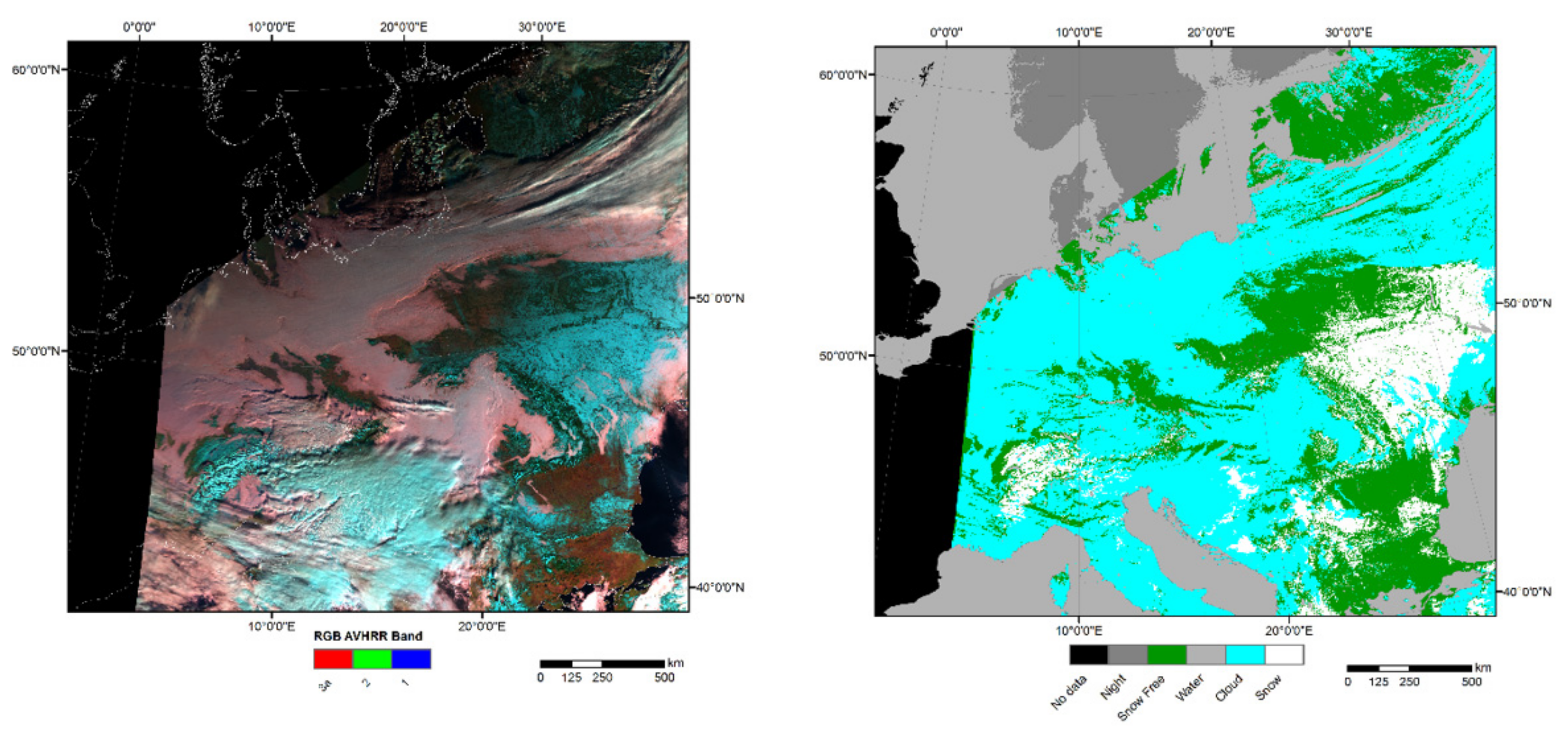In addition to the described snow mask (Figure 13), the Level 2 snow product also contains a layer with the raw NDSI values and an accuracy layer in which questionable pixels are marked.

In the Level 3 snow product, the individual orbits are merged into a daily snow product for each of the four tiles covering the LAEA region (Section 3.9); all L3 snow products retain this projection and tiling scheme. When joining the orbits, priority is given according to the assigned quality flags. The aim is to minimize the influence of clouds as well as questionable classifications (descending prioritization: night or missing data, high cloud probability, water detection, bad illumination conditions, high brightness temperature, high SWIR reflectance, and low VIS reflectance). In addition to the daily product, an 8-day composite is formed in order to further minimize the influence of clouds. Both Level 3 products enable good validation with the MODIS snow products [73], which are also based on the NDSI (Figure 14).

4.3. Fire Hotspots

Consistent and accurate mapping of wildfires is important to understand the impact of fires on global change. A database of hotspots in Europe for many decades can also be used in other research fields like forest management, wildlife management, or atmospheric chemistry.

Within the TIMELINE project a fully automatic instantaneous fire hotspot detection processor based on AVHRR imagery was developed [74]. The following section outlines the hotspot detection based on L2 AVHRR data elaborately described in [74]. We note here that the detection of fires that were active during the overpass of the satellite was performed directly in orbit geometry (L2) in order to avoid the loss of possible fire hotspots caused by the interpolation processes that are required during map projection (cf. Section 3.9).

Data from AVHRR channel 3B (mid infrared MIR, wavelength λ = 3.55 µm to 3.93 µm) and channel 4 (thermal infrared TIR, λ = 10.5 µm to 11.5 µm (AVHRR-1) or λ = 10.3 µm to 11.3 µm (AVHRR-2 and AVHRR-3)) are used for the fire detection procedure. The developed algorithm is intended to map as many active fires as possible; however, due to sensitivity limitations of AVHRR, it mainly detects very hot fires (i.e., covering only a subpixel portion of an AVHRR pixel), or larger, and cooler fires covering larger areas.

The fire hotspots detection algorithm uses the results of the cloud and water mapping procedure described in Section 3.6 in order to exclude those pixels from further processing. Urban areas and especially desert areas might show temperature values (up to 340 K) which are over the saturation temperature of the AVHRR sensor (322 to 331 K). Consequently, these areas had to be excluded prior to the execution of the core hotspot detection processor. Therefore, as sources for the exclusion masks, a LULC data set [75] and the global urban footprint (GUF) [76] were used. In addition, the fractional vegetation cover (FVC) was calculated from the AVHRR imagery and all areas with an FVC < 0.1 were excluded. As the hotspot detection processor could falsely interpret sun glint as high temperature objects, possible sun glint occurrence areas were pre-calculated and excluded from subsequent processing. Details about the exclusion masks are described in [74].

The fire hotspot detection algorithm itself performs several steps. First, possible fires, i.e., hotspot candidates, are selected. The hotspot detection processor distinguishes between daytime and nighttime acquisitions and performs three different runs with different thresholds, resulting in three different fire probability levels (the details of the thresholds are given in [74]). Next, within a contextual approach around each fire candidate a window of 5 × 5 pixels is created, which is increased up to 21 × 21 pixels until at least 25% of the background pixels in the window are valid. If a sufficient number of valid background pixels is identified, a series of statistics is computed. These statistics include the mean and the mean absolute deviation of the difference of the brightness temperature of channel 3 and channel 4 (for daytime and nighttime) and the one of channel 4 (daytime only). Finally, a fire candidate pixel is classified as a fire if the difference of the channel 3 and channel 4 brightness temperature is higher than that of the background plus a certain threshold and if the brightness temperature in channel 4 is higher than that of the background plus the mean absolute standard deviation of the background of channel 4. The last condition is only true for daytime imagery. The resulting fire pixels are assigned to the quality levels low, medium and high according to their neighborhood to water, clouds, bare land and urban area.

The results of the developed fire hotspot detection algorithm were validated (1) with a simulated data set (under 60 different conditions with varying fire size, fire temperature and background temperature) and (2) with real AVHRR imagery. For the second validation the following reference data were used: (a) MODIS hotspot data, (b) visually confirmed MODIS hotspot data, (c) EFFIS Fire-News data, (d) data from the Copernicus Emergency Management Service, and (e) data from the fire database of Piedmont. The tests were performed for fires in the following regions: Portugal, Sicily, Piedmont, Greece, and Sweden (Figure 15). The validation results are described in detail in [74]. The developed hotspot detection processor is an enhanced version of the hotspot detection algorithm described by Giglio et al. [77]. Both the original [77] and the enhanced processor developed in TIMELINE were tested against the same reference data. The great improvement of the new algorithm compared with the original one is a more than threefold reduction in the number of false positives, while keeping the number of true positives stable. The number of false negatives is very similar for both algorithms. The exact details of the conditions and parameters for the fire hotspot detection are described in [74].

The results of the fire hotspot detection (L2 hotspot product) were then transformed to the LAEA-ETRS89 map projection. Thereby, the point coordinate of each individual hotspot was transformed from latitude/longitude to LAEA-ETRS89 map projection. No interpolation was applied and all hotspots were preserved and then stored as an L3 hotspot product. The final result is an L3 fire hotspots detection product, which is currently being evaluated as to the temporal evolution of fires in Europe during the last four decades.

4.4. Burnt Area Mapping

In addition to the identification of fires active during a satellite overpass, a second TIMELINE algorithm determines burnt areas from AVHRR time series. A general problem with Earth Observation using optical remote sensing sensors is obscuration by clouds. In cloudy conditions, actively burning fires (hotspots) cannot be detected. However, if the burnt area covers a certain size, it can be detected up to several weeks after the fire ceased. The developed burnt area algorithm is described in detail in [78]. The following section gives a summary of this algorithm. The developed burnt area mapping algorithm is based on AVHRR data from channel 1 (red band, λ = 0.58 µm to 0.68 µm) and channel 2 (NIR band, λ = 0.725 µm to 1.1 µm). Only daytime imagery can be used for burnt area mapping.

The burnt area mapping algorithm performs a time series analysis. Required inputs are (1) an AVHRR scene acquired during or after the fire (called post-fire), (2) a series of AVHRR acquisitions of the 30 days prior to the fire event (called pre-fire), and (3) a LULC data set [75]. The current version of the burnt area mapping algorithm uses surface reflectance data (in LAEA-ETRS89 projection) as input, i.e., only the pixels per scene that were acquired under clear sky conditions and corrected for atmospheric effects (cf. Section 3.7 and Section 3.8). First, water-covered areas are excluded based on the LULC data set. Second, a histogram match of all AVHRR scenes is performed. Third, a clear sky pre-fire mosaic based on the pre-fire AVHRR scenes of the 30 days prior to the fire event is generated by using the most recent pre-fire image as base and step by step filling all missing pixels (originally cloudy) with valid information from the previously available AVHRR image. Fourth, a series of indices is calculated: (a) The NDVI of the pre-fire mosaic, (b) the NDVI of the post-fire scene, (c) the difference of the post-fire NDVI and the pre-fire NDVI, and (d) the burnt area index (BAI) [79] of the post-fire scene. Next, an automated thresholding of the BAI post-fire result is performed based on the OTSU method [80] and the maximum entropy method [81]. Finally, the detected burnt area pixels are assigned to different probability levels according to a series of criteria, such as (a) neighborhood to non-valid pixels (cloudy or covered by water), (b) confirmation of the burnt area by a decrease in NDVI when comparing with pre-fire information, and (c) type of LULC class where the burnt area was detected. The details of the indices calculation and criteria setting are given in [78].

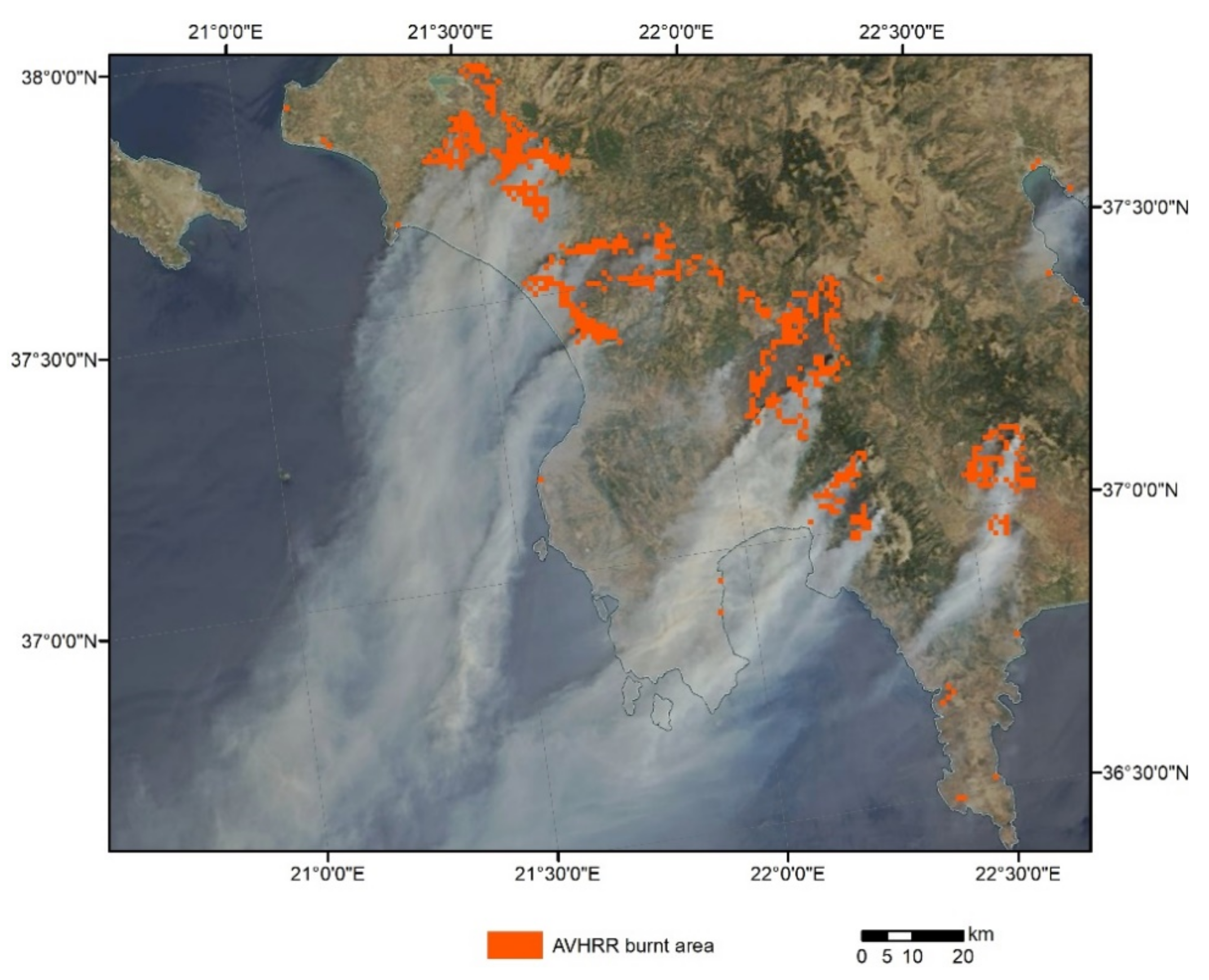
The first version of the burnt area mapping algorithm (cf. [78]) was validated with the MODIS burnt area product MCD64 [82] as well as with cloud-free data from the Landsat-7 Enhanced Thematic Mapper Plus (ETM+). Validation of the burnt area mapping results was carried out at four test sites in Sicily, Greece (Figure 16), Croatia and Hungary. A count-based accuracy assessment showed an average detection rate of 86%, with 14% overestimation and 7% underestimation. Burnt area information derived from Landsat-7 was additionally used to assess the accuracy of (1) the AVHRR-based classification and (2) the MCD64 itself. The details of the validation results are given in [78].

Currently, the TIMELINE burnt area algorithm is being further developed with newly available surface reflectance data as input instead of the top-of-the-atmosphere L1b data used for the first version of the algorithm presented in [78].

4.5. Land Surface Temperature

Land Surface Temperature (LST) plays a crucial role in the global heat balance. Therefore, monitoring changes in LST over large areas and for long time periods is important for tracing the impact of changing climatic conditions on our environment.

The TIMELINE LST product is derived from the brightness temperatures of AVHRR channels 4 and 5. As opposed to the products derived from channels 1, 2, and 3, atmospheric correction is performed with an extension of the Split Window Algorithm by Becker & Li [83] for AVHRR 2 and 3 and an extension of the Mono Window Algorithm by Qin et al [84] for AVHRR 1. Frey et al. [85] extended these algorithms with a different set of coefficients for daytime and nighttime, each AVHRR sensor, sensor view angle class, Total Columnar Water Vapor (TCWV) class and LST class. The different spectral response curves of the AVHRR sensors as well as geometry effects, atmospheric conditions and AVHRR specific inconsistencies at different temperature levels are taken into account. A detailed description of the coefficients’ derivation can be found in [85].

Deriving LST via remote sensing is complicated by the emissivity of the surface, which describes the effectiveness of the surface in emitting energy as thermal radiation proportionally to a perfect black body. The emissivity of the surface cannot be measured directly from space, but has to be derived from vegetation and soil properties. For the TIMELINE LST product the vegetation cover method by Caselles et al. [86] is used, which combines the spectral information known for different land cover types with the seasonal fluctuation of the vegetation cover, represented by the NDVI. The latter is calculated from the AVHRR channels 1 and 2 of the respective scene, which restricts the TIMELINE LST product for the moment to daytime scenes. However, it is planned to expand the LST product to nighttime LST using the TIMELINE L3 NDVI product as input.

While the Level 2 product contains the LST of the respective AVHRR scene in orbit projection, the Level 3 product consists of daily, 10-days and monthly composites of LST projected to the LAEA-ETRS89 map projection, as described in Section 3.9. The composites contain the respective maximum, minimum, median and mean LST and their corresponding observation time expressed in true solar time. During the calculation of Level 2 LST a quality and an uncertainty layer are produced. The uncertainty value is the root of the sum of the squared uncertainties from the atmospheric correction and the calibration as well as the uncertainties due to measuring noise in the AVHRR thermal channels and geolocation errors. The quality flags indicate the quality of the emissivity estimation, the atmospheric correction and the input data used. With the Level 3 product the parameters slope, sensor view angle and snow cover are included in the quality layer. Furthermore, a statistical outlier filtering is applied. 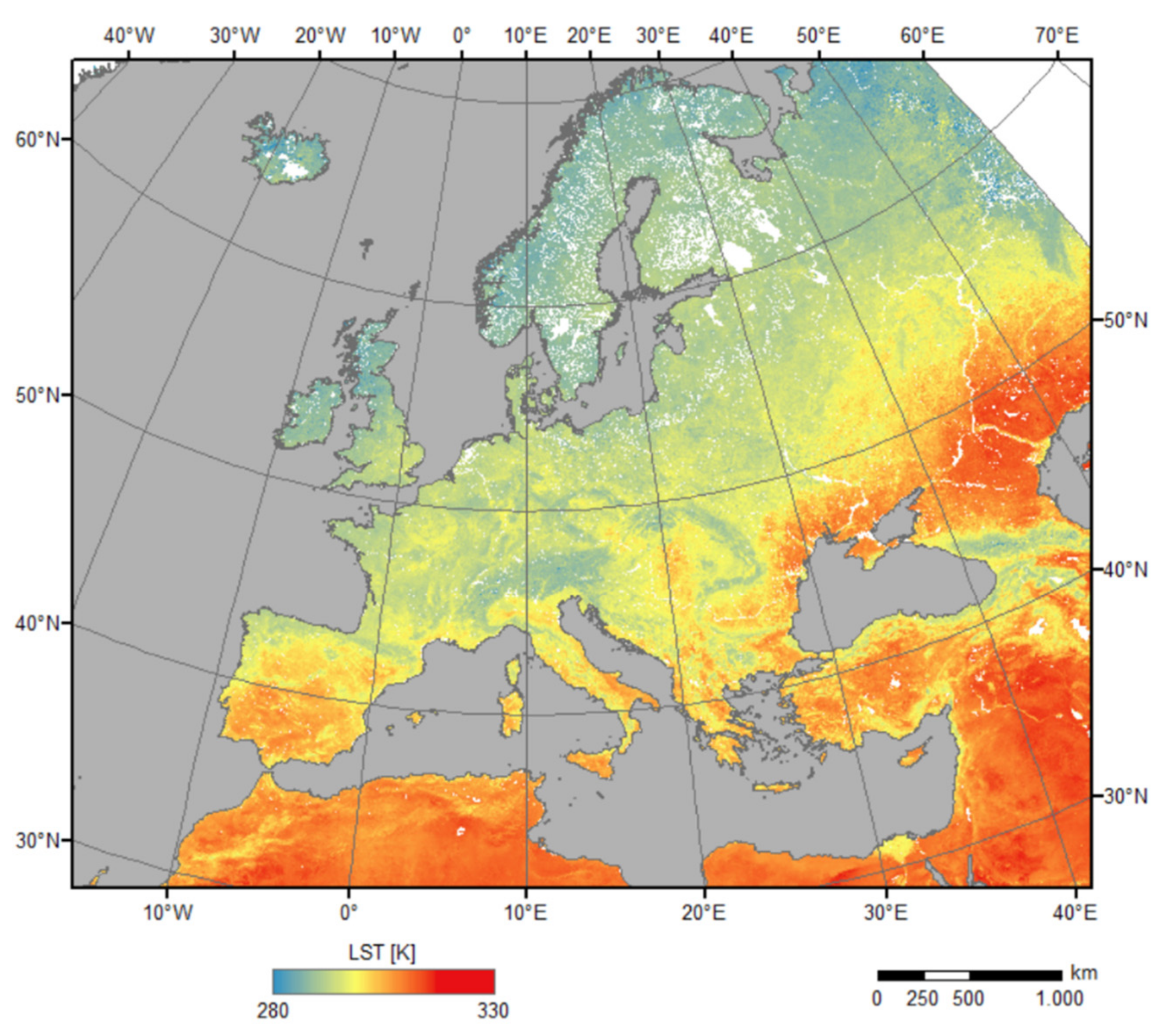Figure 17 shows the mean LST in August taken from the TIMELINE L3 LST product.

TIMELINE LST was validated along with the retrieval of the Split Window or Mono Window Algorithm coefficients by [85]. Their radiance-based validation resulted in MADs (Median Absolute Deviation) better than 1 K. Subsequent comparison to MODIS LST showed errors smaller than 2 K.

The different observation times of the NOAA satellites and orbit drift naturally constitute challenges when generating a multi-decadal LST time series since the variation of LST over the day is quite high. The TIMELINE LST time series at observation time can serve as valuable input for assimilation routines and climate models. Methods for daytime normalization for AVHRR use either the correlation between sun zenith angle and LST anomalies or trends [14,15,87], or try to model the diurnal cycle of LST [88,89]. Pixel-based methods often require large parts of the time series to get a representative range of observation times, which eliminates not only spurious, but also real trends. More general methods often rely on external data sources, which introduces new inconsistencies and uncertainties. The correction of orbit drift and daytime normalization for the thermal TIMELINE products is still under investigation. However, the unique collection of the TIMELINE vegetation and thermal products acquired under similar conditions offers the opportunity to develop the orbit drift and observation time correction not only for AVHRR, but also in general. First attempts to create a consistent and daytime normalized LST time series at three representative sites showed promising results. However, more general models are needed to be applicable to the whole TIMELINE study area. A TIMELINE Level 3b LST product is planned, which will be based on the quality assured TIMELINE LST Level 3 product. It will contain composites of daytime normalized LST with its associated uncertainties.

4.6. Sea Surface Temperature

Sea surface temperature (SST) is an important climate change indicator. Overall SST increased during the last century, but the changes also vary regionally [90]. These changes in SST affect the marine ecosystem in many ways and need to be monitored closely.

The sea surface can be seen as an idealized land surface as to spectral homogeneity. Therefore, SST can be estimated from the brightness temperatures of AVHRR channels 4 and 5 with the algorithms described in Section 4.5, assuming a constant emissivity value, which is taken from [91]. The constant emissivity allows estimation of nighttime SST without any additional auxiliary data. While the Becker & Li [83] split window algorithm was originally designed to estimate SST, the Qin et al. [84] mono window algorithm was developed to estimate LST from Landsat TM data. Its suitability for SST is still under investigation. Analogue to LST the Level 2 product contains SST in orbit projection and the Level 3 products contain projected daily, 10-day, and monthly composites. Daytime normalization is not a critical issue for SST, since the diurnal variations of SST are quite low. This means that the Level 3 product is ready to use for the time series analysis of SST. 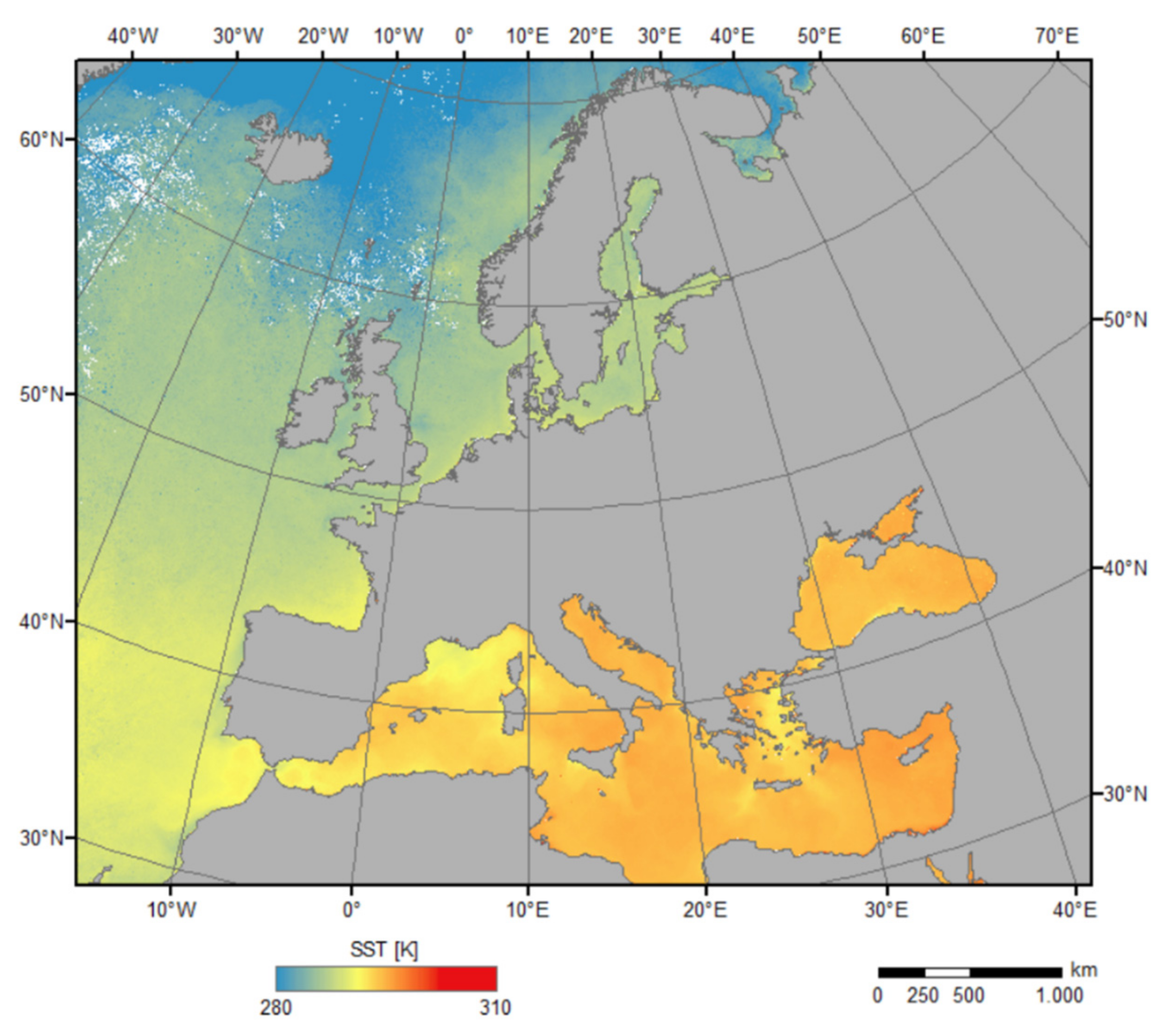Figure 18 shows the mean SST in July 2007 taken from the TIMELINE Level 3 SST product.

The TIMELINE SST was validated for the year 2009 for NOAA-17, -18 and -19 with Ships4SST radiometer measurements [92] and buoy measurements from the NOAA Global Drifter Array [93]. As expected, the accordance between TIMELINE SST and in situ measurements was better than observed during the TIMELINE LST validation: An RMSE of 0.87 K and a correlation of 0.99 was reached. This can be explained by the low temporal and spatial variability compared to LST. Opposed to LST, a dependence of the error on the SST level was not observed. Further validations of SST are planned. Since the uncertainties due to emissivity are missing and the TIMELINE SST is much more spatially and temporally invariant than LST, its validation can reveal new insights and a clearer picture of the Split Window or Mono Window Algorithm used to derive TIMELINE LST and SST.

4.7. Cloud Properties

Clouds are an important climate variable as they largely influence the Earth radiation balance and the hydrological cycle. The method applied in TIMELINE for cloud masking [43] also allows the retrieval of cloud properties and, as new feature with the probabilistic approach, their uncertainties (a prerequisite, e.g., for data assimilation into numerical models). The original APOLLO cloud property retrieval as outlined in Stephens [94] has been improved by exploiting the contrast between one non-absorbing and one absorbing channel for inferring optical depth and cloud droplet effective radius [95,96], separately for purely liquid phase clouds and for ice clouds. Cloud phase discrimination then yields the final value for optical depth and cloud droplet effective radius through representative weighting following the probabilistic approach. Once cloud optical depth, cloud droplet effective radius, and liquid phase fraction are determined, cloud top temperature and cloud water path can be calculated by inverting channel 5 for cloudy and clear radiances. Cloud water path can then be expressed as a function of optical depth and cloud droplet effective radius as well as extinction efficiency (set to a value of 2 for spherical liquid phase cloud droplets, and for ice clouds determined by the effective radius and the assumed crystal shape). Cloud properties in TIMELINE are provided as L2 products (single orbits) and as gridded L3 products. L3 products are offered at three spatial resolutions (10, 50, 100 km) and three temporal resolutions (daily, decadal = 10 days, monthly). Since clouds in the Earth atmosphere change very fast (within minutes) in their extent and properties, TIMELINE provides two types of gridded data which preserve the observation time. The classical L3 products (separate for data from each NOAA platform) contain an average local time stamp, and an L3b product (monthly, 10 km resolution) aggregates cloud properties of one month from all platforms in hourly local time slots.

Figure 19 shows maps of cloud property variables for one sample L3b (monthly) tile for July 2001 for the local time slot 14:00–15:00. Four NOAA platforms observing in the morning, early and late afternoon contributed AVHRR measurements in that month. At least six valid daily observations are required to create an L3-product. While for cloud fractional cover all pixels contribute, only pixels with cloud probability above 25% are exploited for cloud properties retrieval. We observe that cloud optical depth shows its maxima where cloud top temperature is lowest (highest-reaching clouds). For highest cloud optical depth, we also see maxima of cloud droplet effective radius and cloud water path while cloud phase tends towards icing conditions. The cloud droplet effective radius has unrealistic values in areas of very low cloud fractional cover over ocean (i.e., the cloud masking was too far optimized to cloud-free confidence here). As one additionally provided variable, precipitation likelihood also has its maxima at areas with the highest cloud optical depth values.

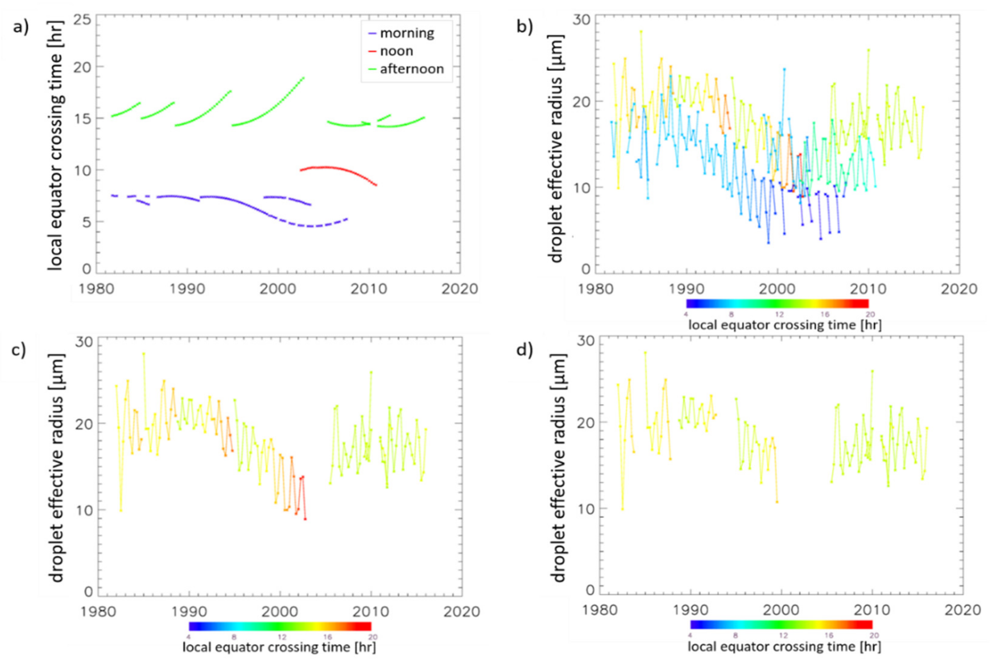
TIMELINE has the main goal of extracting climate data records, for which the AVHRR instrument series provides a promising long fundamental climate data record (almost 40 years). However, it also has a challenging inconsistency in the drifting and differing orbits of its individual instruments (cf. Section 3.1). Figure 20a shows an estimation of the equator crossing time for the different NOAA platforms calculated through extrapolation of the local time at nadir within the TIMELINE scenes (covering only Europe) to the equator (local equator crossing time LECT). Three major issues are obvious here: (1) Within one platform (connected line) the orbits are drifting, which leads to changing LECT (up to 5 h), (2) even for the same family of “morning” or “afternoon” satellites, the LECT is different, and (3) within one scene of 2048 pixels East–West, also the local time differs up to 1.5 hours. Given the fast change of clouds in the atmosphere, neglecting such changes in the daily observation time can spoil any climate data record retrieval.

Figure 20b–d show the example of a three-monthly averaged cloud droplet effective radius time series extracted from the NOAA-AVHRR record. The color coding indicates LECT. As shown in Figure 20b, morning hour observations (blue-ish colors) obviously tend to observe smaller droplets than afternoon observations (greenish to reddish), while an annual cycle is also visible with larger droplets in summer. A more homogeneous record can be expected by only analyzing observations of afternoon orbits, as in Figure 20c. However, this includes up to five hours of local time differences so that it needs to be questioned whether the decreasing trend visible between 1993 and 2003 is real or is due to the changing time of day. As a solution for such issues, TIMELINE supports the analysis of time series where a filtering for local time can be applied, as shown in Figure 20d where 14:00 < LECT < 16:00 reduces the suspected trend significantly. Such filtering can be done on the level of individual daily or monthly L3 products per platform (with the averaged LECT value for each file), or on the grid cell level per hour of the monthly averaged values in the L3b products. Such filtering will introduce gaps in a data record, but will improve its consistency with regard to the local observation time.

5. Discussion

High temporal resolution mapping of the Earth surface from space for more than 40 years creates an enormous wealth of data for the analysis of climate change effects on our environment. In order to be able to exploit these data, systematic and random errors in the raw data must be corrected. The associated archiving, processing, harmonizing and analyzing of AVHRR long-term time series poses a wide range of challenges.

As described in Section 3, several factors have to be taken into account concerning the analysis of AVHRR data. To ensure radiometric consistency, the satellite orbit drift and the channel calibration drift need to be corrected [4]. While the effect of the latter was reduced using SBAFs [21], orbit drift was accounted for by high and low gain harmonization, which reduced the NDVI differences of the respective platform to the mean NDVI of NOAA-19 at the validation sites roughly by a factor of 10 (cf. Section 3.3). Furthermore, atmospheric and BRDF corrections have been conducted in order to provide SDR data and to account for the varying observation times caused by orbit drift, and hence to further increase the radiometric quality of the AVHRR data. Nevertheless, variables derived from AVHRR data with a diurnal cycle like temperature, or rapidly changing variables like cloud properties, must still consider the temporal inconsistencies of the AVHRR sensors, making use of filtering or normalization methods in order to create meaningful data records (cf. Section 4.5, Section 4.6 and 4.7).

Further challenges regarding the geolocation of AVHRR have been met by developing a chip matching procedure and an orthorectification process (cf. Section 3.4). Scene-specific cloud and water masks ensure the exclusion of signals disturbing the land surface reflectance (cf. Section 3.6), and formatting the generated data sets according to a common standard format, extent, and projection ensure that the product suite is ready to use (cf. Section 3.9).

The development of a well-thought-out framework for big data processing (cf. Section 3.10) was another essential component for efficient AVHRR time series processing. Experience showed that the operation of archive tapes in streaming mode, i.e. loading data from the archive and caching them on the hardware platform used, is crucial. This buffering enables the stabilization of fluctuations in the staging process and ensures a continuous but flexible input data stream. This is a prerequisite for the second fundamental system requirement, its parallelization capability. The flexible scalability of the different processing workflows regarding their individually needed resources enabled us to employ a multi-decadal, continental scale data set. Furthermore, rigorous configuration control, including the versioning of software, inputs and products, needs to be implemented in such an endeavor to ensure traceability, compatibility and the subsequent use of products.

Quantitative studies of Earth’s surface dynamics can only be realized if the input data have been appropriately corrected for disturbing effects [91,97,98]. Trends caused by sensor degradation need to be avoided [3]. Appropriate correction procedures were considered within TIMELINE. Nevertheless, the correction of orbital drift and sensor changes is always based on vicarious calibration and modeling approaches, usually with residual errors being unaccounted for. Hence, instabilities might still remain that mitigate or enhance artificial trends [99]. In this context, we emphasize the importance of additional qualitative information and quality control provided for all products developed within the TIMELINE project in order to better evaluate uncertainties in the results (cf. Section 4).

Further issues like undetected outliers or data gaps (spatial and temporal) may influence the analysis of TIMELINE products. As shown in Figure 21, TIMELINE AVHRR data is not available at the same frequency for its entire lifetime, with periods of only a few scenes per day over Europe (e.g., in 1981–1987) or complete data gaps (e.g., June 2014 or August and September 2018). Time series analysis relies on the temporal signal at the pixel level [100], and for certain analysis like annual peak phenology equally spaced data is a prerequisite. Data gaps should therefore be considered or made visible in further time series analyses. But also phases of unusual data abundance, like in 2010, need to be critically considered, such as when inspecting short-life events like hotspots or cloud formation that rely on single scenes rather than on composites.

The AVHRR observations are a unique remote sensing data set in terms of temporal coverage and of temporal and spatial resolution. This exclusivity makes it valuable on the one hand, but on the other hand it limits the comparison to data from other sources, which is an important pillar of validation of geospatial products. Remote sensing data suitable for a sensor-to-sensor comparison only became available from the year 2000 onward with the launch of MODIS Terra. Although Landsat data has been available since the early 1980s, a comparison between AVHRR and Landsat data is challenging due to the different spatial (Landsat: 30 m, AVHRR: 1.1 km) and temporal resolutions (Landsat: 16 days, and no continuous acquisitions, AVHRR: several times daily). For the validation of the reflective channels, pseudo-invariant desert sites (e.g., for TIMELINE the CEOS PICS Algeria3 and Lybia4) can be used under the assumption that the target reflectance is indeed constant. Bottom-of-atmosphere-reflectance reference measurements from instrumented sites like La Crau, France, have been available since ~2000 (CNES, pers. communication), and due to the large footprint of AVHRR they have to be carefully integrated in the validation process. For the validation of higher-level products, additional sites like DEMMIN can provide thematic data products such as LAI derived from campaigns or continuous measurements. The lack of in situ measurements and concurrent remote sensing products for the earlier period of AVHRR leads to uneven validation of the AVHRR time series. Should comparable AVHRR products (with the same spatial resolution and similar processing) be available from other data providers, we will consider them for direct comparison in the TIMELINE validation process.

Overall, we have succeeded in creating a harmonized time series from the AVHRR data, knowing the possibilities but also the limitations of this unique data set and its further products.

6. Conclusions

We have outlined all of the steps necessary to create a harmonized time series of daily NOAA AVHRR observation data over four decades. This unique data set serves as input to investigate long term impacts of climate change on our environment. The effort of data harmonization was carried out as part of the TIMELINE project, which aims at monitoring global change related processes in Europe and North Africa. Only by providing a harmonized time series of Earth Observation data free of systematic errors and artefacts is it possible to perform sound analyses related to the extent of changes in land surface dynamics due to climate change. Within TIMELINE the fully automated processing chain produces more than 15 different AVHRR geospatial products from L1 to L3. Up to now, 500 TB of data have been processed. Constant monitoring of the data quality and regular validation of the different products ensures a deep knowledge of the quality of the TIMELINE products. Accordingly, these products are also intended to serve as input to climate models, and the results of trend analyses of the AVHRR time series should also provide quantitative evidence of climate change impacts.

In the near future, further L3b products will be derived from the data pool of TIMELINE L3 land, sea, and atmosphere products. Free and open dissemination of the TIMELINE products is foreseen after final quality control.

We see great potential to adapt the TIMELINE processing framework to further EO time series data and to continue with other sensors with higher spatial and spectral resolution (e.g., Sentinel-3).