Article

High-Resolution Mining-Induced Geo-Hazard Mapping Using Random Forest: A Case Study of Liaojiaping Orefield, Central China

1
Key Laboratory of Digital Land and Resources, East China University of Technology, Nanchang 330013, China
2
Faculty of Earth Sciences, East China University of Technology, Nanchang 330013, China
3
Key Laboratory of Natural Resources Monitoring and Supervision in Southern Hilly Region, Ministry of Natural Resources, Changsha 430103, China
4
Department of Remote Sensing and GIS, Faculty of Geography, University of Tehran, Tehran 1417853933, Iran
*
Author to whom correspondence should be addressed.
Remote Sens. 2021, 13(18), 3638; https://doi.org/10.3390/rs13183638
Submission received: 26 July 2021 / Revised: 6 September 2021 / Accepted: 7 September 2021 / Published: 11 September 2021

Abstract

:
Mining-induced geo-hazard mapping (MGM) is a critical step for reducing and avoiding tremendous losses of human life, mine production, and property that are caused by ore mining. Due to the restriction of the survey techniques and data sources, high-resolution MGM remains a big challenge. To overcome this problem, in this research, such an MGM was conducted using detailed geological exploration and topographic survey data as well as Gaofen-1 satellite imagery as multi-source geoscience datasets and machine learning technique taking Liaojiaping Orefield, Central China as an example. First, using Gaofen-1 panchromatic and multispectral (PMS) sensor data and Random Forest (RF) non-parametric ensemble classifier, a seven-class land cover map was generated for the study area with an overall accuracy (OA) and Kappa coefficient (KC) of 99.69% and 98.37%, respectively. Next, several environmental drivers including land cover, topography (aspect and slope), lithology, distance from fault, elevation difference between surface and underground excavation, and the difference of spectral information from PMS multispectral data of different years were integrated as predictors to construct an RF-based MGM model. The constructed model showed an excellent prediction performance, with an OA of 98.53%, KC of 97.06%, and AUC of 0.998, and the 85.60% of the observed geo-disaster that have occurred in the predicted high susceptibility class (encompassing 2.82% of the study area). The results suggested that the changes in environmental factors in the high susceptibility areas can be used as indicators for monitoring and early-warning of the geo-disaster occurrence.

1. Introduction

Mining-induced geo-disasters (MG) are a type of disaster related to geological processes induced by natural and/or man-made factors [1,2]. These disasters, which include debris flow, landslide, collapse, ground fissure, and subsidence, are usually caused by intensive mining activities with tremendous damage to the natural and man-made environment, such as water bodies, farmlands, roads, and pipelines. More importantly, mining-induced disasters lead to mining accidents and losses of human life and property and even reduce the sustainability and stability of development among human beings, resources, and the environment. Hence, some useful prevention measures and technology of MG must be proposed [3,4,5]. Mining-induced geo-hazard mapping (MGM) based on determining the relative probability of geo-disaster occurrence is essential for real-time monitoring and prediction of the spatial patterns of geological disasters and subsequently protection of the ecological resources and human health in the mining areas [6,7].
Qualitative or semi-quantitative estimation of the occurrence possibility is considered a common procedure for evaluating geo-disaster susceptibility, especially for individual disasters. This can be implemented by studying the mechanism of geo-disaster occurrences, identifying triggering factors, and then using these factors to simulate the deformation progress of the related geological bodies, especially for the single landslide triggered by rainfall or earthquake [8,9,10,11,12]. Various geo-disasters may occur concurrently by the same type of environmental factors, such as rainfall, geological structures, and excavation activity. Moreover, trigger factors caused by geo-disasters should be used for predicting and evaluating geo-disaster susceptibility. The characteristics of geological structures are one of the important factors in the field of MGM. In this regard, Wang et al. [13] developed a disaster-area prediction model that is based on analyzing the correlation of geo-disaster with mining-induced activity, lithology, and geological structure. In another study, Segoni et al. [14] performed a landslide susceptibility mapping approach using various geological data including structural, lithology, chronologic, genetic units, and paleogeography. These triggering and triggered factors, as well as the geological and geographical conditions and environmental factors, can be obtained from field-based disaster investigation, geological survey, and remote sensing (RS), taking advantage of the earth observation satellite data, geographic information system (GIS) technique, and machine learning modeling [15].
In order to quantitatively conduct MGM, it is necessary to first consider all causes of previous events and accordingly analyze the association between disasters with different environmental drivers using data-driven methods in the GIS platform [16,17,18,19]. In the literature, various multi-source geospatial data, i.e., topographic features, geological information, rainfall conditions, and vegetation indexes (VIs) from field survey and satellite imagery were used as environmental predictive factors for MGM using powerful data-driven methods, such as support vector machine (SVM) [20], logistic regression (LR) [21], artificial neural networks (ANN) [22], random forest (RF) [23], decision tree (DT) [24], weights of evidence (WofE) [20], frequency ratio (FR) [25], analytic hierarchy process (AHP), and linear combination (LC) [26,27]. Overall, a wide variety of approaches have been used for MGM, among which supervised machine learning algorithms have shown high efficiency and reliability. In recent years, these methods have been successfully applied in the field of geoscience, especially for mineral prospectivity mapping (MPM) and MGM [15,28,29,30,31,32,33,34,35,36,37,38]. MG occurs suddenly within/around mining areas with the characteristic of small scale, high density, and frequency. Due to the vital need for more detailed mining activity and geological exploration data, the implementation of MGM is associated with some restrictions [8,39]. Despite numerous studies in this field, due to the restriction of the survey techniques and data sources, MGM with high-resolution remains a major challenge.
Preparation of land cover map is a preliminary to analyzing physiognomy characteristics and evaluating land resources, and it also definitely facilitates the prediction and evaluation of MG. Under normal circumstances, different land cover types indicate the different levels of human activities as the triggering factors of MG. Utilizing multispectral and multi-temporal RS datasets is a momentous approach to mining geospatial information. For example, a great number of researchers obtain the land use/cover maps based on RS image classification techniques by taking advantage of the capabilities of supervised machine learning methods (e, g., RF, SVM, ANN, and LR) [40,41,42].
Nowadays, thanks to the development of high-spatial- and spectral-resolution RS technology, it has become feasible to extract more precise and comprehensive geospatial information. In the same context, Youssef [43] generated predictive geo-disaster drivers by integrating 15 m resolution satellite imagery and 10 m contour maps to obtain the landslide susceptibility indices. Pachuau [44] identified the areas susceptible to landslide occurrence with a variety of high spatial resolution satellite datasets, i.e., Quick Bird, IRS, and Cartosat-I imagery. Arabameri et al. [45] used RS datasets with different spatial resolutions to assess landslide susceptibility based on combined FR and RF approaches. In their study, the sample data were collected from various resources, such as extensive field surveys, historical records, aerial photo interpretation, and high-spatial-resolution Google Earth images.
The Liaojiaping Orefield, which is located in Hunan province, Central China, is an important part of the gold (Au) and antimony-tungsten (Sb-W) polymetallic metallogenic belt in the southern branch of the middle Xuefeng Arcuate Tectonic Belt (XATB). The main deposits hosted in this orefield have been indiscriminately mined for decades. Coupled with the complex geological and structural setting of the mining areas, this has led to the frequent occurrence of different MGs such as landslip, collapse, land subsidence, and fissure. It should be noted that these MGs directly restrict mine exploitation and pose serious threats to human life and property. In the absence of systemic research on susceptibility, these disasters are difficult to prevent. Accordingly, the main purpose of this study is to perform a high-resolution MGM in Liaojiaping Orefield based on multi-source high spatial resolution geo-environmental data using data-driven methods, taking the main environmental factors that are associated with MG into account.

2. Study Area and Materials

2.1. Geological Setting

Liaojiaping Orefield, covering an area of 41.25 km2 and located in the central Hunan province, China, is situated in the southern margin of the middle XATB, which is developed between the Dongting Basin and the Gui-Xiang subsidence belt in the Yangtze Block and consists of Northeastern Hunan fault-uprising belt and the Xuefeng thrust belt (Figure 1). The approximately EW- and NE-striking faults and the secondary anticlines with the NE direction axis in this tectonic setting form the basic structural framework of the orefield (Figure 2). These multi-phase geological structures intricately crisscross and lead to the dip and steep landform.
The fine clastic rocks intercalated with carbonate rocks that were deposited in the epicontinental rift basin environment from Lower Proterozoic to Upper Paleozoic Era and the carbonate rocks intercalated with clastic rocks in the epicontinental basin environment (later Paleozoic) form the stratigraphic assemblage of this region. The strata from Sinian to Devonian are well exposed in this orefield, and the Quaternary sediments are mainly deposited in the northwest corner (Figure 2 and Table 1). The outcrops of different strata have been experiencing various degrees of weathering and splintering; for example, the fine sandstone in the Upper Zhoujiaxi Formation of Lower Silurian presents a bead shape as a result of an intense spheroidal weathering process.

2.2. Geological Disasters

This orefield has been mined on and off for more than half a century. Early unauthorized and later wasteful mining activities led to a series of environmental problems in these mining areas, such as ground deformation, water, and soil pollution. The MG often occurring next to each other cause serious damage to human life and property, although the mining has been conducted in a more scientific and cautious way in the last decade. For example, the landslide that occurred in July 2018 caused one death and two injuries in one family in the Tianchelun mine of this orefield. This highlights the need for MGM using multi-source environmental factors that are related to the geological setting and mining activities.
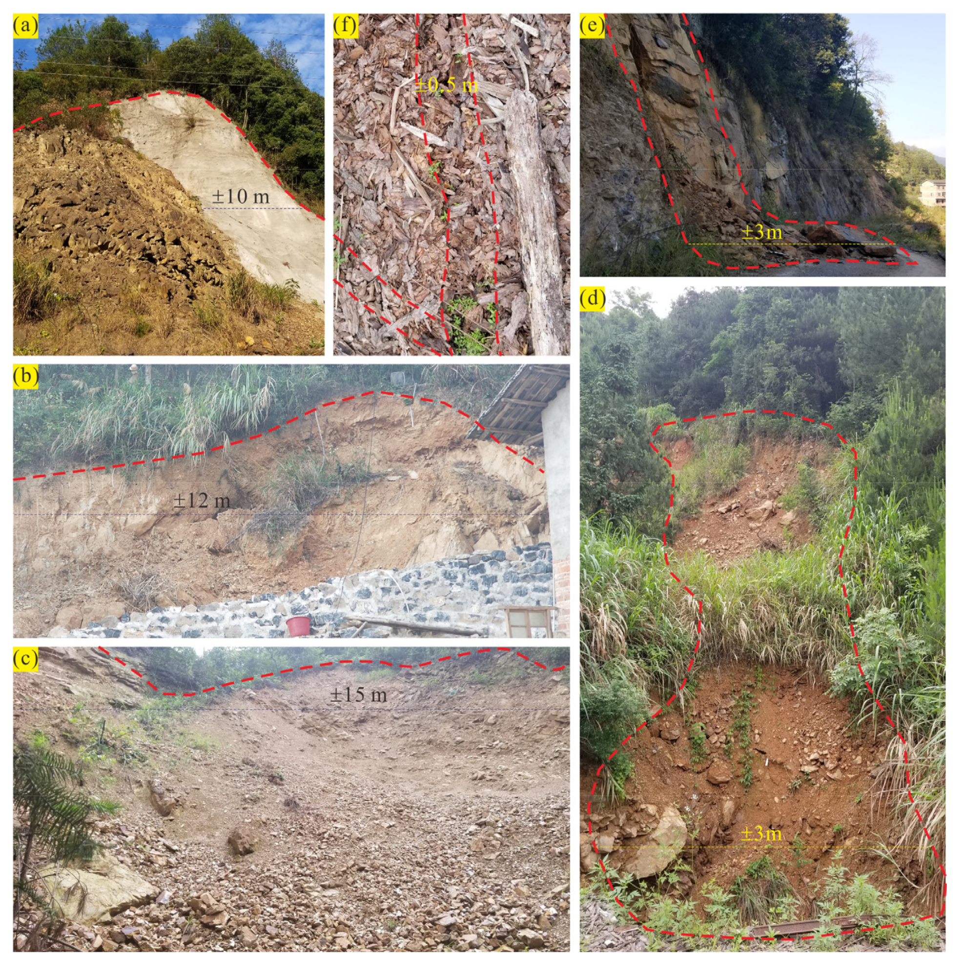
It took several months to investigate the MG that occurred in Liaojiaping Orefield, and the survey results showed that the landslide, collapse, land subsidence, and fissure erratically took place in this orefield, especially in case of heavy rainfall. The main characteristic of MG is that they usually occur at a different scale around mining and excavated areas. The difference in lithology and physical environment leads to different degrees of outcrop weathering, and in this circumstance, various MGs are triggered in these outcrop areas by various types and scales of human activities. The MGs that occurred (e.g., Figure 3) are mainly medium–small in size in the Liaojiaping Orefield. In this regard, the detached mass of landslides in Figure 3a,b is less than 1000 m3, the biggest collapsed area (Figure 3c) is no more than 500 m2, and other common collapsed areas (e.g., Figure 3d) are about 10 to 100 m2. Most of the collapsed blocks (e.g., Figure 3e) are only several m3, and the ground fissures are normally tens of centimeters in width and several meters in length (e.g., Figure 3f). Some of these MG are interconnected in terms of occurrence; e.g., the ground fissures above the mining areas always occur before the subsidence, and the places often affected by the collapse may concurrently produce landslides.

2.3. Multi-Source Geo-Environmental Data

The occurrences of MG in the Liaojiaping Orefield are often related to different factors including underground mining, geological structures, topographic features, near-surface excavation, and rock weathering. In addition to these factors, the land cover information and surface spectral characteristics can be also used for MGM. MG investigation, geological survey, mineral exploration, and RS are vital and common techniques that can provide all mentioned multi-source geo-environmental data necessary for MGM.
The dataset composed of the above factors is actually an integration of different variable layers that are rasterized into the same grid size, and the sample set, an important part of this grid dataset containing the target variable, is used for training the prediction model and its validation. The determination of features (for the whole dataset) and the target variable (for the sample set) plays an important role in the construction of the prediction model, and these variables, which are used as predictive factors [46,47], need to be explored by different methods, and their spatial autocorrelation must be reduced [48].
Three Au and two Sb-W deposits have been mined for more than 20 years in the study area. The data supporting this study can be sourced accordingly: (1) the detailed geological data acquired by continuous geological survey and exploration, i.e., the main stratigraphic units and faults presented in the geological map of the study area (Figure 2); (2) the exploration data from mining activities, such as tunnels and stopes implemented in the mining areas; (3) the topographic features such as aspect and slope values extracted from the high-precision topographic map on the scale of 1:5000; (4) the minor structures and the surface spectral characteristics (e.g., VIs) obtained and interpreted using high-resolution RS imagery, in this case, Gao Fen-1 (GF-1) satellite, which was launched on April 26, 2013 by CNSA (China National Space Administration) [49]. Two panchromatic and multispectral sensors (PMS) and four wide field-of-view (WFV) sensors are aboard the GF-1 satellite [50]. The present study took advantage of the PMS sensor data. The specifications of GF-1/PMS are presented in Table 2.

3. Methodology

The results of different statistic-based prediction models for MGM are quite different [51,52,53]. For a certain algorithm, it may achieve good prediction accuracy/performance in one case but perform poorly in another. The intrinsic structure of samples must be the decisive factor that causes this situation. In the same context, Kalantar et al. [54] and Qin et al. [37] have also pointed out that the determination of the sample dataset has a direct effect on the model prediction accuracy. Accordingly, to increase the generalizability of the predictive model, it is adequate to combine the classical and popular mathematical methods to construct a robust prediction model as long as the relevant dataset is well prepared.

3.1. GF-1 Image Processing

Band ratio operation, multispectral transformation, and image filtering are important techniques for image enhancement and extraction of spectral information of the ground objects after preprocessing, including ortho-rectification, radiometric calibration, and atmospheric correction [55]. For the GF-1 imagery, the spatial resolution of the multispectral bands can be improved to 2 m by fusing them with the panchromatic band so that it can meet the requirements of this study despite its low spectral resolution.

3.1.1. Band Ratio Operation

All kinds of VIs that can detect spatiotemporal patterns of vegetation can be used as an important factor for land cover classification [32]. Kaufman and Tanré [56] proposed a VI named soil-adjusted atmospherically resistant vegetation index (SARVI) based on the soil-adjusted vegetation index (SAVI) [57], which can be written as Equation (1),
S A R V I   =   1 + L B N I R ( 2 × B R E D B B L U E ) B N I R + ( 2 × B R E D B B L U E ) + L
where L is a constant that is used to reduce the soil effect as much as possible, and it is suggested to be set as 1; BNIR, BRED, and BBLUE are, respectively, the reflectance of the near-infrared (NIR), red, and blue bands. SARVI is suitable for the strongly vegetated areas from various satellite sensors, and it also can be employed for vegetation analysis based on Gaofen-1/PMS data.

3.1.2. Image Transformations

With the help of color-space conversions and principal component analysis (PCA), the spectral information can be enforced while the noise is reduced to a certain extent. Munsell HSV transformation, which converts a three-layer color space of red (R), green (G), and blue (B), known as RGB, into another three-layer color space, including hue (H), saturation (S), and value (V), known as HSV, facilitates the description and distinction of the color features of soil and rock [58]. The theoretical model of the Munsell HSV transformation is presented as follows:
H = { 0 R = G = B   60 × G B max R , G , B min R , G , B + 1 max R , G , B = R 60 × B R max R , G , B min R , G , B + 3 max R , G , B = G 60 × R G max R , G , B min R , G , B + 5 max R , G , B = B
S = max R , G , B min R , G , B max R , G , B               max R , G , B 0 0                                                                               max R , G , B = 0
V = max R , G , B
where R, G, and B are the reflectance values of the corresponding RGB combined band, H is a range from 0 to 360, and S and V range from 0 to 1.
PCA, which is also known as the Karhunen–Loeve (K–L) transform [59], is used to generate a new spectral space F from the original space X that consists of n samples with p dimensions. The dimensions p of the space X can be reduced to m using a linear transformation matrix A, which contains m multi-feature vectors. The first few principal components of the new space F usually contain the vast majority of the spectral information. This process can be described as Equation (5):
X = { x 11 x 21 x n 1 x 12 x 22 x n 2 x 1 p x 2 p x n p }            F = A X            F = { F 11 F 21 F n 1 F 12 F 22 F n 2 F 1 m F 2 m F n m }

3.1.3. Filtering

The purpose of image filtering is to highlight useful spatial information and depress the noise of a single image using various filters [60]. Convolutions and morphology are two common filtering methods. The convolution filtering intensity depends on the parameter-setting transform kernels, and the morphology filtering is generally used for effectively eliminating the noise in single bands.

3.2. RF-Based Classification Scheme and Prediction Model

3.2.1. RF Background

Developed by Breiman [61], RF is a type of ensemble learning algorithm and is constructed by multiple decision trees. A decision tree is a typical supervised learning approach that can be used to categorize or regress something based on the data we have [62]. Classification and regression trees (CART), which is an important dichotomy algorithm, are used to generate binary decision trees [63]. Determining the optimal feature for splitting and providing a condition to stop splitting are two critical processes of tree generation. For the classification tree, the Gini coefficient (Gini) is used to measure the impurity of the node splitting, and the feature with the minimum Gini can be used for splitting in the generation of decision trees (Equations (6) and (7)). For the regression tree, the minimum squared error (MSE) is used for splitting in decision tree generation [63]. The Gini criterion for node splitting is defined as:
G i n i   t = 1 p ( c k | t ) 2
where p ( c k | t ) is the probability of the class c k in the node t for a decision tree. There are two assemblies (DL and DR) corresponding to the left and right child nodes around the parent node, and the Gini after splitting can be defined as Equation (7):
G i n i D , A = D L D G i n i D L + D R D G i n i D R
In general, two random processes, namely bootstrap aggregating (bagging) [64] and stochastic subspace [65], are employed to construct RF. These two processes can help to ensure the accuracy of every tree and effectively avoid its overfitting. More details on the generation procedure of the RF are given in Qin et al. [37].

3.2.2. RF-Based Classifier

Each sample has only one single attribute class, both for the case of binary- and multi-class classification, i.e., all the attribute classes of the sample set are separately and exclusively present in one sample. For a sample set with n (1, 2…, n) attribute classes, it can be classified by n binary classifiers; every classifier has two classes, e.g., class 1 with classes (2, 3…, and n) or class 2 with classes (1, 3…, and n). In this way, one classifier can be learned for binary classification, while n classifiers will be learned for n-class problems from every training set.
The training and validation datasets are randomly determined using the bagging method from the sample dataset, and the ratio of these two sets is about 7 to 3 (i.e., 70% for training and 30% for validation). The RF-based classifier that was constructed based on multiple training sets will return a classification result based on the ratio of the votes provided by all the tree classifiers. In other words, the final attribute class is decided by the maximum of all the returned values (namely prediction probability) for every class.
The out-of-bag error (OBB error), F1 score, overall accuracy (OA), kappa coefficient (KC), and area under the receiver operating characteristic (ROC) curve are obtained from the generated confusion matrix based on the classification result and the validation dataset. These statistics can be used to evaluate the performance of the constructed classification and prediction model, and higher values indicate the higher prediction accuracy of the corresponding model [37,66]. The RF classifier can provide the relative importance of different features in the sample dataset, and this kind of importance value indicates their contribution to the decision tree, and thus, the correlation of every feature with the attribute class could be analyzed using other statistical methods.

3.3. Sample-Improved WofE Method

Weight of evidence (WofE), a multivariate statistical approach and fusion method based on probabilistic uncertainty and Bayes theorem, was developed for spatial correlation analysis and posterior probability prediction in mineral prospectivity mapping [67,68,69]. In the WofE analysis, the samples D (e.g., the MG occurrence) are used as training points, the geological factors that are related to the samples are used as evidential factors, and these themes should be generated as the grid file with a given unit cell size. In the study area T, the number of the grid cell is marked as N, and the prior probability of the sample occurrence is defined by Equation (8).
P D = N D N T
According to the theorem, the conditional probability of the sample occurrence with the appearance of evidential factor B j (j = 1, 2…, n) can be written as Equation (9):
P D | B j = P D B j P B j
The positive and negative weights of the sample occurrence are defined as Equation (10) and Equation (11):
W j + = ln P B j | D P B j | D ¯
W j = ln P B j ¯ | D P B j ¯ | D ¯
where the positive W j + and negative W j indicates that the occurrence of sample D is positively related to the evidence B j ; otherwise it has a negative correlation. In addition, this degree of correlation can be measured with the contrast (C), in which a larger positive C value means a greater positive correlation. For the evidence B j , its Cj is calculated by Equation (12):
C j = W j + W j
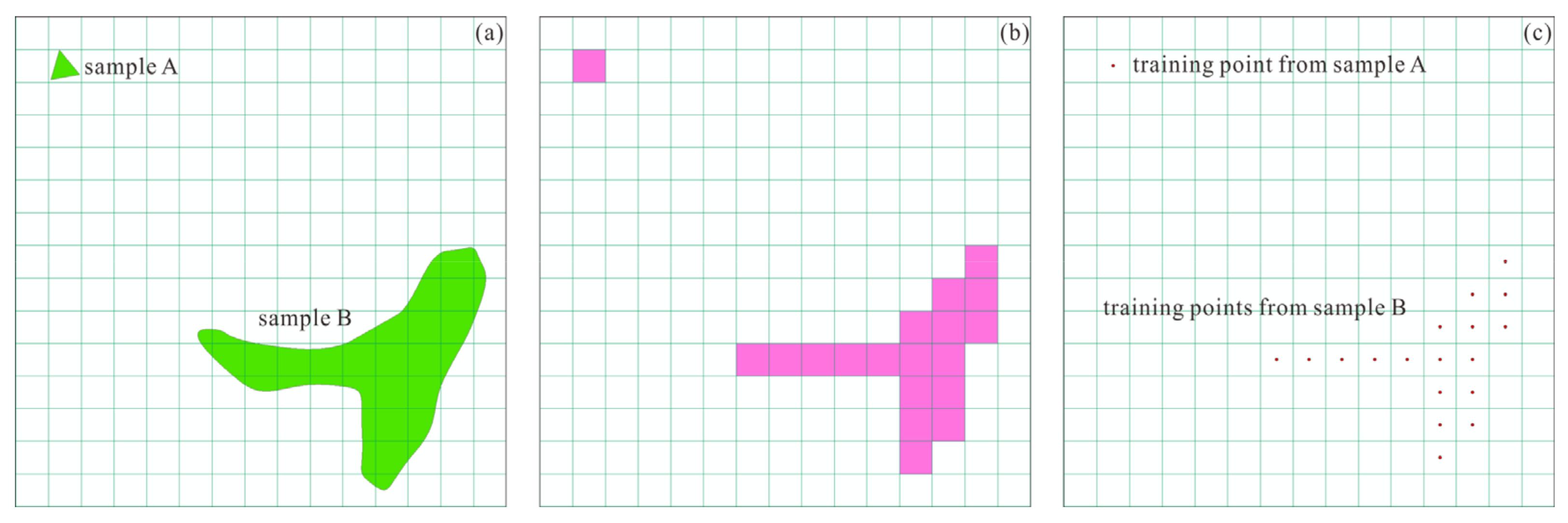
In conventional WofE analysis, all the samples are abstracted as the training points regardless of their spatial size. This process is able to reduce the number of sample occurrences and directly affects the correlation based on probability analysis between samples and evidential factors. Therefore, the areas of the sample occurrence are firstly identified and then grided into the same cell size as other factors of the study area. In this way, every sample area is converted into a certain number of training points for spatial correlation analysis (Figure 4). In addition, this approach is also suitable for improving samples to train machine-learning-based prediction models.

4. Results

4.1. Land Cover Mapping

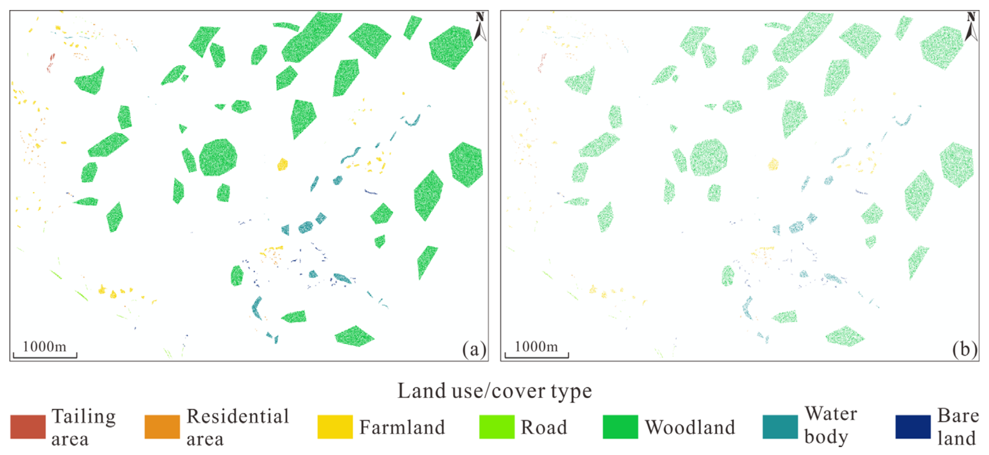
The study area encompasses 10,312,500 grid cells with a size of 2 × 2 m. In this study, RF classifier, as a non-parametric supervised machine learning algorithm, is employed for land cover mapping. The ground truth samples were determined based on GF-1/PMS (the year 2020) true-color image (TCI), composed of bands 3 (R), 2 (G), and 1 (B) (Table 2) based on the field disaster and land cover survey. The ground truth samples were randomly divided into two sets, i.e., training and validation sets, with a 7 to 3 ratio. Figure 5 shows the different ground truth land cover classes in the training and validation sets. As shown in Table 3, the training and validation sets occupy about 9.58% of the entire study area.
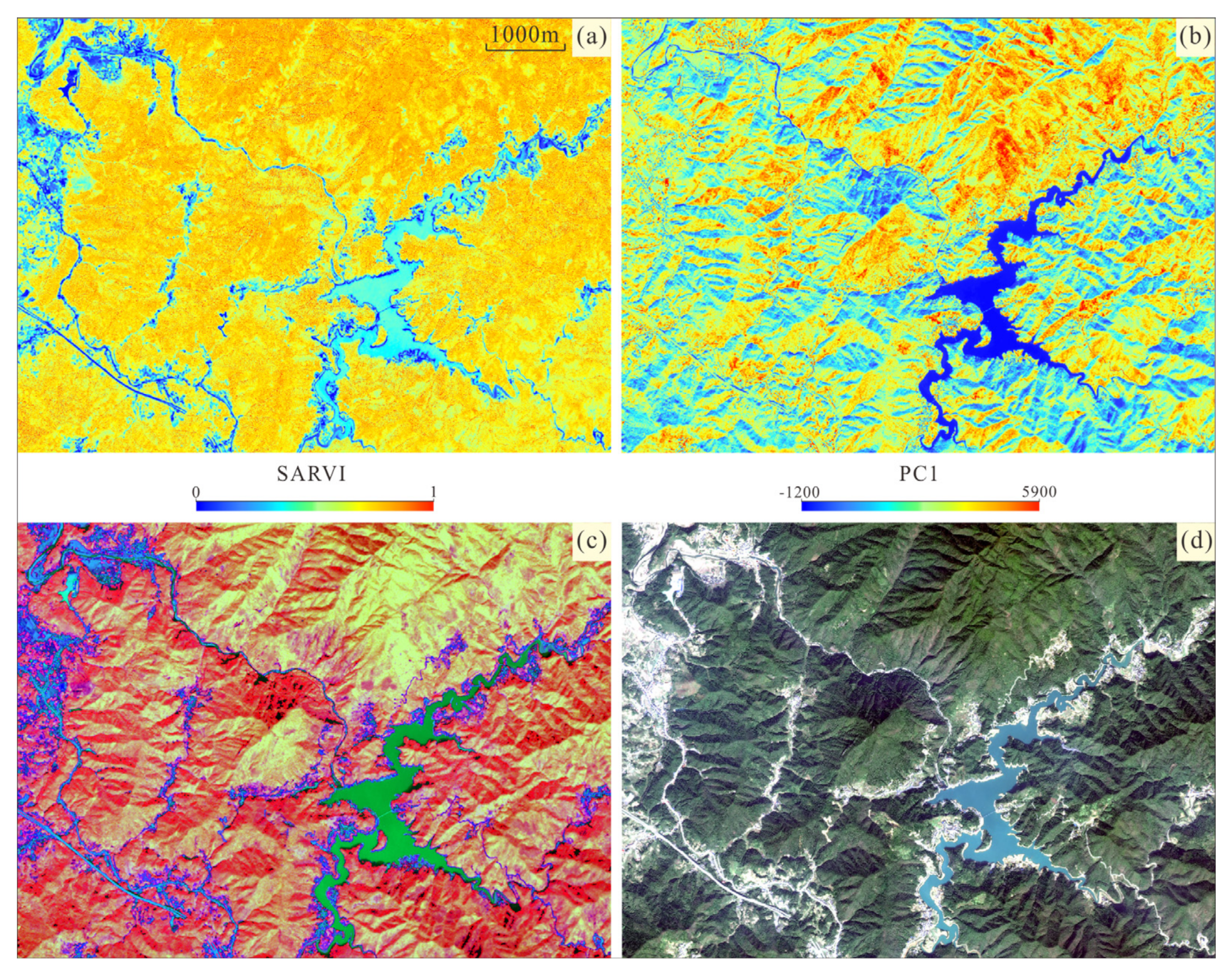
Aiming for precise land classification, four kinds of factors were considered for generating the classification dataset (Figure 6): (1) the SARVI calculated by Equation (1) and the vegetation and no-vegetation areas are distinguished in Figure 6a; (2) the first component (PC-1) of the PCA using bands 1, 2, 3, and 4 includes 87.42% of the eigenvalue (Figure 6b); (3) the HSV space image was generated by Munsell HSV transformation from the pseudo color image (PCI) composed of bands 3 (R), 2 (G), and 1 (B), and it can facilitate identifying soil and rocks as bare lands (Figure 6c); (4) the useless information of the TCI is depressed by convolution filtering, which helps distinguish between the land cover classes in the filtered image (Figure 6d).
The RF-based land cover classification model is constructed with the parameter of 168 trees and three randomly selected features within EnMap-Box [70]. The performance parameters and variable importance can be calculated by applying the constructed model to the validation set. Table 4 shows the obtained confusion matrix based on the classification result and validation set. The number of correctly classified grid cells in each class is displayed in bold on the diagonal matrix. The minimum F1 score calculated from this matrix is 92.28%, pointing to the remarkable performance of the classification model. The high OA of 99.69% and KC of 98.37% suggest that this RF-based model can be successfully used for classification.
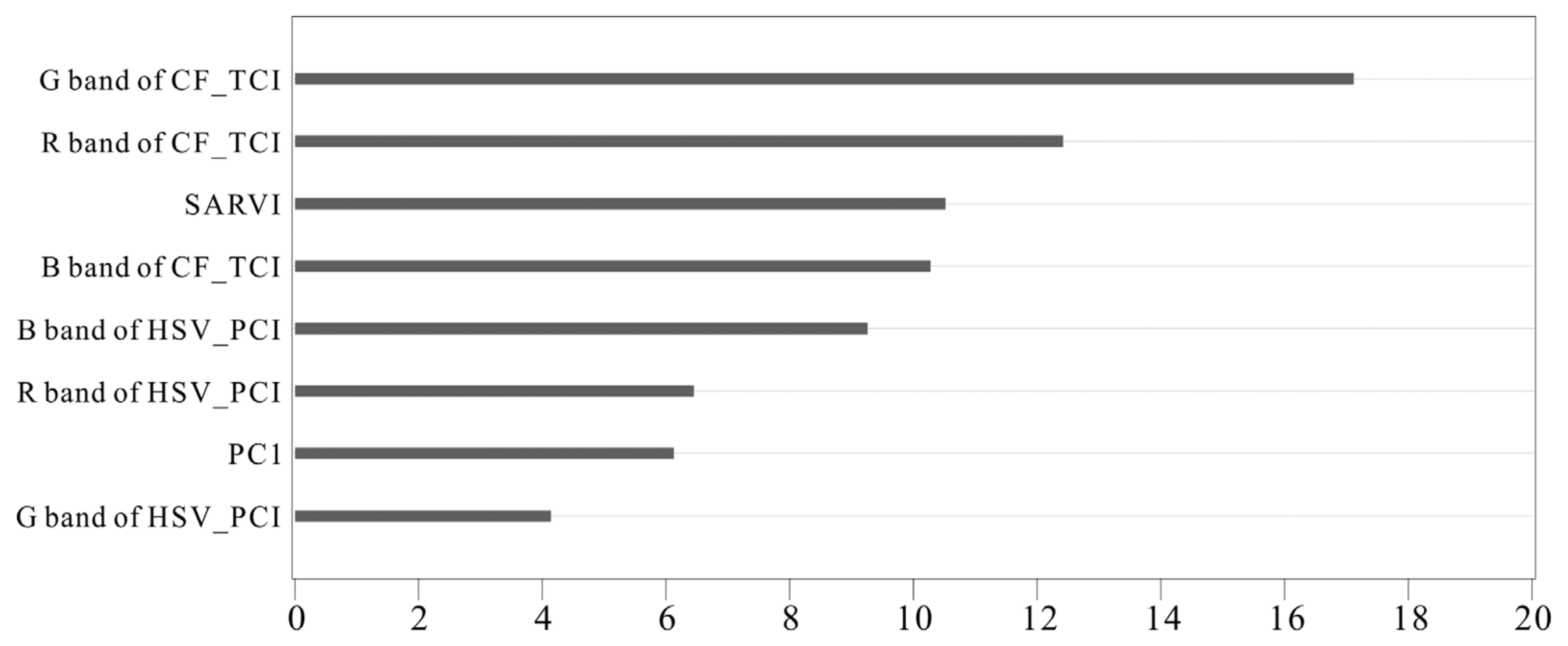
The raw variable importance can indicate its contribution to the generation of every class. It can be seen that the filtering process on the TCI is most favorable for the identification of different land covers, while SARVI comes second, and HSV transformation also performs rather well (Figure 7).
Finally, by applying the RF-based constructed model to the whole dataset, the classification result of the seven-class land cover map is presented in Figure 8. In this study area, the woodland has the highest proportion of up to 81.96%, farmland occupies 8.86%, and the other classes range from 1.19% to 3.42%, except for the tailing area (0.07%). This result is highly consistent with what has been observed in the recent field survey.

4.2. Mining-Induced Geo-Hazard Mapping (MGM)

The actual distribution of the MG occurrences, which is obtained by a large amount of detailed fieldwork, is used as the positive samples, and the places with no MG occurrences are determined as the negative samples. It is important to note that the negative samples should be evenly selected in every land cover class and approximately equal to the positive samples. Here, 24,570 samples, containing 17,126 training samples and 7444 validation samples, are used for training and testing the RF-based prediction model (Figure 9).
Under the guidance of experts and former field investigations, stratigraphic lithology, geological structure, topographical features, road distribution, and rainfall rates are usually used as the predictive factors for MGM. There is no need for information on rainfall because the study area is only about 41 km2, with no variation in rainfall. In addition, environmental factors related to mining activities should be considered as well as the different spectral information of the surface features. Accordingly, the eight predictive factor layers are determined as follows:
(1) Lithology: the lithology layer with twelve types of lithological information is generated from the geological map (Figure 2). Different lithology of the strata possesses different physical structures, resulting in different degrees of weathering and fragmentation.
(2) Land cover map: based on GF-1/PMS data and RF classifier, a land cover map was produced (Section 4.1), and this factor layer is shown in Figure 8.
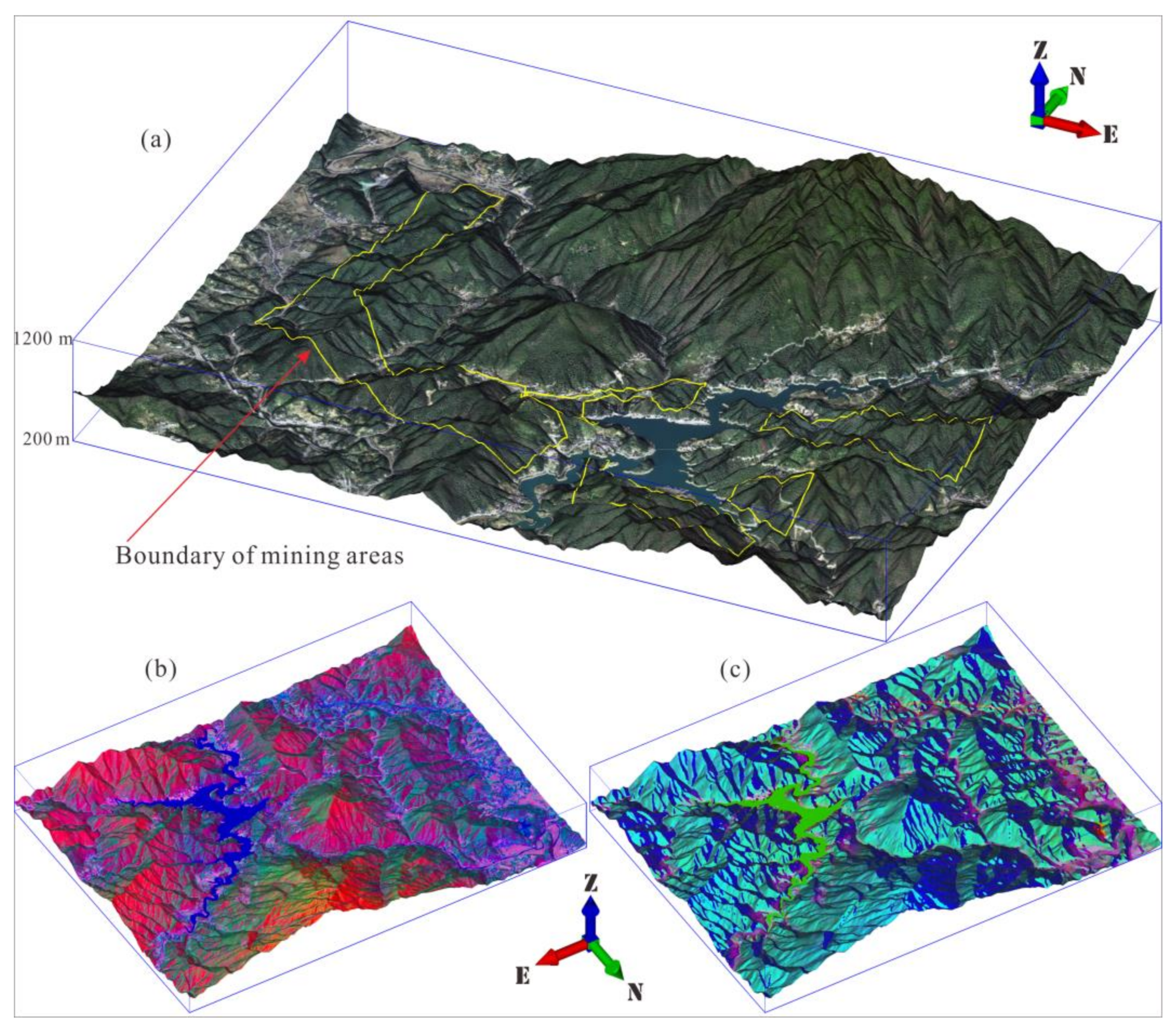
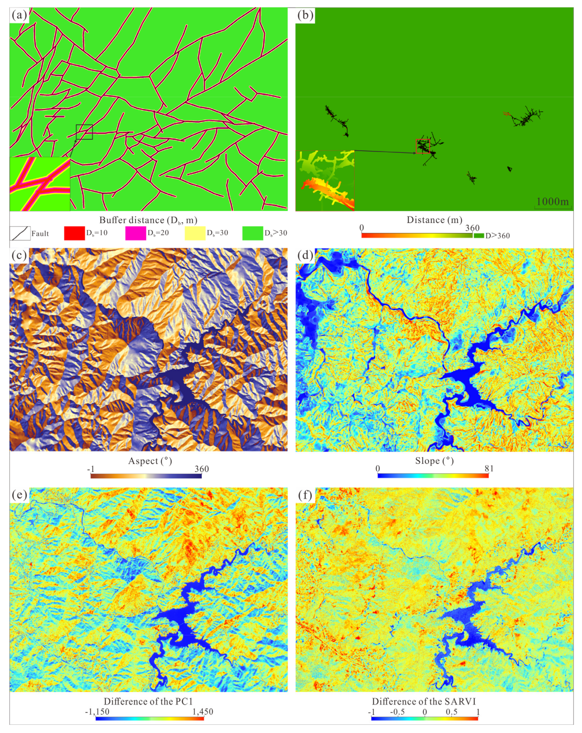
(3) Structure: geological structure, especially the faults, has a strong relationship with MG. As Figure 2 shows, the identified structures are only distributed around mining areas, so the detailed structures of the whole study area need to be reinterpreted. Here, the three-dimension (3D) terrain surface is modeled using triangulated irregular network (TIN) and discrete smooth interpolation (DSI) within GOCAD platform based on a topographic map of 1:2000 on scale. Simultaneously, the noise of the spatial-resolution-improved multispectral bands (1, 2, 3, and 4) are depressed by morphological filtering, and the PC-1 of PCA that is carried out on the filtered result can be used to generate new PCI combining with the other two original bands. Finally, the TCI and two PCIs (enhanced in ENVI) are displayed on a 3D terrain model within MICROMINE (Figure 10). In this way, the faults are easily extracted from these 3D displays through visual interpretation with the help of geologic recognition. The MG occurrences are associated with the distance to faults, and thus, the buffer zones of faults are constructed using three buffer radii of 10, 20, and 30 m, and the distance that is greater than 30 m is set to a value of 999 (Figure 11a) because this distance interval does not affect the MG occurrence under normal circumstances in the study area.
(4) Elevation difference: underground excavation, e.g., tunnels, stopes, and blasting area, will change the stability of strata in the mining areas, and this may lead to surface deformation. The minimum height difference between the surface and the underground mining sites is calculated from the field survey data (Figure 11b).
(5) Aspect and slope: these two property values from topographic features have been proven to be useful for the assessment of MG [27,46,71]. Constructed 3D terrain model can be transformed into a digital elevation model (DEM), and then the aspect and slope of every grid cell can be calculated from the DEM in ArcGIS (Figure 11c,d).
(6) Difference netween the PC-1 and SARVI: as mentioned before, most information of the multispectral bands can be presented in PC-1 using PCA. The SARVI is conducive to distinguish vegetation greenness between different land cover classes, and their difference from different years indicates the changes of the terrain surface. The GF-1/PMS data in the same acquisition phase of 2015 and 2020, in which spatial resolution is improved to 2m with the panchromatic band, are used to calculate SARVI and PC-1, and the difference between these two indexes is shown in Figure 11e,f.
The pixel-based values of every predictive factor layer with the samples layer were extracted as the data vector from their respective raster layers, and then these vectors were combined into a matrix, the dataset for training and prediction consisting of 10,312,500 rows and 9 columns in R. The RF-based prediction model was constructed using positive and negative sample sets (Figure 9) in the data matrix with optimal parameters, i.e., 108 trees and three randomly selected features. Meanwhile, its out-of-bag error (OOB Error) is 1.80%, which indicates a good classification performance. By applying the constructed model to the validation set, 3696 negative samples out of 3796 were correctly classified and 3705 positive samples out of 3722 were correctly predicted. Accordingly, the OA of 98.53% and KC of 97.06% were calculated. In addition, the acquired high AUC value of 0.998 suggests that this constructed model has high performance for MGM in this study.
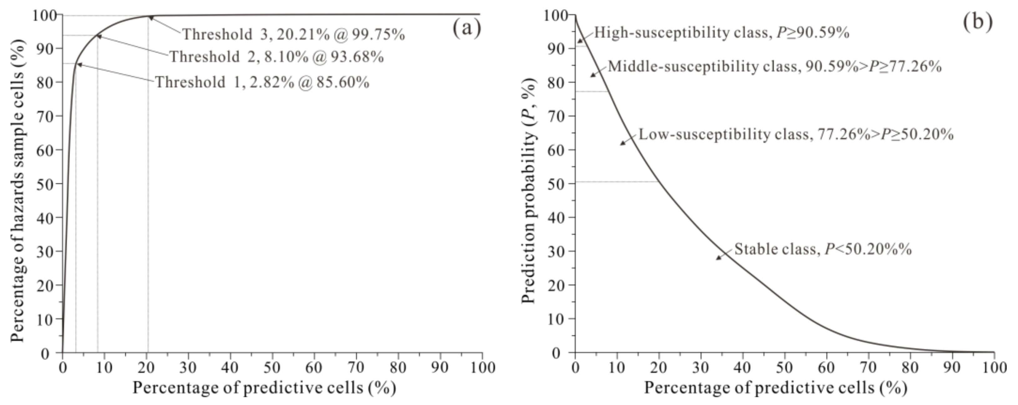
The constructed RF-based prediction model was applied back to the whole data matrix, and every row returned a probability (P) value of classification, containing positive and negative classes. The returned positive class can be considered as the prediction result of MG occurrence probability or susceptibility. The whole dataset is ranked according to the probability values from high to low, and the cumulative percentage of the predictive cells and predicted sample cells can be calculated. Then, the prediction efficiency curve (PEC) and prediction probability curve (PPC) can be plotted (Figure 12). Three thresholds of 1, 2, and 3 were determined on the PEC (Figure 12a), and their corresponding probability values were 90.59%, 77.26%, and 50.20%, respectively (Figure 12b). According to these three thresholds, the whole study area, relative to the occurrence of MG, was divided into four susceptibility classes consisting of high, middle, low, and stable (Figure 13b and Table 5). For the high-susceptibility areas, 2.82% of the total grid cells hold 85.60% of the disaster samples. The stable areas occupy 79.79% of the study area, containing almost no disaster sample.
By qualitatively comparing the terrain surface feature (Figure 10a), land cover map (Figure 8), and MGM (Figure 13), it can be seen that the probability distribution of the MG occurrence is closely related to the places of human activities, such as road excavation, residential area, and mining areas (Figure 13a). In particular, the high susceptibility areas to MG are distributed near the surface excavation and mining areas (Figure 13b).

5. Discussion

5.1. Importance of the Feature Variable

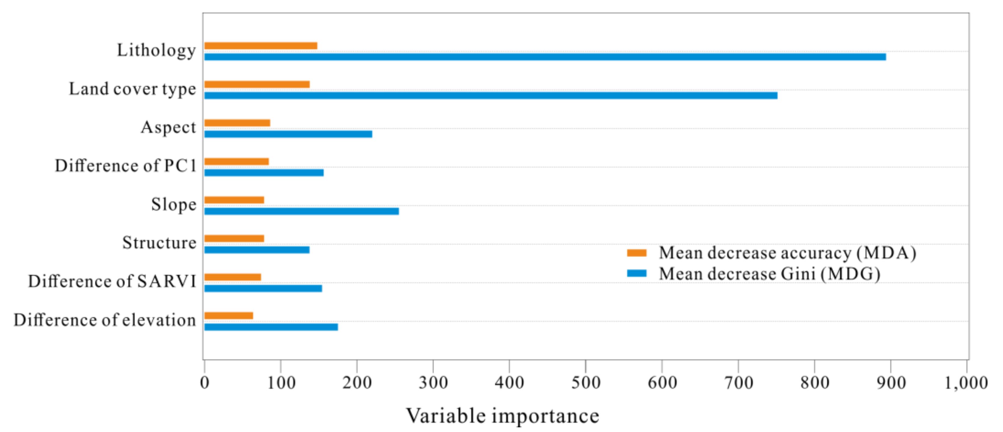
Variable importance is regarded as the contribution to tree node splitting in the generation of the RF-based prediction model, i.e., the contribution of the predictive factors to sample occurrence. The mean decrease accuracy (MDA) and mean decrease Gini (MDG) are two common measures for estimating the variable importance of the RF model. The MDA rankings are more stable than those using MDG, although the higher value of these two indexes indicates the greater contribution of the factor to model construction [72]. Based on the performed importance ranking (Figure 14), we know that the lithology of the strata and the land cover map contributed to the occurrence of the MG more than the other six factors. The faults and underground excavation have been regarded as the critical ones for causing MG, but this result is contrary to our common sense. This highlights the need to quantitatively analyze the correlation of every factor with MG.

5.2. Correlation of the Predictive Factors with MG Occurrence

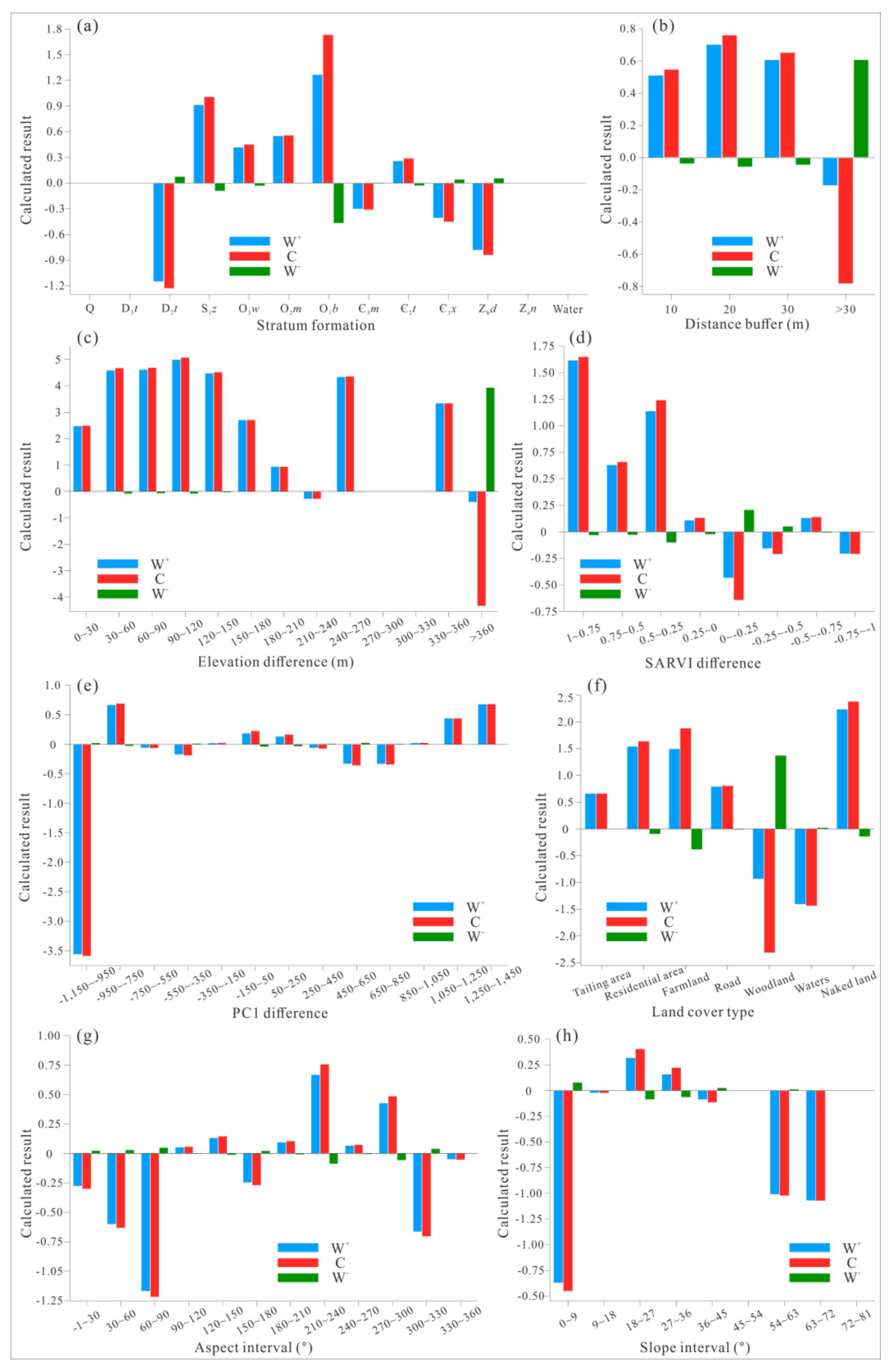
Every predictive factor was divided into different intervals with its property categories (e.g., lithology of the strata, distance buffers of the faults, and the land cover map) or property value (e.g., elevation difference between the terrain surface and the underground excavation, SARVI difference, PC-1 difference, aspect, and slope). Then, the correlation indexes of every interval with MG occurrence, including positive and negative weights (W+ & W) as well as the contrast (C), were calculated by the WofE method and presented in Figure 15.
The factors such as lithology and land cover map that are defined for MGM are closely related to MG occurrence (Figure 15). To be specific, in Figure 15a, the calculated W+ and C values of the Baishuixi Formation are positive and the highest, followed by the Zhoujiaxi, Modao, and Wufeng Formation, illustrating that the stratum holding the shale and sandstone with intercalated carbon-bearing mudstones is the main geological disaster-bearing body. In Figure 15f, for bare land, farmland, residential area, road, and tailing area, their calculated W+ and C values are all positive and greater than those for woodland and waters, showing a clear correlation between human activities and MG occurrence.
In Figure 15b,c, the generated buffers of the faults and the elevation difference between terrain surface and underground tunnels almost obtained greater W+ and C than extremum areas. The buffer distance was more than 30 m, and the elevation difference was more than 360 m, suggesting that these two predictive factors are all in favor of MGM. The SARVI difference in the intervals between 0.25 and 1 showed a close correlation between the decreasing vegetation cover and MG occurrence (Figure 15d). In addition, a higher value of PC-1 difference indicates the increasing probability of the MG occurrence (Figure 15e). Figure 15g,h shows that the MG easily occurred in the surface areas with the features of aspect from 210° to 240° and 270° to 300° and slope from 18° to 36°. Comparative analysis of the results with the later field investigation showed that the aspect and slope of these areas are essentially in agreement with the spatial patterns of the strata outcrop. To sum up, the determination of the eight predictive factors above is reasonable and necessary for MGM.

5.3. MG Monitoring and Pre-Warning

The main purpose of MGM is to monitor and predict the occurrence of future MG, and this work should be continuously focused on the predicted high-susceptibility areas. In addition to monitoring the ground deformation and subsidence using professional GPS equipment and technology, the following precursor information should be captured by visual inspection for MG early-warning: (1) surface and underground excavation, (2) storage or flow changes of water, (3) suddenly bent trees and new fissures or bulges on the ground. Geologically, more attention should be paid to the spatial patterns of stratigraphic formation, especially for places that are highly consistent with the natural or side slope.

6. Conclusions

After more than half a century of mining activities in Liaojiaping Orefield, a series of mining-induced geo-disasters (MG) have been reported. One of the most effective strategies for managing and controlling MG in these mining areas is to identify and map their susceptibility. For this purpose, Gaofen-1 high-resolution satellite images, along with environmental factors identified through geological exploration and topographic survey, were used for mining-induced geo-hazard mapping (MGM) in Liaojiaping Orefield for the first time. RF classifier was used to model the relationship between environmental factors and actual MG events during the MGM, as well as to produce a land cover map. The main findings of this study are summarized as follows:
(1) Using Gaofen-1 high-resolution data, both RF-based binary and multi-class classifiers achieved good performance in land cover mapping and MGM. Some land cover types, e.g., tailing disposal sites, excavated sites, and MG, occupy a small land area. In such cases, a supervised learning algorithm can be used in tandem with high-resolution data to extract samples and detect ground targets.
(2) Based on variable importance analysis, the highest contribution to MGM is related to lithology and land cover among the observed environmental factors, which usually indicate the stability of geological bodies and should be employed to map the geo-disaster susceptibility. In addition, we are able to understand the contribution of variables to the risk modeling through importance analysis of variables; nevertheless, the quantitative analysis of the correlation between the geo-environmental factors and MG based on geostatistical method will allow us to achieve a better understanding of their spatial correlation. In any cases, it is necessary and reasonable to involve all the predictive factors for MGM.
(3) Any changes in land cover, e.g., emerging excavation works and direct vegetation change or degradation, as well as rock bedding creeping in the high susceptibility areas need to be paid high attention to and shall be defined for monitoring and early-warning of MG.

Author Contributions

Y.Q. carried out the fieldwork, conducted the machine learning-based classification and prediction models, analyzed the results, and composed the draft of the paper; L.C. provided the preprocessed Gaofen-1 satellite imagery; A.D.B. revised this manuscript in terms of scientific and English writing; W.W. provided scientific recommendations for this research and revision of the paper. All authors have read and agreed to the published version of the manuscript.

Funding

This work was financially supported by the Start-up Fund for Scientific Research from the East China University of Technology (Grant No. DHBK2019040) and the Open-end Fund from the Key Laboratory of Digital Land and Resources of Jiangxi province (Grant No. DLLJ201901), both granted to Yaozu Qin.

Acknowledgments

The Anhua Xinfeng Mining Co., Ltd. of Hunan Province is acknowledged for providing financial and logistic support to the fieldwork and material collection of this research. Moreover, the constructive comments on this paper by two anonymous reviewers and timely editorial handling by Amiee Shi are highly appreciated.

Conflicts of Interest

We declare that we have no commercial or associative interest that represents a conflict of interest in connection with our work and this manuscript.

References

  1. Marschalko, M.; Yilmaz, I.; Křístková, V.; Fuka, M.; Kubečka, K.; Bouchal, T. An indicative method for determination of the most hazardous changes in slopes of the subsidence basins in underground coal mining area in Ostrava (Czech Republic). Environ. Monit. Assess. 2013, 185, 509–522. [Google Scholar] [CrossRef]
  2. Yang, Y.Y.; Xu, Y.S.; Shen, S.L.; Yuan, Y.; Yin, Z.Y. Mining-induced geo-hazards with environmental protection measures in Yunnan, China: An overview. Bull. Eng. Geol. Environ. 2015, 74, 141–150. [Google Scholar] [CrossRef]
  3. Li, S.L. Study on the geological hazard in metal mines and its prevention countermeasures. Chin. J. Geol. Hazard Control 2002, 46–50+54, (In Chinese with English Abstract). [Google Scholar]
  4. Yi, H.P.; Jiang, Z. Causes and prevention measures of mine geological disasters. Sci. Technol. Innov. Her. 2010, 4, 126. (In Chinese) [Google Scholar]
  5. Fan, L.M.; Li, C.; Chen, J.P.; Ning, J.M. Geological hazards and prevention technology in high-intensity mining area of mineral resources. Sci. Press 2016, 28, 8. (In Chinese) [Google Scholar]
  6. Liu, L.; Chen, L.Q.; Tang, J.X. Present Situation and Future Prospects of Geologic Environment Issues in Mines in China. Disaster Adv. 2010, 3, 563–566. [Google Scholar]
  7. Shao, L.F. Geological disaster prevention and control and resource protection in mineral resource exploitation region. Int. J. Low-Carbon Technol. 2019, 14, 142. [Google Scholar] [CrossRef] [Green Version]
  8. Xu, Y.N. Investigation and research on the mine geological environment: Present status and outlook. Geol. Bull. China 2008, 27, 1235–1244, (In Chinese with English Abstract). [Google Scholar]
  9. Chowdhury, R.; Flentje, P. Role of slope reliability analysis in landslide risk management. Bull. Eng. Geol. Environ. 2003, 62, 41–46. [Google Scholar] [CrossRef]
  10. Romeo, R.W.; Floris, M.; Veneri, F. Area-scale landslide hazard and risk assessment. Environ. Geol. 2006, 51, 1–13. [Google Scholar] [CrossRef]
  11. Huang, R.Q.; Li, W.L. Analysis of the geo-hazards triggered by the 12 May 2008 Wenchuan earthquake, China. Bull. Eng. Geol. Environ. 2009, 68, 363–371. [Google Scholar] [CrossRef]
  12. Chen, K.T.; Wu, J.H. Simulating the failure process of the xinmo landslide using discontinuous deformation analysis. Eng. Geol. 2018, 239, 269–281. [Google Scholar] [CrossRef]
  13. Wang, Q.J.; Guo, H.D.; Chen, Y.; Lin, Q.Z.; Li, H. Application of remote sensing for investigating mining geological hazards. Int. J. Digit. Earth 2013, 6, 449–468. [Google Scholar] [CrossRef]
  14. Segoni, S.; Pappafico, G.; Luti, T.; Catani, F. Landslide susceptibility assessment in complex geological settings: Sensitivity to geological information and insights on its parameterization. Landslides 2020, 17, 2443–2453. [Google Scholar] [CrossRef] [Green Version]
  15. Ahmad, H.; Chen, N.S.; Rahman, M.; Islam, M.M.; Pourghasemi, H.R.; Habumugisha, J.M. Geohazards Susceptibility Assessment along the Upper Indus Basin Using Four Machine Learning and Statistical Models. ISPRS Int. J. Geo-Inf. 2021, 10, 315. [Google Scholar] [CrossRef]
  16. Westen, C.J.V.; Castellanos, E.; Kuriakose, S.L. Spatial data for landslide susceptibility, hazard, and vulnerability assessment: An overview. Eng. Geol. 2008, 102, 112–131. [Google Scholar] [CrossRef]
  17. Lu, P.; Catani, F.; Tofani, V.; Casagli, N. Quantitative hazard and risk assessment for slow-moving landslides from persistent scatterer interferometry. Landslides 2014, 11, 685–696. [Google Scholar] [CrossRef]
  18. Pavlova, I.; Makarigakis, A.; Depret, T.; Jomelli, V. Global overview of the geological hazard exposure and disaster risk awareness at world heritage sites. J. Cult. Herit. 2017, 28, 8445–8452. [Google Scholar] [CrossRef]
  19. Vaziri, V.; Hamidi, J.K.; Sayadi, A.R. An integrated GIS-based approach for geohazards risk assessment in coal mines. Environ. Earth Sci. 2018, 77, 29. [Google Scholar] [CrossRef]
  20. Mohammady, M.; Pourghasemi, H.R.; Amiri, M. Assessment of land subsidence susceptibility in Semnan plain (Iran): A comparison of support vector machine and weights of evidence data mining algorithms. Nat. Hazards 2019, 99, 951–971. [Google Scholar] [CrossRef]
  21. Hemasinghe, H.; Rangali, R.S.; Deshapriya, N.L.; Samarakoon, L. Landslide susceptibility mapping using logistic regression model (a case study in Badulla District, Sri Lanka). Procedia Eng. 2018, 212, 1046–1053. [Google Scholar] [CrossRef]
  22. Lee, H.; Oh, J. Establishing an ANN-Based Risk Model for Ground Subsidence Along Railways. Appl. Sci. 2018, 8, 1936. [Google Scholar] [CrossRef] [Green Version]
  23. Youssef, A.M.; Pourghasemi, H.R.; Pourtaghi, Z.S.; Al-Katheeri, M.M. Landslide susceptibility mapping using random forest, boosted regression tree, classification and regression tree, and general linear models and comparison of their performance at Wadi Tayyah Basin, Asir Region, Saudi Arabia. Landslides 2016, 13, 839–856. [Google Scholar] [CrossRef]
  24. Zhang, K.X.; Wu, X.L.; Niu, R.Q.; Yang, K.; Zhao, L.R. The assessment of landslide susceptibility mapping using random forest and decision tree methods in the Three Gorges Reservoir area, China. Environ. Earth Sci. 2017, 76, 405. [Google Scholar] [CrossRef]
  25. Kim, K.D.; Lee, S.; Oh, H.J.; Choi, J.K.; Won, J.S. Assessment of ground subsidence hazard near an abandoned underground coal mine using GIS. Environ. Geol. 2006, 50, 1183–1191. [Google Scholar] [CrossRef]
  26. Sharma, S.; Mahajan, A.K. A comparative assessment of information value, frequency ratio and analytical hierarchy process models for landslide susceptibility mapping of a Himalayan watershed, India. Bull. Eng. Geol. Environ. 2019, 78, 2431–2448. [Google Scholar] [CrossRef]
  27. Zhou, X.T.; Wu, W.C.; Lin, Z.Y.; Zhang, G.L.; Chen, R.X.; Song, Y.; Wang, Z.L.; Lang, T.; Qin, Y.Z.; Ou, P.H.; et al. Zonation of Landslide Susceptibility in Ruijin, Jiangxi, China. Int. J. Environ. Res. Public Health 2021, 18, 5906. [Google Scholar] [CrossRef] [PubMed]
  28. Cracknell, M.J.; Reading, A.M. Geological mapping using remote sensing data: A comparison of five machine learning algorithms, their response to variations in the spatial distribution of training data and the use of explicit spatial information. Comput. Geosci. 2014, 63, 22–33. [Google Scholar] [CrossRef] [Green Version]
  29. Carranza, E.J.M.; Laborte, A.G. Random Forest predictive modeling of mineral prospectivity with small number of prospects and data with missing values in Abra (Philippines). Comput. Geosci. 2015, 74, 60–70. [Google Scholar] [CrossRef]
  30. Li, X.H. Using “random forest” for classification and regression. Chin. J. Appl. Entomol. 2016, 50, 1190–1197. [Google Scholar]
  31. Qin, Y.Z.; Liu, L.M. Quantitative 3D Association of Geological Factors and Geophysical Fields with Mineralization and Its Significance for Ore Prediction: An Example from Anqing Orefield, China. Minerals 2018, 8, 300. [Google Scholar] [CrossRef] [Green Version]
  32. Wu, W.C.; Zucca, C.; Muhaimeed, A.S.; Alshafie, W.M.; Alquraish, A.M.F.; Nangia, V.; Zhu, M.Q.; Liu, G.P. Soil salinity prediction and mapping by machine learning regression in Central Mesopotamia. Land Degrad. Dev. 2018, 29, 4005–4014. [Google Scholar] [CrossRef]
  33. Sun, T.; Li, H.; Wu, K.; Chen, F.; Zhu, Z.; Hu, Z. Data-Driven Predictive Modelling of Mineral Prospectivity Using Machine Learning and Deep Learning Methods: A Case Study from Southern Jiangxi Province, China. Minerals 2020, 10, 102. [Google Scholar] [CrossRef] [Green Version]
  34. Cao, J.; Zhang, Z.; Du, J.; Zhang, L.; Song, Y.; Sun, G. Multi-geohazards susceptibility mapping based on machine learning—A case study in Jiuzhaigou, China. Nat. Hazards 2020, 102, 851–871. [Google Scholar] [CrossRef]
  35. Magidi, J.; Nhamo, L.; Mpandeli, S.; Mabhaudhi, T. Application of the Random Forest Classifier to Map Irrigated Areas Using Google Earth Engine. Remote Sens. 2021, 13, 876. [Google Scholar] [CrossRef]
  36. Choi, W.; Lee, H.; Kim, D.; Kim, S. Improving Spatial Coverage of Satellite Aerosol Classification Using a Random Forest Model. Remote Sens. 2021, 13, 1268. [Google Scholar] [CrossRef]
  37. Qin, Y.Z.; Liu, L.M.; Wu, W.C. Machine Learning-Based 3D Modeling of Mineral Prospectivity Mapping in the Anqing Orefield, Eastern China. Nat. Resour. Res. 2021. [Google Scholar] [CrossRef]
  38. Youssef, A.M.; Pourghasemi, H.R. Landslide susceptibility mapping using machine learning algorithms and comparison of their performance at Abha Basin, Asir Region, Saudi Arabia. Geosci. Front. 2021, 12, 639–655. [Google Scholar] [CrossRef]
  39. Shao, L.; Li, J. Geological hazards types induced by mining and their characteristics in Guizhou province. Chin. J. Geol. Hazards Control. 2011, 22, 56–60, (In Chinese with English Abstract). [Google Scholar]
  40. Kong, F.J.; Li, X.B.; Hong, W.; Xie, D.F.; Li, X.; Bai, Y.X. Land cover classification based on fused data from gf-1 and modis ndvi time series. Remote Sens. 2016, 8, 741. [Google Scholar] [CrossRef] [Green Version]
  41. Yang, C.; Wu, G.F.; Kai, D.; Shi, T.Z.; Li, Q.Q.; Wang, J.L. Improving land use/land cover classification by integrating pixel unmixing and decision tree methods. Remote Sens. 2017, 9, 1222. [Google Scholar] [CrossRef] [Green Version]
  42. Akbari, E.; Boloorani, A.D.; Samany, N.N.; Hamzeh, S.; Soufizadeh, S.; Pignatti, S. Crop Mapping Using Random Forest and Particle Swarm Optimization based on Multi-Temporal Sentinel-2. Remote Sens. 2020, 12, 1449. [Google Scholar] [CrossRef]
  43. Youssef, A.M. Landslide susceptibility delineation in the Ar-Rayth area, Jizan, Kingdom of Saudi Arabia, using analytical hierarchy process, frequency ratio, and logistic regression models. Environ. Earth Sci. 2015, 73, 8499–8518. [Google Scholar] [CrossRef]
  44. Pachuau, L. Zonation of Landslide Susceptibility and Risk Assessment in Serchhip town, Mizoram. J. Indian Soc. Remote Sens. 2019, 47, 1587–1597. [Google Scholar] [CrossRef]
  45. Arabameri, A.; Pradhan, B.; Rezaei, K.; Lee, C.W. Assessment of Landslide Susceptibility Using Statistical- and Artificial Intelligence-Based FR-RF Integrated Model and Multiresolution DEMs. Remote Sens. 2019, 11, 999. [Google Scholar] [CrossRef] [Green Version]
  46. Zhang, Y.; Wu, W.C.; Qin, Y.Z.; Lin, Z.Y.; Zhang, G.L.; Chen, R.X.; Song, Y.; Lang, T.; Zhou, X.T.; Huangfu, W.C.; et al. Mapping Landslide Hazard Risk Using Random Forest Algorithm in Guixi, Jiangxi, China. Int. J. Geo-Inf. 2020, 9, 695. [Google Scholar] [CrossRef]
  47. Ou, P.H.; Wu, W.C.; Qin, Y.Z.; Zhou, X.T.; Huangfu, W.C.; Zhang, Y.; Xie, L.F.; Fu, X.; Li, J.; Jiang, J.H.; et al. Assessment of landslide hazard in jiangxi using geo-information. Front. Earth Sci. China 2021, 9, 648342. [Google Scholar] [CrossRef]
  48. Micheletti, N.; Foresti, L.; Robert, S.; Leuenberger, M.; Pedrazzini, A.; Jaboyedoff, M.; Kanevski, M. Machine Learning Feature Selection Methods for Landslide Susceptibility Mapping. Math. Geosci. 2014, 46, 33–57. [Google Scholar] [CrossRef] [Green Version]
  49. Bai, Z.G. Technical characteristics of the Gaofen-1 Satellite. Aerosp. China 2013, 8, 5–9. (In Chinese) [Google Scholar]
  50. Gao, H.L.; Gu, X.F.; Yu, T.; Sun, Y.; Xie, Y.; Liu, Q.Y. Validation of the calibration coefficient of the gaofen-1 pms sensor using the landsat 8 oli. Remote. Sens. 2016, 8, 132. [Google Scholar] [CrossRef] [Green Version]
  51. Goetz, J.N.; Brenning, A.; Petschko, H.; Leopold, P. Evaluating machine learning and statistical prediction techniques for landslide susceptibility modeling. Comput. Geosci. 2015, 81, 1–11. [Google Scholar] [CrossRef]
  52. Moosavi, V.; Niazi, Y. Development of hybrid wavelet packet-statistical models (WP-SM) for landslide susceptibility mapping. Landslides 2016, 13, 97–114. [Google Scholar] [CrossRef]
  53. Dou, J.; Yunus, A.P.; Bui, D.T.; Merghadi, A.; Sahana, M.; Zhu, Z.F.; Chen, C.W.; Khosravi, K.; Yang, Y.; Pham, B.T. Assessment of advanced random forest and decision tree algorithms for modeling rainfall-induced landslide susceptibility in the Izu-Oshima Volcanic Island, Japan. Sci. Total Environ. 2019, 662, 332–346. [Google Scholar] [CrossRef]
  54. Kalantar, B.; Pradhan, B.; Naghibi, S.A.; Motevalli, A.; Mansor, S. Assessment of the effects of training data selection on the landslide susceptibility mapping: A comparison between support vector machine (SVM), logistic regression (LR) and artificial neural networks (ANN). Geomat. Nat. Hazards Risk 2018, 9, 49–69. [Google Scholar] [CrossRef]
  55. Schowengerdt, R.A. Remote Sensing: Models & Methods for Image Processing, 3rd ed.; Academic Press: Orlando, FL, USA, 2006. [Google Scholar]
  56. Kaufman, Y.J.; Tanre, D. Atmospherically resistant vegetation index (ARVI) for eos-modis. IEEE Trans. Geosci. Remote. Sens. 1992, 30, 261–270. [Google Scholar] [CrossRef]
  57. Huete, A.R. A soil-adjusted vegetation index (SAVI). Remote Sens. Environ. 1988, 25, 295–309. [Google Scholar] [CrossRef]
  58. Escadafal, R.; Girard, M.C.; Courault, D. Munsell soil color and soil reflectance in the visible spectral bands of landsat mss and tm data. Remote Sens. Environ. 1989, 27, 37–46. [Google Scholar] [CrossRef]
  59. Hotelling, H. Analysis of a Complex of Statistical Variables into Principal Components. J. Educ. Psychol. 1933, 24, 417–441, 498–520. [Google Scholar] [CrossRef]
  60. Cichocki, A.; Amari, S. Adaptive Blind Signal and Image Processing: Learning Algorithms and Applications; Wiley: New York, NY, USA, 2002; p. 586. [Google Scholar]
  61. Breiman, L. Random forests. Mach. Learn. 2001, 45, 5–32. [Google Scholar] [CrossRef] [Green Version]
  62. Quinlan, J.R. Induction of Decision Trees. Mach. Learn. 1996, 1, 81–106. [Google Scholar] [CrossRef] [Green Version]
  63. Breiman, L.; Friedman, J.H.; Olshen, R.A.; Stone, C.J. Classification and regression trees (cart). Biometrics 1984, 40, 358. [Google Scholar]
  64. Breiman, L. Bagging predictors. Mach. Learn. 1996, 24, 123–140. [Google Scholar] [CrossRef] [Green Version]
  65. Ho, T.K. The random subspace method for constructing decision forests. IEEE Trans. Pattern Anal. Mach. Intell. 1998, 20, 832–844. [Google Scholar]
  66. Lee, D.H.; Kim, Y.T.; Lee, S.R. Shallow Landslide Susceptibility Models Based on Artificial Neural Networks Considering the Factor Selection Method and Various Non-Linear Activation Functions. Remote Sens. 2020, 12, 1194. [Google Scholar] [CrossRef] [Green Version]
  67. Agterberg, F.P. Systematic approach to dealing with uncertainty of geoscience information in mineral exploration. In Proceedings of the 21st APCOM Symposium, Las Vegas, NV, USA, March 1989; Chapter 18. pp. 165–178. [Google Scholar]
  68. Bonham-Carter, G.F.; Agterberg, F.P.; Wright, D.F. Weights of evidence modeling: A new approach to mapping mineral potential. Geol. Surv. Can. 1989, 89, 171–183. [Google Scholar]
  69. Agterberg, F.P.; Bonham-Carter, G.F.; Cheng, Q.; Wright, D.F. Weights of evidence modeling and weighted logistic regression for mineral potential mapping. In Computers in Geology—25 Years of Progress; Oxford University Press, Inc.: Oxford, UK, 1993; pp. 13–32. [Google Scholar]
  70. Waske, B.; van der Linden, S.; Oldenburg, C.; Jakimow, B.; Rabe, A.; Hostert, P. imageRF—A user-oriented implementation for remote sensing image analysis with random forests. Environ. Modeling Softw. 2012, 35, 192–193. [Google Scholar] [CrossRef]
  71. Pradhan, B.; Lee, S. Landslide susceptibility assessment and factor effect analysis: Backpropagation artificial neural networks and their comparison with frequency ratio and bivariate logistic regression modelling. Environ. Model. Softw. 2010, 25, 747–759. [Google Scholar] [CrossRef]
  72. Nicodemus, K.K. Letter to the Editor: On the stability and ranking of predictors from random forest variable importance measures. Brief. Bioinform. 2011. [Google Scholar] [CrossRef] [Green Version]
Figure 1. Location of the Hunan province in China (a), the study area in Hunan province (b) and the geological settings of the Liaojiaping Orefield (c).
Remotesensing 13 03638 g001
Figure 2. Geological map of the Liaojiaping Orefield, showing the main stratigraphic units, faults, water body, and the main mining areas, including (a) Taiping–Tanchelun, (b) Babaoshan, (c) Xiaojiawan, (d) Niejialing, and (e) Tianshenghe.
Remotesensing 13 03638 g002
Figure 3. Mining-induced geo-disasters (MG) in the Liaojiaping Orefield, showing the different types and scales, (a,b): landslide, (c,d): subsidence, (e): collapse, and (f): ground fissure.
Remotesensing 13 03638 g003
Figure 4. Improving the process of GM sample occurrence, (a) show the occurrence areas (vector), (b) are their grid form (raster), and (c) are the training points converted from samples.
Remotesensing 13 03638 g004
Figure 5. Ground truth datasets for land cover mapping: (a) training set and (b) validation set.
Remotesensing 13 03638 g005
Figure 6. Determined classification factors for land cover mapping: (a) SARVI, (b) PC-1, (c) HSV_PCI, RGB color image from HSV space transformation (bands 4, 3, and 1), and (d) CF_TCI, RGB color image from convolution filtering (bands 3, 2, and 1).
Remotesensing 13 03638 g006
Figure 7. Contribution ranking of each classification factor to the RF-based classifier.
Remotesensing 13 03638 g007
Figure 8. The obtained RF-based 2 m resolution land cover map of the study area using GF-1/PMS imagery.
Remotesensing 13 03638 g008
Figure 9. Spatial distribution of the acquired positive and negative samples in the training and validation sets for construction of RF-based prediction model for MGM of the study area.
Remotesensing 13 03638 g009
Figure 10. The 3D visualization of the terrain surface, showing the TCI (a) and two enhanced PCI (b,c) from GF-1/PMS imagery.
Remotesensing 13 03638 g010
Figure 11. Predictive factor layers: (a) distance buffers of the structure, (b) difference in elevation between underground excavation and surface, (c,d) aspect and slope, and (e,f) difference between the PC-1 and SARVI.
Remotesensing 13 03638 g011
Figure 12. Analysis of capture-efficiency curve (a,b) prediction probability curve for zonation of the MGM.
Remotesensing 13 03638 g012
Figure 13. The 3D display of the MGM, showing (a) the probability distribution and (b) zonation of the MG susceptibility areas.
Remotesensing 13 03638 g013
Figure 14. Ranking of predictive factors’ contribution to RF-based prediction modeling.
Remotesensing 13 03638 g014
Figure 15. Calculated results of WofE, showing the different predictive factors: (a) lithology of the strata, (b) distance buffers of the faults, (c) elevation difference between the underground excavations and the surface, (d) SARVI difference, (e) PC-1 difference, (f) land cover, (g) aspect, and (h) slope.
Remotesensing 13 03638 g015
Table 1. Detailed stratigraphy of the Liaojiaping Orefield.
EpochLithological UnitCodeThickness and Lithological Composition
QuaternaryNoQ1~3 m. Eluvium and alluvium: thin clay and clayey soil.
Upper DevonianTianxin FormationD3t180~400 m. Thin-bedded siltstone, silty shale.
Middle DevonianTiaomajian FormationD2tMore than 660 m. Silty shale with siltstone interblended, thick fine-grained quartzose sandstone intercalated with siltstone and celadon shale.
Lower SilurianZhoujiaxi FormationS1z64~375 m. Medium-thick fine sandstone intercalated with thin layered silty shale, carbonaceous fine sandstone with interlayers of the siltstone.
Upper OrdovicianWufeng FormationO3w5~28 m. Medium-bedded silty carbonaceous platy shale with intercalated siliceous bands.
Middle OrdovicianModao FormationO2m48~80 m. Carbon-bearing silicate with thin silty shale interblended.
Lower OrdovicianBaishuixi FormationO1b150~520 m. Gray plate shale locally intercalated with carbon-bearing mudstone and siliceous bands.
Upper CambrianMiliangpo FormationЄ3m140~320 m. Crystal powder limestone intercalated with siliceous bands.
Middle CambrianTanxi FormationЄ2t110-280 m. Gray banded marlstone and globular crystal powder limestone.
Lower CambrianXiaoyanxi FormationЄ1x158~368 m. Carbonaceous mudstone intercalated with poor coal seam and siliceous bands.
Upper SinianDoushantuo FormationZbd70~121 m. Thin-bedded carbon-bearing mudstone, biomicrite, and silicate layered clearly.
Lower SinianNantuo FormationZan100~680 m. Moraine conglomerate, conglomerate, and carbonate with the character of glaciomarine deposit.
Table 2. Imagery parameters of the GF-1/PMS [50].
SensorSpectral BandWavelength Range (µm)Spatial Resolution (m)
PMSPanchromaticB–1 (PAN)0.45–0.902
MultispectralB–2 (Blue)0.45–0.528
B–3 (Green)0.52–0.59
B–4 (Red)0.63–0.69
B–5 (NIR)0.77–0.89
Table 3. Ground truth sample composition for land cover mapping.
ClassificationNo. of Samples forSample Proportion
TrainingValidationIn Sample SetIn Study Area
Tailing area12585450.1830.017
Residential area325214120.4720.045
Farmland22,90496183.2930.315
Road271811640.3930.038
Woodland621,245266,57889.9028.609
Water body35,80115,3465.1790.496
Bare land410815940.5770.055
Table 4. Accuracy assessment of RF-based land cover classification model.
ClassConfusion Matrix (No. of grid cells)F1 Score
(%)
Class1Class2Class3Class4Class5Class6Class7Sum
Tailing area536 *10200654598.80
Residential area013331140460141295.01
Farmland07935651380112961896.33
Road13011310029116497.16
Woodland0224390266,11016266,57899.89
Waters0700015,339015,34699.96
Naked land3211012001548159492.28
Sum540139498061164266,24815,3441761296,257-
* Diagonal number highlighted in bold indicates the correctly classified cells.
Table 5. Zonation of the MGM.
Susceptibility ClassProbability Interval (P, %)Proportion of the Predictive Data (%)Proportion of the Samples (%)Occurrence Rate of the Samples (%)
HighP ≥ 90.59%2.8285.607.23
Middle90.59% > P ≥ 77.26%5.288.080.36
Low77.26% > P ≥ 50.20%12.116.070.12
StableP < 50.20%79.790.250
Publisher’s Note: MDPI stays neutral with regard to jurisdictional claims in published maps and institutional affiliations.