
A National-Scale 1-km Resolution PM2.5 Estimation Model over Japan Using MAIAC AOD and a Two-Stage Random Forest Model


Abstract
:1. Introduction
2. Materials and Methods
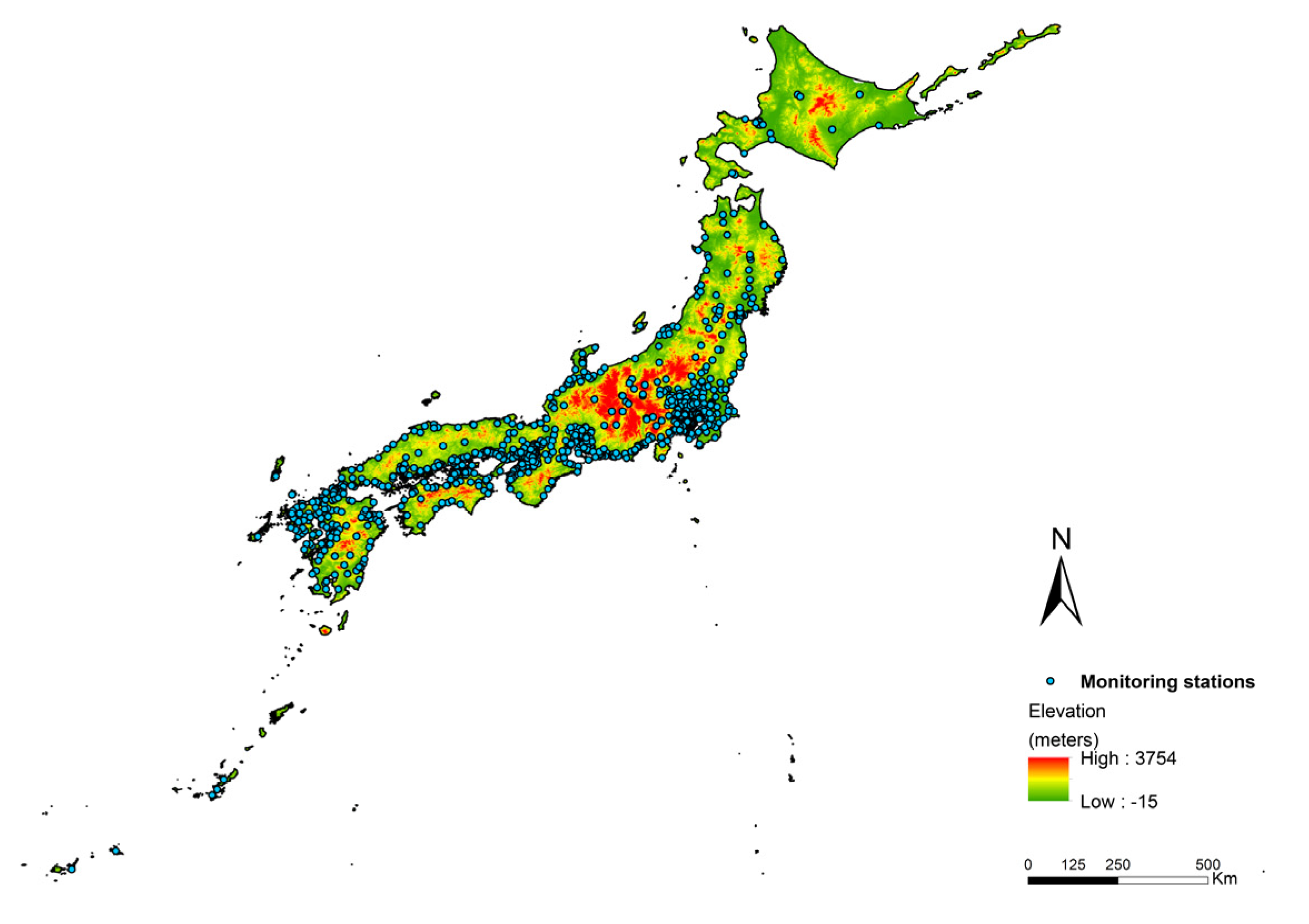
2.1. Study Area
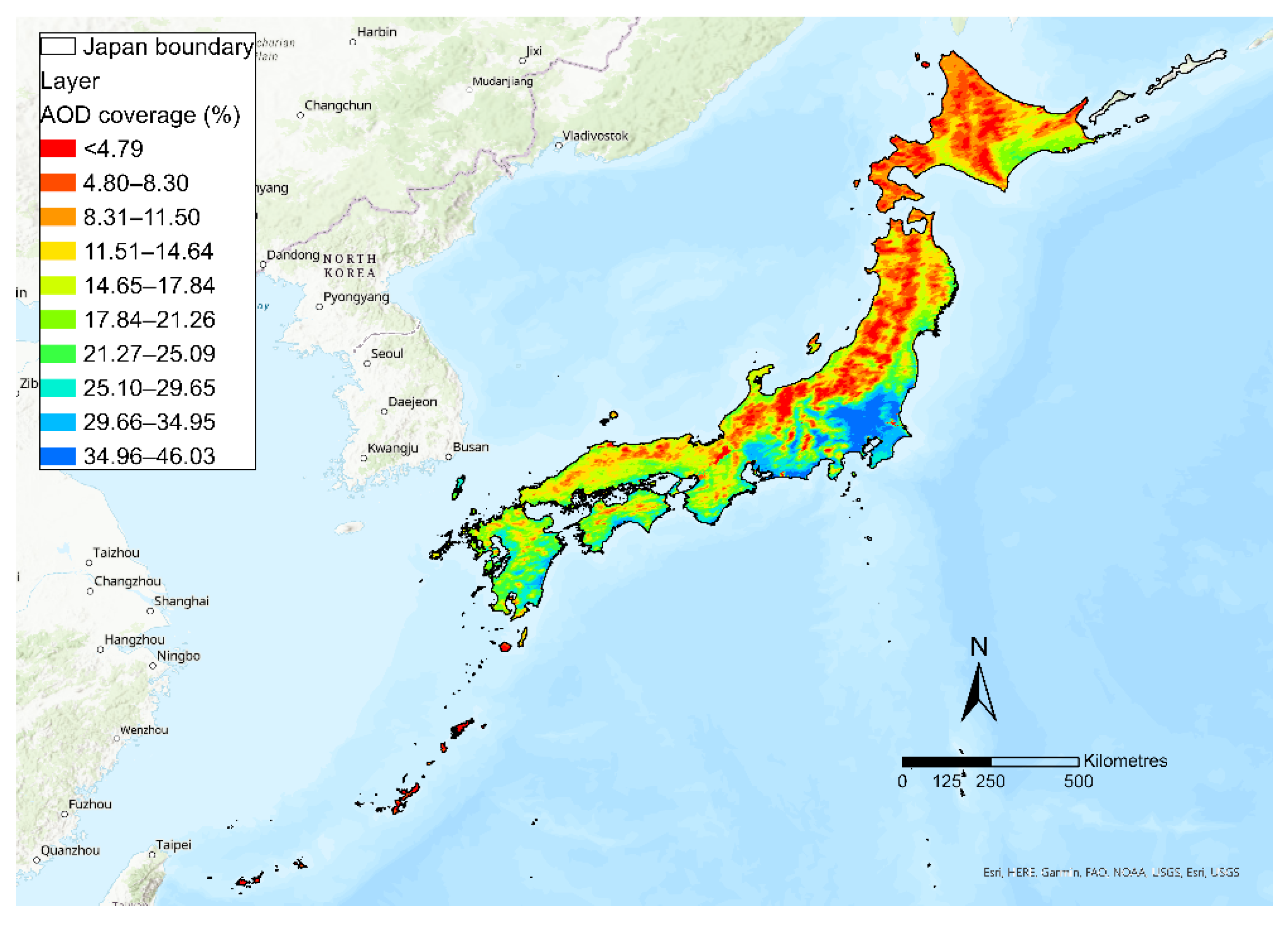
2.2. MAIAC AOD
2.3. AERONET AOD
2.4. Ground PM Measurements
2.5. Meteorological Variables
2.6. Land Use Data
2.7. Population Counts
2.8. Elevation
2.9. Statistical Methods
3. Results
3.1. Validation of MAIAC AOD with Ground Measurements over Japan
3.2. Ground PM2.5 Measurements
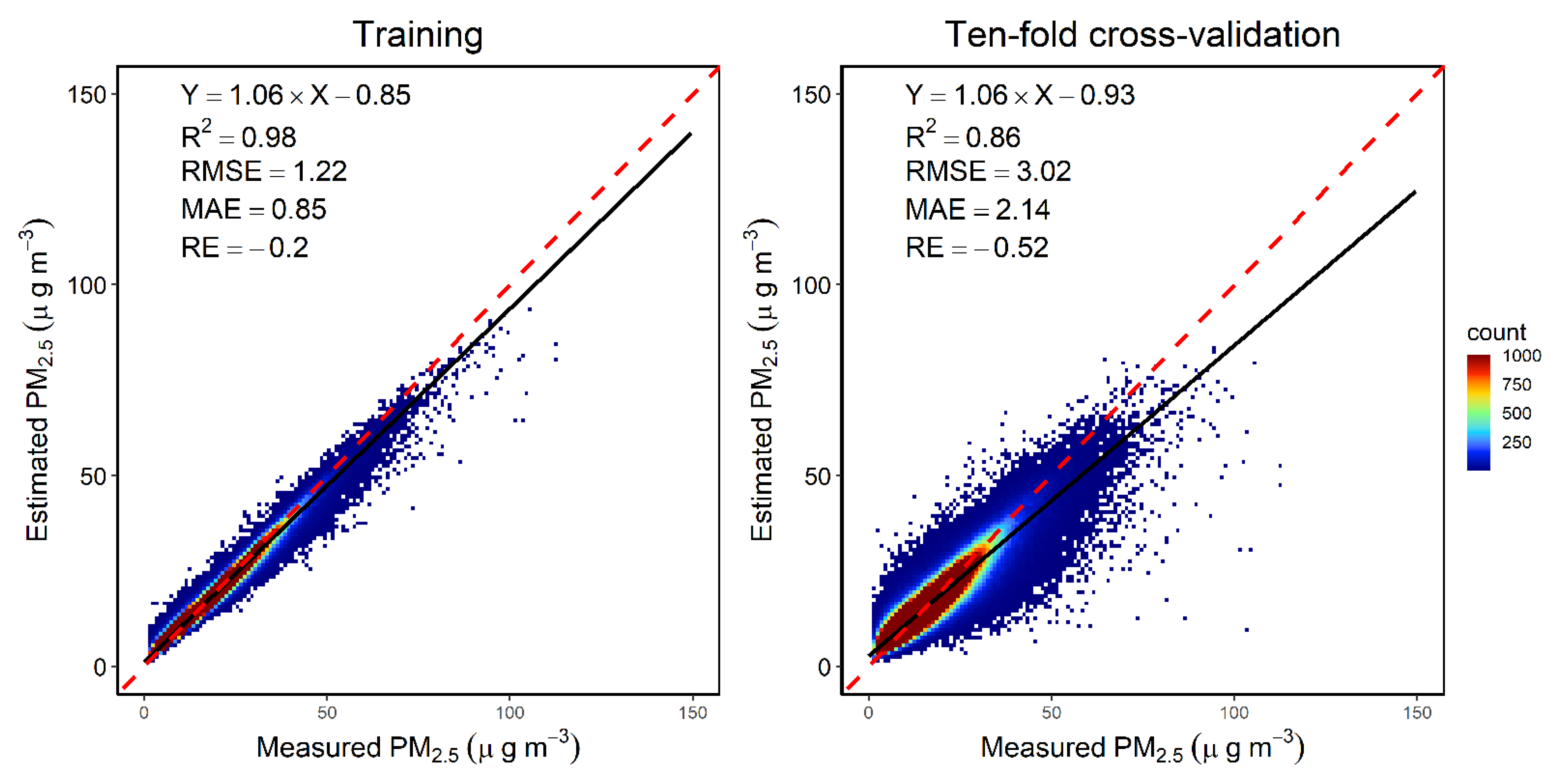
3.3. Model Performance of the First-Stage Model
3.4. Model Performance of the Second-Stage Model
3.5. Important Predictors of PM2.5 Concentrations
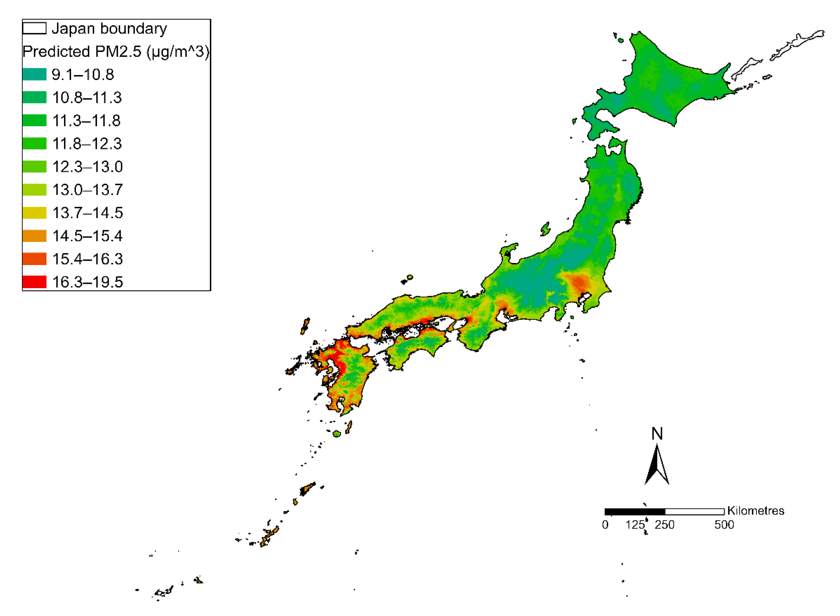
3.6. PM2.5 Estimates
4. Discussion
5. Conclusions
Supplementary Materials
Author Contributions
Funding
Institutional Review Board Statement
Data Availability Statement
Acknowledgments
Conflicts of Interest
References
- US EPA Particulate Matter (PM) Basics. Available online: https://www.epa.gov/pm-pollution/particulate-matter-pm-basics (accessed on 12 September 2021).
- Kim, K.H.; Kabir, E.; Kabir, S. A review on the human health impact of airborne particulate matter. Environ. Int. 2015, 74, 136–143. [Google Scholar] [CrossRef]
- Lin, Y.T.; Shih, H.; Jung, C.R.; Wang, C.M.; Chang, Y.C.; Hsieh, C.Y.; Hwang, B.F. Effect of exposure to fine particulate matter during pregnancy and infancy on paediatric allergic rhinitis. Thorax 2021, 76, 568–574. [Google Scholar] [CrossRef] [PubMed]
- Jung, C.R.; Chen, W.T.; Tang, Y.H.; Hwang, B.F. Fine particulate matter exposure during pregnancy and infancy and incident asthma. J. Allergy Clin. Immunol. 2019, 143, 2254–2262. [Google Scholar] [CrossRef] [PubMed]
- Alexeeff, S.E.; Liao, N.S.; Liu, X.; Van DenEeden, S.K.; Sidney, S. Long-term PM2.5 exposure and risks of ischemic heart disease and stroke events: Review and meta-analysis. J. Am. Heart Assoc. 2021, 10, 1–22. [Google Scholar] [CrossRef] [PubMed]
- Tsai, T.-L.; Lin, Y.-T.; Hwang, B.-F.; Nakayama, S.F.; Tsai, C.-H.; Sun, X.-L.; Ma, C.; Jung, C.-R. Fine particulate matter is a potential determinant of Alzheimer’s disease: A systemic review and meta-analysis. Environ. Res. 2019, 177, 108638. [Google Scholar] [CrossRef] [PubMed]
- Shi, L.; Zanobetti, A.; Kloog, I.; Coull, B.A.; Koutrakis, P.; Melly, S.J.; Schwartz, J.D. Low-concentration PM2.5 and mortality: Estimating acute and chronic effects in a population-based study. Environ. Health Perspect. 2016, 124, 46–52. [Google Scholar] [CrossRef] [Green Version]
- Li, P.; Sato, K.; Hasegawa, H.; Huo, M.; Minoura, H.; Inomata, Y.; Take, N.; Yuba, A.; Futami, M.; Takahashi, T.; et al. Chemical Characteristics and Source Apportionment of PM2.5 and Long-Range Transport from Northeast Asia Continent to Niigata in Eastern Japan. Aerosol Air Qual. Res. 2018, 18, 938–956. [Google Scholar] [CrossRef]
- Shimadera, H.; Kojima, T.; Kondo, A. Evaluation of Air Quality Model Performance for Simulating Long-Range Transport and Local Pollution of PM2.5 in Japan. Adv. Meteorol. 2016, 2016. [Google Scholar] [CrossRef] [Green Version]
- Eeftens, M.; Beelen, R.; Hoogh, K.d.; Bellander, T.; Cesaroni, G.; Cirach, M.; Declercq, C.; Dėdelė, A.; Dons, E.; Nazelle, A.d.; et al. Development of Land Use Regression Models for PM2.5, PM2.5 Absorbance, PM10 and PMcoarse in 20 European Study Areas; Results of the ESCAPE Project. Environ. Sci. Technol. 2012, 46, 11195–11205. [Google Scholar] [CrossRef]
- Gupta, P.; Christopher, S.A.; Wang, J.; Gehrig, R.; Lee, Y.; Kumar, N. Satellite remote sensing of particulate matter and air quality assessment over global cities. Atmos. Environ. 2006, 40, 5880–5892. [Google Scholar] [CrossRef]
- Xu, X.; Zhang, C.; Liang, Y. Review of satellite-driven statistical models PM2.5 concentration estimation with comprehensive information. Atmos. Environ. 2021, 256, 118302. [Google Scholar] [CrossRef]
- Kloog, I.; Koutrakis, P.; Coull, B.A.; Lee, H.J.; Schwartz, J. Assessing temporally and spatially resolved PM2.5exposures for epidemiological studies using satellite aerosol optical depth measurements. Atmos. Environ. 2011, 45, 6267–6275. [Google Scholar] [CrossRef]
- Hu, X.; Belle, J.H.; Meng, X.; Wildani, A.; Waller, L.A.; Strickland, M.J.; Liu, Y. Estimating PM2.5 Concentrations in the Conterminous United States Using the Random Forest Approach. Environ. Sci. Technol. 2017, 51, 6936–6944. [Google Scholar] [CrossRef]
- Hu, X.; Waller, L.A.; Lyapustin, A.; Wang, Y.; Al-Hamdan, M.Z.; Crosson, W.L.; Estes, M.G.; Estes, S.M.; Quattrochi, D.A.; Puttaswamy, S.J.; et al. Estimating ground-level PM2.5 concentrations in the Southeastern United States using MAIAC AOD retrievals and a two-stage model. Remote Sens. Environ. 2014, 140, 220–232. [Google Scholar] [CrossRef]
- Beloconi, A.; Chrysoulakis, N.; Lyapustin, A.; Utzinger, J.; Vounatsou, P. Bayesian geostatistical modelling of PM10 and PM2.5 surface level concentrations in Europe using high-resolution satellite-derived products. Environ. Int. 2018, 121, 57–70. [Google Scholar] [CrossRef]
- Shtein, A.; Kloog, I.; Schwartz, J.; Silibello, C.; Michelozzi, P.; Gariazzo, C.; Viegi, G.; Forastiere, F.; Karnieli, A.; Just, A.C.; et al. Estimating Daily PM2.5 and PM10 over Italy Using an Ensemble Model. Environ. Sci. Technol. 2020, 54, 120–128. [Google Scholar] [CrossRef]
- Xie, Y.; Wang, Y.; Zhang, K.; Dong, W.; Lv, B.; Bai, Y. Daily Estimation of Ground-Level PM2.5 Concentrations over Beijing Using 3 km Resolution MODIS AOD. Environ. Sci. Technol. 2015, 49, 12280–12288. [Google Scholar] [CrossRef] [PubMed] [Green Version]
- Xiao, Q.; Wang, Y.; Chang, H.H.; Meng, X.; Geng, G.; Lyapustin, A.; Liu, Y. Full-coverage high-resolution daily PM2.5 estimation using MAIAC AOD in the Yangtze River Delta of China. Remote Sens. Environ. 2017, 199, 437–446. [Google Scholar] [CrossRef]
- You, W.; Zang, Z.; Zhang, L.; Li, Y.; Pan, X.; Wang, W. National-scale estimates of ground-level PM2.5 concentration in China using geographically weighted regression based on 3 km resolution MODIS AOD. Remote Sens. 2016, 8, 184. [Google Scholar] [CrossRef] [Green Version]
- Yang, L.; Xu, H.; Jin, Z. Estimating ground-level PM2.5 over a coastal region of China using satellite AOD and a combined model. J. Clean. Prod. 2019, 227, 472–482. [Google Scholar] [CrossRef]
- Schneider, R.; Vicedo-Cabrera, A.M.; Sera, F.; Masselot, P.; Stafoggia, M.; deHoogh, K.; Kloog, I.; Reis, S.; Vieno, M.; Gasparrini, A. A satellite-based spatio-temporal machine learning model to reconstruct daily PM2.5 concentrations across great britain. Remote Sens. 2020, 12, 3803. [Google Scholar] [CrossRef] [PubMed]
- Jung, C.R.; Hwang, B.F.; Chen, W.T. Incorporating long-term satellite-based aerosol optical depth, localized land use data, and meteorological variables to estimate ground-level PM2.5 concentrations in Taiwan from 2005 to 2015. Environ. Pollut. 2018, 237, 1000–1010. [Google Scholar] [CrossRef] [PubMed]
- Levy, R.C.; Mattoo, S.; Munchak, L.A.; Remer, L.A.; Sayer, A.M.; Patadia, F.; Hsu, N.C. The Collection 6 MODIS aerosol products over land and ocean. Atmos. Meas. Tech. 2013, 6, 2989–3034. [Google Scholar] [CrossRef] [Green Version]
- Lyapustin, A.; Wang, Y.; Korkin, S.; Huang, D. MODIS Collection 6 MAIAC algorithm. Atmos. Meas. Tech. 2018, 11, 5741–5765. [Google Scholar] [CrossRef] [Green Version]
- Chu, Y.; Liu, Y.; Li, X.; Liu, Z.; Lu, H.; Lu, Y.; Mao, Z.; Chen, X.; Li, N.; Ren, M.; et al. A review on predicting ground PM2.5 concentration using satellite aerosol optical depth. Atmosphere 2016, 7, 129. [Google Scholar] [CrossRef] [Green Version]
- Brokamp, C.; Jandarov, R.; Hossain, M.; Ryan, P. Predicting Daily Urban Fine Particulate Matter Concentrations Using a Random Forest Model. Environ. Sci. Technol. 2018, 52, 4173–4179. [Google Scholar] [CrossRef]
- Zhang, T.; He, W.; Zheng, H.; Cui, Y.; Song, H.; Fu, S. Satellite-based ground PM2.5 estimation using a gradient boosting decision tree. Chemosphere 2021, 268, 128801. [Google Scholar] [CrossRef]
- Chen, Z.Y.; Zhang, T.H.; Zhang, R.; Zhu, Z.M.; Yang, J.; Chen, P.Y.; Ou, C.Q.; Guo, Y. Extreme gradient boosting model to estimate PM2.5 concentrations with missing-filled satellite data in China. Atmos. Environ. 2019, 202, 180–189. [Google Scholar] [CrossRef]
- Di, Q.; Kloog, I.; Koutrakis, P.; Lyapustin, A.; Wang, Y.; Schwartz, J. Assessing PM2.5 Exposures with High Spatiotemporal Resolution across the Continental United States. Environ. Sci. Technol. 2016, 50, 4712–4721. [Google Scholar] [CrossRef] [PubMed] [Green Version]
- Wang, X.; Sun, W. Meteorological parameters and gaseous pollutant concentrations as predictors of daily continuous PM2.5 concentrations using deep neural network in Beijing–Tianjin–Hebei, China. Atmos. Environ. 2019, 211, 128–137. [Google Scholar] [CrossRef]
- BCJ Japan Third Mesh Data. Available online: http://www.biodic.go.jp/kiso/col_mesh.html (accessed on 13 August 2020).
- Goddard Space Flight Center Aeronet-Aerosol Robotic Network. Available online: https://aeronet.gsfc.nasa.gov/ (accessed on 12 September 2021).
- Sayer, A.M.; Hsu, N.C.; Bettenhausen, C.; Jeong, M.J. Validation and uncertainty estimates for MODIS Collection 6 “deep Blue” aerosol data. J. Geophys. Res. Atmos. 2013, 118, 7864–7872. [Google Scholar] [CrossRef] [Green Version]
- NIES Environment Numerical Database. Available online: https://www.nies.go.jp/igreen/index.html (accessed on 13 August 2020).
- Japan Meteorological Agency AMeDAS. Available online: https://www.jma.go.jp/jma/en/Activities/amedas/amedas.html (accessed on 1 June 2021).
- Araki, S.; Yamamoto, K.; Kondo, A. Application of Regression Kriging to Air Pollutant Concentrations in Japan with High Spatial Resolution. Aerosol Air Qual. Res. 2015, 15, 234–241. [Google Scholar] [CrossRef] [Green Version]
- Chen, X.; Ding, J.; Liu, J.; Wang, J.; Ge, X.; Wang, R.; Zuo, H. Validation and comparison of high-resolution MAIAC aerosol products over Central Asia. Atmos. Environ. 2021, 251, 118273. [Google Scholar] [CrossRef]
- She, L.; Zhang, H.; Wang, W.; Wang, Y.; Shi, Y. Evaluation of the Multi-Angle Implementation of Atmospheric Correction (MAIAC) Aerosol Algorithm for Himawari-8 Data. Remote Sens. 2019, 11, 2771. [Google Scholar] [CrossRef] [Green Version]
- Liaw, A.; Wiener, M. Classification and Regression by randomForest. R News 2002, 2, 18–22. [Google Scholar]
- James, G.; Witten, D.; Hastie, T.; Tibshirani, R. An introduction to Statistical Learning with Application in R.; Springer Nature: New York, NY, USA, 2013. [Google Scholar]
- Wang, C.M.; Jung, C.R.; Chen, W.T.; Hwang, B.F. Exposure to fine particulate matter (PM2.5) and pediatric rheumatic diseases. Environ. Int. 2020, 138, 105602. [Google Scholar] [CrossRef] [PubMed]
- Kloog, I.; Sorek-Hamer, M.; Lyapustin, A.; Coull, B.; Wang, Y.; Just, A.C.; Schwartz, J.; Broday, D.M. Estimating daily PM2.5 and PM10 across the complex geo-climate region of Israel using MAIAC satellite-based AOD data. Atmos. Environ. 2015, 122, 409–416. [Google Scholar] [CrossRef] [PubMed] [Green Version]
- Chen, Z.; Chen, D.; Zhao, C.; Kwan, M.; Cai, J.; Zhuang, Y.; Zhao, B.; Wang, X.; Chen, B.; Yang, J.; et al. Influence of meteorological conditions on PM2.5 concentrations across China: A review of methodology and mechanism. Environ. Int. 2020, 139, 105558. [Google Scholar] [CrossRef]
- Chen, T.; Guestrin, C. XGBoost: A scalable tree boosting system. In Proceedings of the ACM SIGKDD International Conference on Knowledge Discovery and Data Mining, San Francisco, CA, USA, 13–17 August 2016; pp. 785–794. [Google Scholar]
- Araki, S.; Shima, M.; Yamamoto, K. Estimating historical PM2.5 exposures for three decades (1987–2016) in Japan using measurements of associated air pollutants and land use regression. Environ. Pollut. 2020, 263, 114476. [Google Scholar] [CrossRef]
- Mhawish, A.; Banerjee, T.; Sorek-Hamer, M.; Lyapustin, A.; Broday, D.M.; Chatfield, R. Comparison and evaluation of MODIS Multi-angle Implementation of Atmospheric Correction (MAIAC) aerosol product over South Asia. Remote Sens. Environ. 2019, 224, 12–28. [Google Scholar] [CrossRef]
- Zhang, Q.; Zheng, Y.; Tong, D.; Shao, M.; Wang, S.; Zhang, Y.; Xu, X.; Wang, J.; He, H.; Liu, W.; et al. Drivers of improved PM2.5 air quality in China from 2013 to 2017. Proc. Natl. Acad. Sci. USA 2019, 116, 24463–24469. [Google Scholar] [CrossRef] [Green Version]
- Araki, S.; Shimadera, H.; Yamamoto, K.; Kondo, A. Effect of spatial outliers on the regression modelling of air pollutant concentrations: A case study in Japan. Atmos. Environ. 2017, 153, 83–93. [Google Scholar] [CrossRef] [Green Version]
- Araki, S.; Hasunuma, H.; Yamamoto, K.; Shima, M.; Michikawa, T.; Nitta, H.; Nakayama, S.F.; Yamazaki, S. Estimating monthly concentrations of ambient key air pollutants in Japan during 2010–2015 for a national-scale birth cohort. Environ. Pollut. 2021, 284, 117483. [Google Scholar] [CrossRef]
- Chen, W.; Ran, H.; Cao, X.; Wang, J.; Teng, D.; Chen, J.; Zheng, X. Estimating PM2.5 with high-resolution 1-km AOD data and an improved machine learning model over Shenzhen, China. Sci. Total Environ. 2020, 746, 141093. [Google Scholar] [CrossRef]
- Stafoggia, M.; Bellander, T.; Bucci, S.; Davoli, M.; Hoogh, K.d.; Donato, F.d.; Gariazzo, C.; Lyapustin, A.; Michelozzi, P.; Renzi, M.; et al. Estimation of daily PM10 and PM2.5 concentrations in Italy, 2013–2015, using a spatiotemporal land-use random-forest model. Environ. Int. 2019, 124, 170–179. [Google Scholar] [CrossRef]
- Zhang, R.; Di, B.; Luo, Y.; Deng, X.; Grieneisen, M.L.; Wang, Z.; Yao, G.; Zhan, Y. A nonparametric approach to filling gaps in satellite-retrieved aerosol optical depth for estimating ambient PM2.5 levels. Environ. Pollut. 2018, 243, 998–1007. [Google Scholar] [CrossRef] [PubMed]
- Coulibaly, S.; Minami, H.; Abe, M.; Hasei, T.; Sera, N.; Yamamoto, S.; Funasaka, K.; Asakawa, D.; Watanabe, M.; Honda, N.; et al. Seasonal Fluctuations in Air Pollution in Dazaifu, Japan, and Effect of Long-Range Transport from Mainland East Asia. Biol. Pharm. Bull. 2015, 38, 1395–1403. [Google Scholar] [CrossRef] [Green Version]
- Nakata, M.; Sano, I.; Mukai, S. Air pollutants in Osaka (Japan). Front. Environ. Sci. 2015, 3, 18. [Google Scholar] [CrossRef] [Green Version]
- Joharestani, M.Z.; Cao, C.; Ni, X.; Bashir, B.; Talebiesfandarani, S. PM2.5 Prediction Based on Random Forest, XGBoost, and Deep Learning Using Multisource Remote Sensing Data. Atmosphere 2019, 10, 373. [Google Scholar] [CrossRef] [Green Version]
- Engel-Cox, J.A.; Holloman, C.H.; Coutant, B.W.; Hoff, R.M. Qualitative and quantitative evaluation of MODIS satellite sensor data for regional and urban scale air quality. Atmos. Environ. 2004, 38, 2495–2509. [Google Scholar] [CrossRef]
- Wang, J.; Ogawa, S. Effects of Meteorological Conditions on PM2.5 Concentrations in Nagasaki, Japan. Int. J. Environ. Res. Public Health 2015, 12, 9089–9101. [Google Scholar] [CrossRef] [PubMed]
- Tsai, T.C.; Jeng, Y.J.; Chu, D.A.; Chen, J.P.; Chang, S.C. Analysis of the relationship between MODIS aerosol optical depth and particulate matter from 2006 to 2008. Atmos. Environ. 2011, 45, 4777–4788. [Google Scholar] [CrossRef]
- Just, A.C.; Wright, R.O.; Schwartz, J.; Coull, B.A.; Baccarelli, A.A.; Tellez-Rojo, M.M.; Moody, E.; Wang, Y.; Lyapustin, A.; Kloog, I. Using High-Resolution Satellite Aerosol Optical Depth To Estimate Daily PM2.5 Geographical Distribution in Mexico City. Environ. Sci. Technol. 2015, 49, 8576–8584. [Google Scholar] [CrossRef] [PubMed] [Green Version]
- Lv, B.; Hu, Y.; Chang, H.H.; Russell, A.G.; Bai, Y. Improving the Accuracy of Daily PM2.5 Distributions Derived from the Fusion of Ground-Level Measurements with Aerosol Optical Depth Observations, a Case Study in North China. Environ. Sci. Technol. 2016, 50, 4752–4759. [Google Scholar] [CrossRef] [PubMed]
- Michikawa, T.; Nitta, H.; Nakayama, S.F.; Yamazaki, S.; Isobe, T.; Tamura, K.; Suda, E.; Ono, M.; Yonemoto, J.; Iwai-Shimada, M.; et al. Baseline Profile of Participants in the Japan Environment and Children’s Study (JECS). J. Epidemiol. 2018, 28, 99–104. [Google Scholar] [CrossRef] [Green Version]
- Yang, J.; Hu, M. Filling the missing data gaps of daily MODIS AOD using spatiotemporal interpolation. Sci. Total Environ. 2018, 633, 677–683. [Google Scholar] [CrossRef]
- Chen, G.; Li, S.; Knibbs, L.D.; Hamm, N.A.S.; Cao, W.; Li, T.; Guo, J.; Ren, H.; Abramson, M.J.; Guo, Y. A machine learning method to estimate PM2.5 concentrations across China with remote sensing, meteorological and land use information. Sci. Total Environ. 2018, 636, 52–60. [Google Scholar] [CrossRef] [PubMed]
- Huang, K.; Xiao, Q.; Meng, X.; Geng, G.; Wang, Y.; Lyapustin, A.; Gu, D.; Liu, Y. Predicting monthly high-resolution PM2.5 concentrations with random forest model in the North China Plain. Environ. Pollut. 2018, 242, 675–683. [Google Scholar] [CrossRef]


| Period | Number | Mean | SD | Min | Q1 | Median | Q3 | Max | IQR |
|---|---|---|---|---|---|---|---|---|---|
| Overall | 1,491,808 | 14.3 | 8.1 | 0.0 | 8.4 | 12.5 | 18.2 | 149.5 | 9.8 |
| Spring | 378,303 | 16.6 | 8.5 | 0.0 | 10.6 | 15.2 | 20.9 | 112.5 | 10.3 |
| Summer | 362,641 | 14.8 | 8.4 | 0.0 | 8.7 | 12.9 | 18.9 | 101.0 | 10.2 |
| Autumn | 368,560 | 12.8 | 6.8 | 0.0 | 7.9 | 11.5 | 16.2 | 97.2 | 8.3 |
| Winter | 382,304 | 12.8 | 7.8 | 0.0 | 7.3 | 10.8 | 16.3 | 149.5 | 9.0 |
| Period | Number a | Mean | SD | Min | Q1 | Median | Q3 | Max | IQR |
|---|---|---|---|---|---|---|---|---|---|
| Overall | 129,090,082 (15.48%) | 0.182 | 0.145 | 0 | 0.091 | 0.145 | 0.231 | 3.770 | 0.140 |
| Spring | 37,531,792 (17.94%) | 0.264 | 0.182 | 0 | 0.148 | 0.226 | 0.330 | 3.180 | 0.182 |
| Summer | 22,073,935 (10.51%) | 0.206 | 0.158 | 0 | 0.107 | 0.170 | 0.263 | 3.773 | 0.156 |
| Autumn | 40,183,589 (19.49%) | 0.128 | 0.079 | 0 | 0.074 | 0.111 | 0.163 | 3.516 | 0.089 |
| Winter | 29,300,766 (14.05%) | 0.134 | 0.087 | 0 | 0.076 | 0.115 | 0.170 | 1.750 | 0.094 |
| Period | Number | Mean | SD | Min | Q1 | Median | Q3 | Max | IQR |
|---|---|---|---|---|---|---|---|---|---|
| Overall | 832,177,456 | 12.5 | 5.5 | 1.2 | 8.8 | 11.4 | 15.0 | 93.6 | 6.2 |
| Spring | 209,562,936 | 14.7 | 6.0 | 1.2 | 10.6 | 13.6 | 17.3 | 93.6 | 6.7 |
| Summer | 209,562,936 | 13.2 | 5.5 | 1.3 | 9.4 | 12.2 | 15.8 | 69.6 | 6.4 |
| Autumn | 207,285,078 | 11.1 | 4.6 | 1.4 | 8.0 | 10.1 | 13.0 | 77.0 | 5.0 |
| Winter | 205,766,506 | 11.1 | 4.8 | 1.4 | 7.9 | 10.1 | 13.0 | 88.1 | 5.1 |
Publisher’s Note: MDPI stays neutral with regard to jurisdictional claims in published maps and institutional affiliations. |
© 2021 by the authors. Licensee MDPI, Basel, Switzerland. This article is an open access article distributed under the terms and conditions of the Creative Commons Attribution (CC BY) license (https://creativecommons.org/licenses/by/4.0/).
Share and Cite
Jung, C.-R.; Chen, W.-T.; Nakayama, S.F. A National-Scale 1-km Resolution PM2.5 Estimation Model over Japan Using MAIAC AOD and a Two-Stage Random Forest Model. Remote Sens. 2021, 13, 3657. https://doi.org/10.3390/rs13183657
Jung C-R, Chen W-T, Nakayama SF. A National-Scale 1-km Resolution PM2.5 Estimation Model over Japan Using MAIAC AOD and a Two-Stage Random Forest Model. Remote Sensing. 2021; 13(18):3657. https://doi.org/10.3390/rs13183657
Chicago/Turabian StyleJung, Chau-Ren, Wei-Ting Chen, and Shoji F. Nakayama. 2021. "A National-Scale 1-km Resolution PM2.5 Estimation Model over Japan Using MAIAC AOD and a Two-Stage Random Forest Model" Remote Sensing 13, no. 18: 3657. https://doi.org/10.3390/rs13183657
APA StyleJung, C.-R., Chen, W.-T., & Nakayama, S. F. (2021). A National-Scale 1-km Resolution PM2.5 Estimation Model over Japan Using MAIAC AOD and a Two-Stage Random Forest Model. Remote Sensing, 13(18), 3657. https://doi.org/10.3390/rs13183657