Assessment of Empirical and Semi-Analytical Algorithms Using MODIS-Aqua for Representing In-Situ Chromophoric Dissolved Organic Matter (CDOM) in the Bering, Chukchi, and Western Beaufort Seas of the Pacific Arctic Region

Abstract

We analyzed a variety of satellite-based ocean color products derived using MODIS-Aqua to investigate the most accurate empirical and semi-analytical algorithms for representing in-situ chromophoric dissolved organic matter (CDOM) across a large latitudinal transect in the Bering, Chukchi, and western Beaufort Seas of the Pacific Arctic region. In particular, we compared the performance of empirical (CDOM index) and several semi-analytical algorithms (quasi-analytical algorithm (QAA), Carder, Garver-Siegel-Maritorena (GSM), and GSM-A) with field measurements of CDOM absorption (a_CDOM) at 412 nanometers (nm) and 443 nm. These algorithms were compared with in-situ CDOM measurements collected on cruises during July 2011, 2013, 2014, 2015, 2016, and 2017. Our findings show that the QAA a443 and GSM-A a443 algorithms are the most accurate and robust representation of in-situ conditions, and that the GSM-A a443 algorithm is the most accurate algorithm when considering all statistical metrics utilized here. Our further assessments indicate that geographic variables (distance to coast, latitude, and sampling transects) did not obviously relate to algorithm accuracy. In general, none of the algorithms investigated showed a statistically significant agreement with field measurements beyond an approximately ± 60 h offset, likely owing to the highly variable environmental conditions found across the Pacific Arctic region. As such, we suggest that satellite observations of CDOM in these Arctic regions should not be used to represent in-situ conditions beyond a ± 60 h timeframe.

1. Introduction

Chromophoric dissolved organic matter (CDOM) represents the optical fraction of dissolved organic matter in natural waters, and its production impacts the heating and propagation of light in the water column [1]. As climate change continues, variability in CDOM distribution may have major effects on primary production and carbon cycling in the Arctic Ocean, particularly in the Bering, Chukchi, and western Beaufort Seas of the Pacific Arctic region. CDOM will further shift in coastal areas as anthropogenic eutrophication occurs owing to changes in continental runoff, atmospheric nutrient deposition, and ocean warming [2,3]. Another major factor influencing CDOM production and distribution is sea-ice extent. The Pacific Arctic region, in particular, is undergoing the greatest seasonal sea-ice thinning and retreat of the entire Arctic region [4,5,6,7]. Less sea ice and more melt ponds lead to increases in: (a) light availability in the water column [8], (b) primary production (e.g., photosynthesis and phytoplankton production) [9,10], (c) autochthonous CDOM (i.e., produced through phytoplankton decay), and (d) allochthonous CDOM (i.e., formed on land and transported through riverine inputs to coastal areas) [1,11,12]. As such, all of these dynamics create complexities in CDOM production, distribution, and measurements across this region.

The remoteness of this area and the limitation of seasonal in-situ measurements require other tools, such as satellite instruments, to monitor the spatial and temporal distribution of CDOM. Indeed, the optical properties of CDOM allow for monitoring by ocean color satellite instruments during summer months after the sea-ice melt season. Satellite measurements by the Moderate Resolution Imaging Spectroradiometer onboard Aqua (MODIS-Aqua) provide important estimates of CDOM in surface waters. Current ocean color CDOM algorithms work most efficiently for retrieval in open ocean or Case-1 waters from a global in-situ data set in which CDOM production is minimal [13]. However, most currently available CDOM algorithms do not take into consideration other variations of CDOM production from both autochthonous and allochthonous sources in a regional area, such as in the Bering, Chukchi, and Beaufort Seas. Optically complex waters have variable concentrations of CDOM, chlorophyll-a (chl-a), and total suspended matter that can contribute to challenges associated with the retrieval of all of these parameters (including CDOM) when using satellite remote sensing [14]. CDOM is detected by satellites using a combination of empirical (e.g., band ratio) and semi-analytical algorithms in which CDOM is estimated at four distinctive wavelengths (412, 443, 490, and 555 nm) [15,16]. Empirical algorithms (e.g., R(412)/R(443) and R(490)/R(555)) are commonly used for spectral and/or surface reflectance (R) in open ocean waters [11]. The ratio between R(412)/R(443) is sensitive to CDOM, while the ratio for R(490)/R(555) depends on chl-a, which is also influenced by CDOM. However, empirical algorithms can under- or overestimate CDOM production because of other bio-optical signatures or factors, such as the presence of phytoplankton and detrital material, which are ubiquitously found in natural waters. Variations in these ratios may be established via bio-optical models developed for Case-1 instead of Case-2 (i.e., coastal) waters. On the other hand, semi-analytical algorithms [17] and quasi-analytical algorithms (QAA) [18,19] have also been utilized to remotely retrieve CDOM. Semi-analytical algorithms and QAA do allow for the incorporation of phytoplankton and detrital material into calculations. This can also lead to overestimation, but these algorithms are still considered more accurate than empirical algorithms because they can more robustly depict environmental conditions found in the field.

A number of studies have used satellite measurements, including MODIS-Aqua, to retrieve CDOM using empirical and/or semi-analytical algorithms in Case-1 waters. Empirical algorithms, such as the CDOM index, were developed as band ratios at four wavelengths, including R_rs(412)/R_rs(443) and R_rs(490)/R_rs(555), to retrieve CDOM and chl-a concentrations in mostly oceanic waters [16]. Other empirical algorithms were recently compared to in-situ data collected in the summer of 2010 and 2011 as part of the NASA Impacts of Climate Change on the Eco-Systems and Chemistry of the Arctic Pacific Environment (ICESCAPE) mission in the western Arctic [20]. Those authors reported that there were overestimates for the empirical algorithms used to retrieve chl-a when compared to in-situ measurements. Furthermore, another linear empirical algorithm (OC3L) was recently developed to improve ocean color empirical algorithms (e.g., OC3Mv6) in the western Arctic Ocean, also as part of the NASA ICESCAPE mission [21]. Those authors presented a three-band input, R(443) > R(490)/R(555), to retrieve chl-a, and consequently to reduce statistical error from CDOM in the Chukchi Sea. That empirical algorithm was calibrated with coincident in-situ measurements for both chl-a and CDOM [21]. However, retrieving CDOM measurements under highly variable environmental conditions across a large latitudinal area may still be challenging.

In contrast to the band ratio algorithms, semi-analytical algorithms are considered more reliable since different oceanic constituents, such as chl-a, phytoplankton absorption, and particulate backscattering, are retrieved and analyzed concurrently in surface waters [22]. The QAA and Carder algorithms each combine measured remote sensing surface reflectance (R_rs (λ)) as well as theoretical and empirical models yielding a set of simultaneous equations to retrieve chl-a in the presence of CDOM [18,19,23]. In addition, the Garver-Siegel-Maritorena (GSM) model combines R_rs (λ), backscatter and absorption coefficients with empirical formulas to retrieve CDOM, chl-a concentration, and the particulate backscatter coefficient in clear waters [17,24]. More recently, the GSM-A semi-analytical algorithm was created for use in Case-1 and Case-2 Arctic waters [25,26]. The GSM-A was designed specifically for the western Beaufort Sea; two factors, including the presence of sea-ice and large quantities of terrigenous CDOM transported to coastal areas, need to be present to retrieve CDOM accurately for this particular algorithm.

The objective of this study was to compare satellite measurements with in-situ measurements of CDOM collected in July 2011, 2013, 2014, 2015, 2016, and 2017 for CDOM across the Pacific Arctic region. We compared empirical and semi-analytical algorithms, including Carder, QAA, GSM, GSM-A, and CDOM index for the absorption of CDOM absorption a_CDOM at 412 nm and 443 nm across our study region. Statistical analyses were performed using Pearson’s correlation coefficient (R), mean deviation (MD), mean absolute deviation (MAD), slope of the least squares, mean percent deviation (MPD), and standard deviation to study how MODIS-Aqua satellite data compare to our in-situ measurements. This study provides a first simultaneous assessment of multiple satellite-based CDOM algorithms across the broad Pacific Arctic region using multiple years of in-situ observations. Moreover, we additionally present a first sensitivity study to better understand the time frame over which satellite-based CDOM algorithms represent field-based CDOM most accurately (i.e., over what time period do field and satellite measurements diverge from one another), providing insight into the temporal utility of these satellite observations that has not previously existed.

2. Materials and Methods

2.1. Study Area and CDOM Absorption

Ocean water samples were collected as part of the NASA-Impacts of Climate on the Eco-Systems and Chemistry of the Arctic Pacific Environment (ICESCAPE) mission on the U.S. Coast Guard Cutter (USCGC) Healy in July 2011 in the Chukchi and western Beaufort Seas as well as the NSF-Arctic Observing Network Distributed Biological Observatory (DBO) program [27] in July from 2013 to 2017 in the Bering and Chukchi Seas onboard the Canadian Coast Guard Ship Sir Wilfrid Laurier (SWL) (Figure 1). We collected seawater samples (for this study we used samples at the shallowest depth collected, at 5 m) using the CTD rosettes of the Healy and SWL research vessels, which consisted of a 12-place rosette with 30 L Niskin bottles and 24-place rosette with 10 L Niskin bottles, respectively. Collection vessels used were acid washed (10% HCl) and pre-combusted (450 °C for 6 h) foil-covered Kimax clear glass bottles. Immediately after collections, 125 mL of seawater was filtered using 0.2 μm Whatman Nuclepore polycarbonate filter (pre-soaked with 10% HCl and soaked/rinsed with Milli-Q) and analyzed for CDOM absorbance following filtering.

The analysis of CDOM was performed onboard the SWL research vessel for July 2013–2017. Filtered seawater samples were stored in the dark at 4 °C in acid washed (10% HCl) and pre-combusted (450 °C for 6 h) foil-covered Qorpak clear glass bottles. The caps were additionally pre-soaked (10% HCl), soaked/rinsed with Milli-Q, and air dried before using. The CDOM samples were analyzed within 24 h of collection (most typically within 1–2 h) onboard the SWL. For July 2011 on the Healy cruise, water samples were frozen after filtration owing to the ship’s ice-breaking activities and later analyzed onshore in the Polar Science Research Laboratory at Clark University. In both cases, CDOM was measured using a Shimadzu UV-1800 UV/Visible scanning spectrophotometer between wavelengths of 800 and 200 nm at 1-nm increments using a 10-cm cuvette and Milli-Q blank correction. Absorbance values were calculated as follows:

$$a_{\lambda }=2.303A_{\lambda }/I$$

(1)

where A_λ is the raw absorbance value from the spectrophotometer, a is the Naperian absorbance coefficient (m⁻¹) at a specific wavelength (λ), and I is the cell path length (m) [28]. Field-based CDOM data are available at the National Science Foundation Arctic Data Center (doi numbers are below in the Data Availability Statement).

2.2. Ocean Color Satellite Remote Sensing Data

MODIS-Aqua Level-1A files were downloaded from the NASA Ocean Biology Processing Group (OBPG) http://oceancolor.gsfc.nasa.gov (accessed from 20 December 2017 to 8 January 2018) for July 2011, 2013, 2014, 2015, 2016, and 2017. Geometric and atmospheric corrections were applied to Level-1A data, which included reconstructed and/or unprocessed instrument data at full resolution, and batch processed to Level-3 data (i.e., well-defined spatial grid, including binned and mapped, over a well-defined time period) using SeaDAS 7.5 and Python 2.7.15 [29]. Empirical and semi-analytical algorithms were then evaluated using remote sensing surface reflectance (R_rs) visible bands at 412 and 443 nm to analyze the performance of empirical and semi-analytical algorithms, including CDOM index R_rs(412)/R_rs(443) [16], QAA [18], Carder [23,30], GSM [17,24], and GSM-A (specific for Arctic waters) [25]. The R_rs for GSM-A at 412, 443, 488, 531, 555, and 678 nm were further calculated using RStudio version 1.1.447, RStudio, Boston, MA.

We did not change default values (e.g., chlorophyll-a, total suspended matter) in the existing algorithms in order to best assess the accuracy of the CDOM algorithms as they are widely available to the general public. That being said, the mean chlorophyll-a concentration of our ~5 m surface water samples (associated with our in-situ CDOM measurements) in this study was 1.354 mg/m³ (N = 170), which was in range of the default values in the assessed algorithms (0.002–10.00 mg/m³ for Carder [23], 0.07–49.40 mg/m³ for QAA [18], and 0.02–10.00 mg/m³ for GSM [17]). In the case of the GSM-A region, the geometric mean of summer chlorophyll-a concentrations was 0.553 mg/m³ [31], which was remarkably similar to the geometric mean of our surface water samples (0.53 mg/m³). Although chlorophyll-a concentrations in the Pacific Arctic region can be much higher during the spring/early-summer seasonal phytoplankton bloom, our consistent sampling later in the season during July (after this seasonal bloom) clearly allowed for more comparative values with existing CDOM algorithms and supported the acceptability of retaining default parameters.

Level-2 raster files (processed from the Level-1A data as above) were also utilized to compare CDOM MODIS-Aqua satellite measurements to in-situ measurements (in 2011, 2013, 2014, 2015, 2016, and 2017) using WimSoft WAM-match module version 10.09, http://www.wimsoft.com (accessed on 9 June 2018) [32]. The water column field measurements used for match-ups were collected at a ~5 m depth (the shallowest depth collected via CTD). Specifically, (a) the time lag was defined at a maximum of ±120 h, with the results binned into successive 12-h groupings for subsequent comparisons (e.g., ±12 h, ±24 h, ±36 h); (b) satellite values were filtered for unmasked pixels in a 5 × 5 box centered on the in-situ target; (c) a minimum of 13 was set for valid pixels (within the 5 × 5 window) to accept a matchup; and (d) the valid maximum and minimum values established were 64.5 and 0.016, respectively.

2.3. Statistical Analyses and Temporal Sensitivity Study

Pearson’s correlation coefficient (R), mean deviation (MD), mean absolute deviation (MAD), slope of the least squares, and average percent deviation (APD) were part of the broad statistical analyses to compare CDOM MODIS-Aqua satellite measurements with our field measurements. Our first step was to determine which of the 8 algorithms (GSM a412, GSM a443, QAA a412, QAA a443, Carder a412, Carder a443, CDOM Index, and GSM-A a443) and 10 different temporal offsets associated with each (±12, ±24, ±36, ±48, ±60, ±72, ±84, ±96, ±108, and ±120 h) showed statistically significant R values when comparing satellite with in-situ measurements. Using these methods, we performed a temporal sensitivity study to better understand the time frame over which satellite and in-situ observations began to diverge from one another, specifically over this 12 to 120-h timeframe (before and after the time of field collections). Next, for those relationships that showed statistically significant R values, we calculated MD and MAD to compare these resulting culled satellite-based algorithms (Y) with field measurements (X) [33]. These metrics are generally utilized to understand how points are distributed with respect to the Y = X (i.e., 1:1) line for a given relationship, where X and Y describe the same continuous phenomenon [33]. These statistics were calculated in linear space but plotted with a logarithmic scale. The MD was calculated to understand how the average deviation of values compared to the overall mean. The MAD was calculated to show the average vertical distance between the points with respect to the 1:1 line (using absolute values). Those values closest to 0 indicated relationships with the least dispersion from the 1:1 line of the satellite-field relationship. Next, the slope of the least squares line was calculated to provide additional insight for the proximity of the satellite-field relationship to the 1:1 line. Last, for those relationships that showed MD and MAD values closest to zero, we calculated and plotted the modal distribution of APD for each satellite-field match-up point.

3. Results

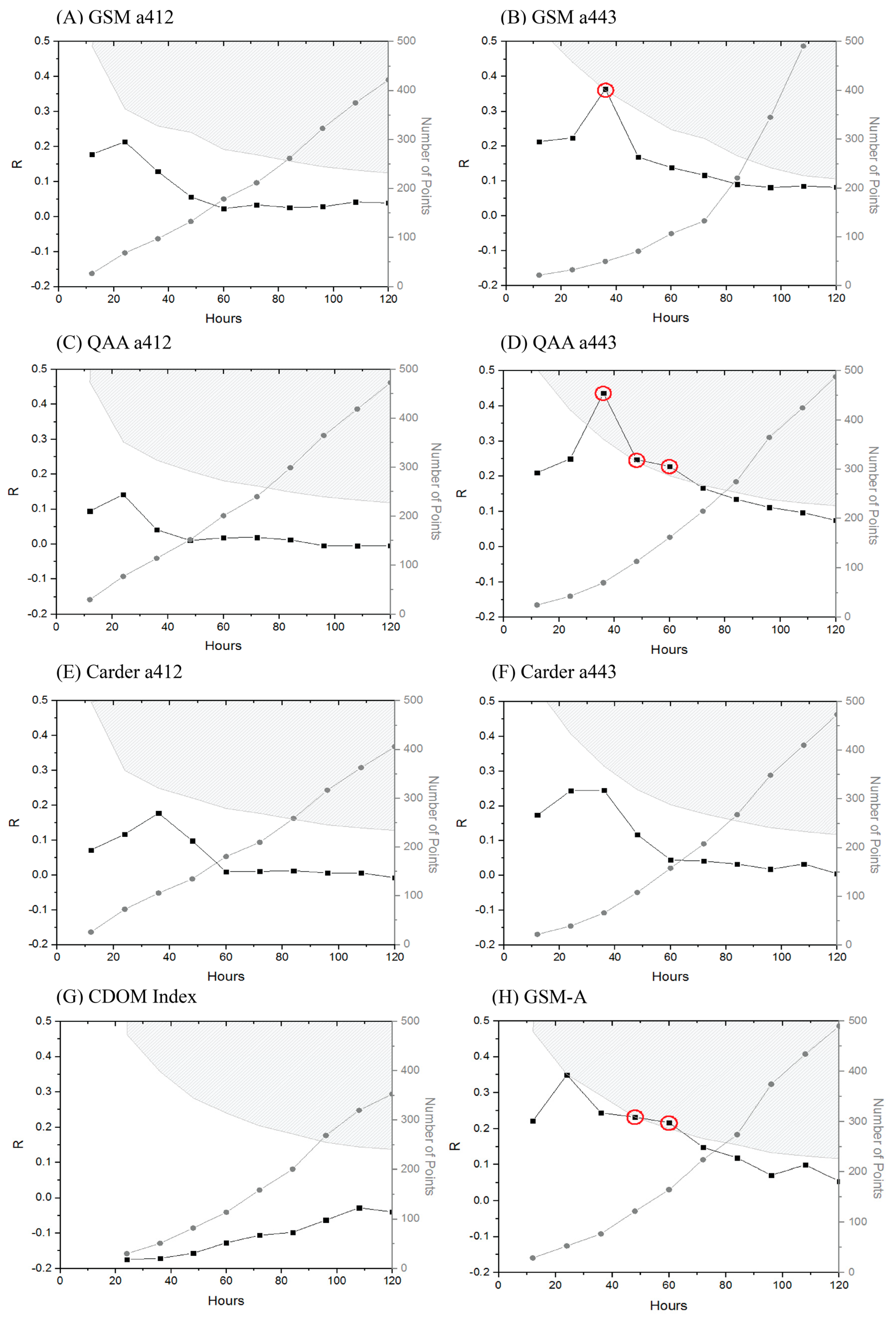
3.1. R Values for Temporal Sensitivity Study

We first performed a temporal sensitivity study to understand which CDOM MODIS-Aqua algorithm(s) best statistically aligned with our in-situ measurements (Figure 2). The tested algorithms included GSM a412 and a443, QAA a412 and a443, Carder a412 and a443, CDOM index, and GSM-A a443. The number of hours that each algorithm was tested was up to ±120 (i.e., both before and after the time of field collection); we included satellite comparisons with both the ICESCAPE samples taken in July 2011 and stations within the DBO sites 1–5 sampled in July 2013, 2014, 2015, 2016, and 2017 (Figure 1). The gray shaded areas show those R values that were statistically significant at p < 0.01 for each time step investigated (at 12-h increments). When the black squares fell within the gray shaded area, these squares were statistically significant (circled in red), and all others were not statistically significant.

The CDOM MODIS-Aqua GSM a412 algorithm did not have any statistically significant R values (Figure 2A), but the GSM a443 had one statistically significant R value that overlapped with the gray area at ±36 h (Figure 2B). Similarly, the QAA a412 algorithm did not have any significant R values; however, the QAA a443 algorithm had three significant R values (Figure 2C,D). The three significant R values were specifically at ±36, ±48, and ±60 h. This was not the case for the MODIS-Aqua Carder a412 and a443 (Figure 2E,F) and CDOM index (Figure 2G) algorithms, which had no statistically significant or overlapping points with the gray area. However, the GSM-A algorithm had two significant R values, which were at ±48 and ±60 h (Figure 2H). Each time step was associated with an N (number of points in our scatterplots, which we discuss in the next section), so those significant values of R (i.e., the gray shaded areas) were also based on degrees of freedom (N-2). N increased with time because there were more satellite overpasses available over longer stretches of time and that therefore had more in-situ match-ups (and hence the critical threshold for the R values (p < 0.01) decreased with time).

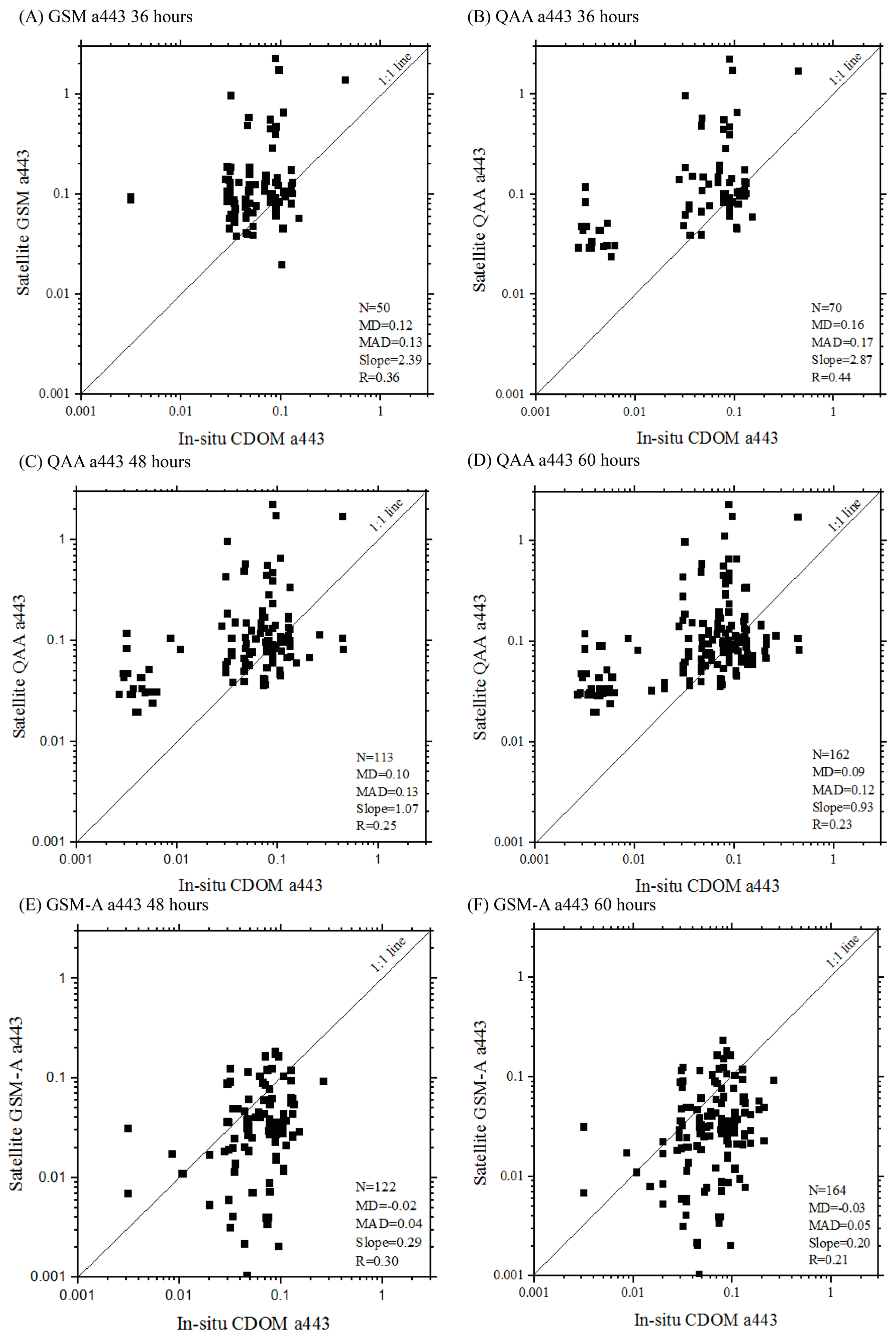
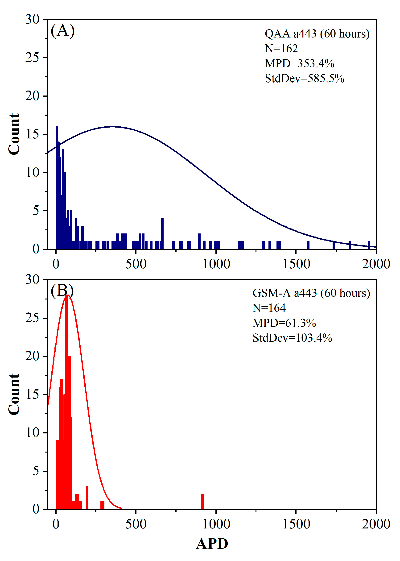
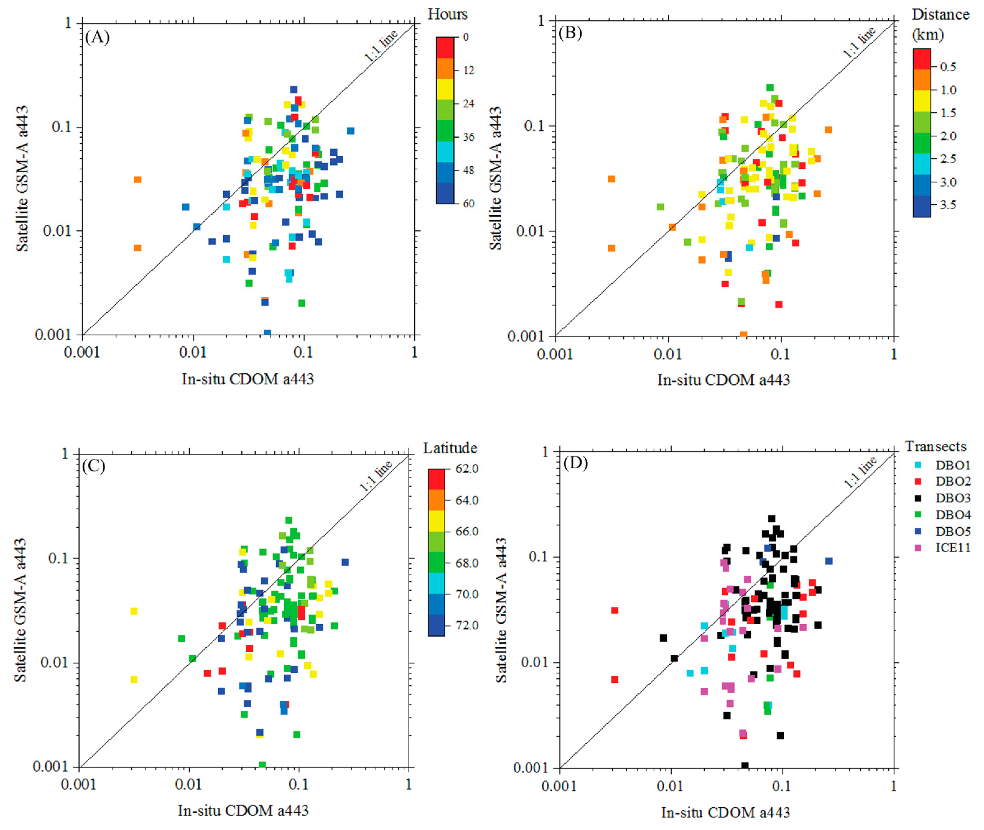
3.2. Statistically Significant CDOM Algorithms

There were only six situations where R values were statistically significant for the CDOM MODIS-Aqua algorithms (six varying time steps among three algorithms: GSM a443, QAA a443, and GSM-A a443) (Figure 2B,D,H), with the scatterplots associated with these algorithms and time steps (i.e., those circled in red in Figure 2) shown in Figure 3. These overall statistical results are summarized in

Table 1. Statistical summary for the six algorithms/time steps with the most significant critical R values (i.e., the six red circled points from Figure 2, which are also shown as the six 1:1 scatterplots in Figure 3). Shown in this table are Pearson’s correlation coefficient (R), mean deviation (MD), mean absolute deviation (MAD), and the slope of the least squares for MODIS-Aqua satellite measurements compared to field measurements for a443 GSM a443, QAA a443, and GSM-A a443.

Algorithm	Time (h)	N	R	MD	MAD	Slope
GSM a443	±36	50	0.36	0.12	0.13	2.39
QAA a443	±36	70	0.44	0.16	0.17	2.87
	±48	113	0.25	0.10	0.13	1.07
	±60	162	0.23	0.09	0.12	0.93
GSM-A a443	±48	122	0.30	0.02	0.04	0.29
	±60	164	0.21	−0.03	0.05	0.20

. If we were interested in investigating a linear transfer function to create a more accurate algorithm, we would likely choose that algorithm and time step with the highest R. For example, the CDOM MODIS-Aqua algorithms with the highest R values were QAA a443 at ±36 h with an R value of 0.44 (Figure 3B), GSM a443 at ±36 h with an R value of 0.36 (Figure 3A), and GSM-A a443 at ±48 h with an R value of 0.30 (Figure 3E). However, the algorithms that had the lowest MD/MAD values (of those that already have statistically significant R values) were the MODIS-Aqua algorithms QAA a443 at ±60 h (Figure 3D) and the GSM a443 at ±48 and ±60 h (Figure 3E,F). Specifically, the QAA a443 at ±60 h had an MD value of 0.09 and an MAD value of 0.12 (Figure 3D). The GSM-A a443 at ±48 h had an MD value of 0.02 and an MAD value of 0.04 (Figure 3E), and the MD and MAD values for GSM-A a443 at ±60 h were 0.03 and 0.05 at ±60 h, respectively (Figure 3F). In addition, the QAA a443 and GSM a443 at ±60 h showed the largest N at 162 and 164, respectively. In the case of QAA a443 at ±60 h, the slope was 0.93, which was the closest to 1 and most of the points aligned along the 1:1 line. Overall, the relationship between in-situ and satellite measurements deteriorated after ±60 h for both the QAA a443 and GSM-A a443 algorithms.

We further calculated MPD and standard deviation for the QAA a443 and GSM-A a443 algorithms at ±60 h (Figure 4), as the two algorithms with the lowest MD/MAD values. The N was almost identical for the QAA a443 and GSM-A a443 algorithms, at 162 and 164, respectively. Furthermore, the MPD for QAA a443 was 353.4%, and for GSM-A a443, 61.3% (Figure 4A,B). The standard deviation for QAA a443 was 585.5%, but 103.4% for GSM-A a443. We additionally analyzed the distribution of the QAA a443 and GSM-A a443 algorithms, with the lines shown indicating the normal curve distribution of the data (Figure 4). The distribution for the QAA a443 algorithm at ±60 h was wider and shallower; the GSM-A a443 algorithm at ±60 h had a narrower and taller distribution, making GSM-A a443 a more robust indicator of field measurements than QAA a443. Based on these results (i.e., that GSM-A a443 was the most accurate and robust indicator of field measurements), we created scatterplots for the GSM-A a443 in which we compared the time frame, distance (km), latitude, and transects to better understand the potential factors affecting the scatter around the 1:1 line (Figure 5). We analyzed how the number of hours increasing from 0 to ±60 could affect the relationship between in-situ CDOM a443 and GSM-A a443, but we found no clear relationships (Figure 5A). We also investigated the distance (km) from the coast to the field stations, but this did not seem to explain the scatter around the 1:1 line, either (Figure 5B). Station latitudes and individual sampling transects were also analyzed with no apparent relationship between in-situ and GSM-A a443 measurements (Figure 5C,D). We additionally investigated whether algorithm accuracy related to satellite-derived sea surface temperature (SST) data, but no clear patterns were found (results were similar to latitude, given that SST and latitude across sampling sites were strongly correlated).

4. Discussion

The satellite algorithms investigated in this study revealed that no single satellite algorithm can accurately and simultaneously retrieve allochthonous and autochthonous CDOM because most of the algorithms were developed for areas of high or low CDOM concentrations, but not both simultaneously. For instance, Figure 2 shows MODIS-Aqua algorithms and time steps that were acceptable from the temporal sensitivity study. Then, when we arrived at the 6 algorithms/time steps that were statistically significant based on the first-cut of R values, we analyzed the actual data in the scatterplots for further assessment, including the R, MD, MAD, and slope (Figure 3). While Figure 3A,B,E show the highest R values, the QAA a443 at ±60 h and GSM-A a443 at ±48 and ±60 h had the lowest (closest to 0) MD/MAD values. If we were interested in utilizing a linear transfer function to create a more accurate algorithm, we would choose that relationship with the highest R value. However, in fact, the GSM-A a443 algorithm had the second lowest MD (0.03) and MAD (0.05) values (Figure 3), highest N (164) (Figure 3), and the lowest MPD and standard deviation values with the narrowest and tallest histogram distribution (Figure 4B). In addition, the GSM-A a443 algorithm was the only algorithm assessed in this study that was already tuned for Case-1 and Case-2 Arctic waters, where our samples were collected [25].

As for the GSM a412 and a443 algorithms, the statistical results were not consistent when compared to the GSM-A a443 and QAA a443 algorithms (Figure 2). The QAA a443 algorithm had three significant R values (circled in red), overlapped within gray/shaded area of the plot. However, the MD and MAD values were lower for the GSM-A a443 algorithm at ±48 and ±60 h even though the R values were higher for QAA a443 at ±36, ±48, and ±60 h. The overall MPD for QAA a443 (353.4%) and GSM-A a443 (61.34%) confirmed that GSM-A was the most robust algorithm in this study for representing field conditions. Based on the results, the GSM-A a443 had the best performance; the GSM-A a443 algorithm was created for Arctic waters particularly in the Beaufort Sea, which has higher concentrations of allochthonous CDOM mostly from the Mackenzie River. We were expecting higher correlations per year as well as all years together, but one of the factors that may have influenced lower correlation values in this study was a combination of allochthonous and autochthonous CDOM production in surface waters in our region of sampling. Differences in spatial constraints for in-situ matchups can also make for important discrepancies in resulting statistics [34]. Furthermore, the scatterplots of the GSM-A a443 algorithm at ±60 h (Figure 5) did not obviously reveal how time offset, distance from coast, latitude, or sampling transect may be able to explain the scatter of the data (and therefore, the overall accuracy of this algorithm across sampling sites). This highlights the complexity of these waters across both time and space, likely owing to a variety of CDOM sources [35] and variable environmental conditions across the Pacific Arctic region. The best relationships between in-situ measurements and the GSM-A a443 and QAA a443 algorithms were at ±36, ±48 and ±60 h (Figure 3), and the overall relationships indeed deteriorated after ±60 h. Other studies have highlighted how environmental variability including lake size [36] and eutrophication dynamics [37] can impact CDOM variability. Future work may investigate how other types of environmental variability (e.g., large storms [38]) may impact the temporal stability of surface CDOM as well.

5. Conclusions

In this study, we provided a first accuracy assessment of multiple satellite-based CDOM MODIS-Aqua algorithms across a broad latitudinal gradient in the Pacific Arctic region over numerous years. We compared the accuracy of empirical (i.e., CDOM index) and semi-analytical algorithms, including GSM a412 and a443, QAA a412 and a443, Carder a412 and a443, and GSM-A a443. To do so, we investigated numerous statistical metrics to understand which algorithms best represent in-situ CDOM conditions. While we suggest GSM-A a443 is the most accurate based on several statistical metrics investigated (R, MD, MAD, slope, MPD, standard deviation), we found no patterns in time offset, distance to coast, latitude, or sampling transects that explained overall scatter when comparing satellite and in-situ measurements. Furthermore, after a ±60 h offset, the relationships between in-situ and satellite measurements broke down precipitously. Thus, when utilizing satellite-based CDOM measurements in the Pacific Arctic region where environmental conditions are highly variable, this study recommends not using satellite data longer than a ±60 h offset when trying to accurately estimate in-situ conditions in the absence of field measurements.

Our statistical results show that improvements can be made, such that ocean color algorithms can retrieve CDOM more accurately from ocean surface waters that have variable amounts of allochthonous and autochthonous CDOM. This study’s assessment of CDOM algorithms using satellite and in-situ measurements in the Bering, Chukchi, and western Beaufort Seas suggests that a path forward should be forged for improved ocean color applications. For instance, future studies can assess and use a combination of bio-optical properties, such as increasing the variability of autochthonous and allochthonous CDOM production, chl-a, and phytoplankton absorption to improve the performance of semi-analytical algorithms. Future studies focused on in-situ measurements may collect R_rs at different wavelengths in the visible region to compare to R_rs in the Bering, Chukchi, and western Beaufort Seas. Moreover, the improved function of applying additional bio-optical measurements, such as GSM-A a443 and other semi-analytical algorithms, demonstrates the advantage of improved ocean color sensors and algorithms that may be applied in the Bering, Chukchi, and western Beaufort Seas and in similar areas with highly seasonally variable CDOM concentrations in Case-1 and Case-2 waters.

References

1. Hill, V.J. Impacts of chromophoric dissolved organic material on surface ocean heating in the Chukchi Sea. J. Geophys. Res. 2008, 113, 1–10. [Google Scholar] [CrossRef]
2. IPCC Special Report on the Ocean and Cryosphere in a Changing Climate; Pörter, H.O.; Roberts, D.C.; Masson-Delmotte, V.; Zhai, P.; Tignor, M.; Poloczanska, E.; Mintenbeck, K.; Alegría, A.; Nicolai, M.; Okem, A.; et al. (Eds.) Cambridge University Press: Cambridge, UK, 2019; p. 765. [Google Scholar]
3. IPCC Summary for Policymakers. In Climate Change 2021: The Physical Science Basis. Contribution of Working Group I to the Sixth Assessment Report of the Intergovernmental Panel on Climate Change; Masson-Delmotte, V.; Zhai, P.; Pirani, A.; Connors, S.L.; Pean, C.; Berger, S.; Caud, N.; Chen, Y.; Goldfarb, L.; Gomis, M.I.; et al. (Eds.) Cambridge University Press: Cambridge, UK, 2021; p. 3949. [Google Scholar]
4. Stroeve, J.; Holland, M.M.; Meier, W.; Scambos, T.; Serreze, M. Arctic sea ice decline: Faster than forecast. Geophys. Res. Lett. 2007, 34, 1–5. [Google Scholar] [CrossRef]
5. Comiso, J.C.; Nishio, F. Trends in the sea ice cover using enhanced and compatible AMSR-E, SSM/I, and SMMR data. J. Geophys. Res. 2008, 113, 1–22. [Google Scholar] [CrossRef]
6. Grebmeier, J.M.; Maslowski, W. The Pacific Arctic Region: An Introduction. In The Pacific Arctic Region: Ecosystem Status and Trends in a Rapidly Changing Environment; Grebmeier, J.M., Maslowski, W., Eds.; Springer: New York, NY, USA, 2014; pp. 1–16. [Google Scholar]
7. Frey, K.E.; Moore, G.W.K.; Cooper, L.W.; Grebmeier, J.M. Divergent patterns of recent sea ice cover across the Bering, Chukchi, and Beaufort seas of the Pacific Arctic Region. Prog. Oceanogr. 2015, 136, 32–49. [Google Scholar] [CrossRef]
8. Frey, K.E.; Perovich, D.K.; Light, B. The spatial distribution of solar radiation under a melting Arctic sea ice cover. Geophys. Res. Lett. 2011, 38, 1–6. [Google Scholar] [CrossRef] [Green Version]
9. Arrigo, K.R.; Matrai, P.A.; van Dijken, G.L. Primary productivity in the Arctic Ocean: Impacts of complex optical properties and subsurface chlorophyll maxima on large-scale estimates. J. Geophys. Res. 2011, 116, 1–15. [Google Scholar] [CrossRef]
10. Arrigo, K.R.; Perovich, D.K.; Pickart, R.S.; Brown, Z.W.; van Dijken, G.L.; Lowry, K.E.; Mills, M.M.; Palmer, M.A.; Balch, W.M.; Bahr, F.; et al. Massive phytoplankton blooms under Arctic sea ice. Science 2012, 336, 1408. [Google Scholar] [CrossRef] [Green Version]
11. Kirk, J.T.O. Light and Photosynthesis in Aquatic Ecosystems, 3rd ed.; Cambridge University Press: Cambridge, UK, 2011. [Google Scholar]
12. Logvinova, C.L.; Frey, K.E.; Cooper, L.W. The potential role of sea ice melt in the distribution of chromophoric dissolved organic matter in the Chukchi and Beaufort Seas. Deep Sea Res. Part II Top. Stud. Oceanogr. 2016, 130, 28–42. [Google Scholar] [CrossRef]
13. Werdell, P.J.; Bailey, S.W. An improved in-situ bio-optical data set for ocean color algorithm development and satellite data product validation. Remote Sens. Environ. 2005, 98, 122–140. [Google Scholar] [CrossRef]
14. Gupana, R.S.; Odermatt, D.; Cesana, I.; Giardino, C.; Nebdal, L.; Damm, A. Remote sensing of sun-induced chlorophyll-a fluorescence in inland and coastal waters: Current state and future prospects. Remote Sens. Environ. 2021, 262, 112482. [Google Scholar] [CrossRef]
15. Morel, A.; Huot, Y.; Gentili, B.; Werdell, P.J.; Hooker, S.B.; Franz, B.A. Examining the consistency of products derived from various ocean color sensors in open ocean (Case 1) waters in the perspective of a multi-sensor approach. Remote Sens. Environ. 2007, 111, 6988. [Google Scholar] [CrossRef]
16. Morel, A.; Gentili, B. A simple band ratio technique to quantify the colored dissolved and detrital organic material from ocean color remotely sensed data. Remote Sens. Environ. 2009, 113, 998–1011. [Google Scholar] [CrossRef]
17. Maritorena, S.; Siegel, D.A.; Peterson, A.R. Optimization of a semianalytical ocean color model for global-scale applications. Appl. Opt. 2002, 41, 2705. [Google Scholar] [CrossRef] [PubMed]
18. Lee, Z.; Carder, K.L.; Arnone, R.A. Deriving inherent optical properties from water color: A multiband quasi-analytical algorithm for optically deep waters. Appl. Opt. 2002, 41, 5755. [Google Scholar] [CrossRef] [PubMed]
19. Lee, Z.; Weidemann, A.; Kindle, J.; Arnone, R.; Carder, K.L.; Davis, C. Euphotic zone depth: Its derivation and implication to ocean-color remote sensing. J. Geophys. Res. 2007, 112, 1–11. [Google Scholar] [CrossRef] [Green Version]
20. Chaves, J.E.; Werdell, P.J.; Proctor, C.W.; Neeley, A.R.; Freeman, S.A.; Thomas, C.S.; Hooker, S.B. Assessment of ocean color data records from MODIS-Aqua in the western Arctic Ocean. Deep Sea Res. Part II Top. Stud. Oceanogr. 2015, 118, 32–43. [Google Scholar] [CrossRef]
21. Lewis, K.M.; Mitchell, B.G.; van Dijken, G.L.; Arrigo, K.R. Regional chlorophyll a algorithms in the Arctic Ocean and their effect on satellite-derived primary production estimates. Deep Sea Res. Part II Top. Stud. Oceanography. 2016, 130, 14–27. [Google Scholar] [CrossRef]
22. Martin, S. An Introduction to Ocean Remote Sensing, 2nd ed.; Cambridge University Press: Cambridge, UK, 2014. [Google Scholar]
23. Carder, K.L.; Chen, F.R.; Lee, Z.P.; Hawes, S.K.; Kamykowski, D. Semianalytic Moderate-Resolution Imaging Spectrometer algorithms for chlorophyll a and absorption with bio-optical domains based on nitrate-depletion temperatures. J. Geophys. Res. 1999, 104, 5403–5421. [Google Scholar] [CrossRef]
24. Maritonera, S.; Siegel, D. The GSM semi-analytical bio-optical model. In IOCCG (2006), Remote Sensing of Inherent Optical Properties: Fundamentals, Tests of Algorithms, and Applications; Lee, Z.P., Ed.; IOCCG: Victoria, BC, Canada, 2006; pp. 81–85. [Google Scholar]
25. Matsuoka, A.; Hooker, S.B.; Bricaud, A.; Gentili, B.; Babin, M. Estimating absorption coefficients of colored dissolved organic matter (CDOM) using a semi-analytical algorithm for southern Beaufort Sea waters: Application to deriving concentrations of dissolved organic carbon from space. Biogeosciences 2013, 10, 917–927. [Google Scholar] [CrossRef] [Green Version]
26. Matsuoka, A.; Babin, M.; Doxaran, D.; Hooker, S.B.; Mitchell, B.G.; Bélanger, S.; Bricaud, A. A synthesis of light absorption properties of the Arctic Ocean: Application to semianalytical estimates of dissolved organic carbon concentrations from space. Biogeosciences 2014, 11, 3131–3147. [Google Scholar] [CrossRef] [Green Version]
27. Grebmeier, J.M.; Moore, S.E.; Cooper, L.W.; Frey, K.E. The Distributed Biological Observatory: A Change Detection Array in the Pacific Arctic. Deep Sea Res. Part II Top. Stud. Oceanogr. 2019, 162, 1–7. [Google Scholar] [CrossRef]
28. Green, S.A.; Blough, N.V. Optical absorption and fluorescence properties of chromophoric dissolved organic matter in natural waters. Atlantic 1994, 39, 1903–1916. [Google Scholar] [CrossRef]
29. Monger, B.; Meyer-Gutbrod, E.; Daly, M.; Wolfe, R. Cornell Satellite Remote Sensing Training Course Manual; Cornell University: Ithaca, NY, USA, 2016. [Google Scholar]
30. Carder, K.L.; Chen, F.R.; Cannizzaro, J.P.; Campbell, J.W.; Mitchell, B.G. Performance of the MODIS semi-analytical ocean color algorithm for chlorophyll-a. Adv. Space Res. 2004, 33, 1152–1159. [Google Scholar] [CrossRef]
31. Matsuoka, A.; Hill, V.; Huot, Y.; Babin, M.; Bricaud, A. Seasonal variability in the light absorption properties of western Arctic waters: Parameterization of the individual components of absorption for ocean color applications. J. Geophys. Res. 2011, 116, 1–15. [Google Scholar] [CrossRef] [Green Version]
32. Kahru, M. Wim Automated Module (WAM) User’s Manual; Wimsoft: Scripps Institution of Oceanography UCSD: La Jolla, CA, USA, 2017. [Google Scholar]
33. Willmont, C.J.; Matsuura, K. On the use of dimensioned measures of error to evaluate the performance of spatial interpolators. Int. J. Geogr. Inf. Sci. 2006, 20, 89–102. [Google Scholar] [CrossRef]
34. Lawson, A.; Bowers, J.; Ladner, S.; Crout, R.; Wood, C.; Arnone, R.; Martinolich, P.; Lewis, D. Analyzing Satellite Ocean Color Match-Up Protocols Using the Satellite Validation Navy Tool (SAVANT) at MOBY and Two AERONET-OC Sites. Remote Sens. 2021, 13, 2673. [Google Scholar] [CrossRef]
35. Griffin, C.G.; McClelland, J.W.; Frey, K.E.; Fiske, G.; Holmes, R.M. Quantifying CDOM and DOC in Major Arctic Rivers during Ice-Free Conditions using Landsat TM and ETM+ Data. Remote Sens. Environ. 2018, 209, 395–409. [Google Scholar] [CrossRef]
36. Kutser, T.; Pierson, D.C.; Tranvik, L.; Reinart, A.; Sobek, S.; Kallio, K. Using Satellite Remote Sensing to Estimate the Colored Dissolved Organic Matter Absorption Coefficient in Lake. Ecosystems 2005, 8, 709–720. [Google Scholar] [CrossRef]
37. Coelho, C.; Heim, B.; Foerster, S.; Brosinky, A.; De Araújo, J.C. In situ and Satellite Observation of CDOM and Chlorophyll-a Dynamics in Small Water Surface Reservoirs in the Brazilian Semiarid Region. Water 2017, 9, 913. [Google Scholar] [CrossRef] [Green Version]
38. Li, J.; Yang, Y.; Wang, G.; Cheng, H.; Sun, L. Enhanced Oceanic Environmental Responses and Feedbacks to Super Typhoon Nida during the Sudden-Turning Stage. Remote Sens. 2021, 13, 2648. [Google Scholar] [CrossRef]
Figure 1. The study area in the Bering, Chukchi, and western Beaufort Seas (shades of blue show bathymetry from shallow (light blue) to deep (dark blue)). Red points indicate DBO stations where field collections took place each July from 2013 to 2017 and blue points indicate NASA-ICESCAPE stations where samples were collected in July 2011. Red numbered rectangles indicate individual DBO transects.
Remotesensing 13 03673 g001
Figure 2. MODIS-Aqua Level-2 algorithms investigated in this study: (A) GSM a412; (B) GSM a443; (C) QAA a412; (D) QAA a443; (E) Carder a412; (F) Carder a443; (G) CDOM index; and (H) GSM-A a443. Black squares indicate the R values of satellite-field comparisons for each time offset, and gray circles indicate the number of in-situ matchups for each time offset. Gray shaded areas show those R values that are statistically significant at p < 0.01 for each algorithm at each time offset.
Remotesensing 13 03673 g002
Figure 3. The 1:1 plots show the most significant critical R values (p < 0.01) for satellite algorithms from Figure 2 (red circles): (A) GSM a443 at ±36 h; (B) QAA a443 at ±36 h; (C) QAA a443 at ±48 h; (D) GSM-A a443 at ±60 h; (E) GSM-A a443 at ±48 h; and (F) GSM-A a443 at ±60 h versus in-situ CDOM a443 in July 2011, 2013, 2014, 2015, 2016, and 2017.
Remotesensing 13 03673 g003
Figure 4. Histogram distribution of average percent deviation (APD) for the QAA a443 and GSM-A a443 algorithms for all in-situ match-ups at ±60 h. Each line represents a normal data distribution curve.
Remotesensing 13 03673 g004
Figure 5. The GSM-A a443 algorithm for ±60 h versus in-situ CDOM a443 designated by (A) time offset (up to ±60 h); (B) distance from coast (km); (C) latitude; and (D) individual sampling transects in this study.
Remotesensing 13 03673 g005