Abstract
As the human population increases, land cover is converted from vegetation to urban development, causing increased runoff from precipitation events. Additional runoff leads to more frequent and more intense floods. In urban areas, these flood events are often catastrophic due to infrastructure built along the riverbank and within the floodplains. Sufficient data allow for flood modeling used to implement proper warning signals and evacuation plans, however, in least developed countries (LDC), the lack of field data for precipitation and river flows makes hydrologic and hydraulic modeling difficult. Within the most recent data revolution, the availability of remotely sensed data for land use/land cover (LULC), flood mapping, and precipitation estimates has increased, however, flood mapping in urban areas of LDC is still limited due to low resolution of remotely sensed data (LULC, soil properties, and terrain), cloud cover, and the lack of field data for model calibration. This study utilizes remotely sensed precipitation, LULC, soil properties, and digital elevation model data to estimate peak discharge and map simulated flood extents of urban rivers in ungauged watersheds for current and future LULC scenarios. A normalized difference vegetation index (NDVI) analysis was proposed to predict a future LULC. Additionally, return period precipitation events were calculated using the theoretical extreme value distribution approach with two remotely sensed precipitation datasets. Three calculation methods for peak discharge (curve number and lag method, curve number and graphical TR-55 method, and the rational equation) were performed and compared to a separate Soil and Water Assessment Tool (SWAT) analysis to determine the method that best represents urban rivers. HEC-RAS was then used to map the simulated flood extents from the peak discharges and ArcGIS helped to determine infrastructure and population affected by the floods. Finally, the simulated flood extents from HEC-RAS were compared to historic flood event points, images of flood events, and global surface water maximum water extent data. This analysis indicates that where field data are absent, remotely sensed monthly precipitation data from Integrated Multi-satellitE Retrievals for GPM (IMERG) where GPM is the Global Precipitation Mission can be used with the curve number and lag method to approximate peak discharges and input into HEC-RAS to represent the simulated flood extents experienced. This work contains a case study for seven urban rivers in Freetown, Sierra Leone.
1. Introduction
In many cities around the world, rapid urbanization and landcover change have resulted in shifting hydrographs. Changes associated with urbanization are typically accompanied by a hydrologic response represented in the form of increased peak flows and volumes as well as reduced water quality [1,2,3,4,5]. Additionally, urbanization along river channels without regard for the floodplain impacts the hydraulics of the river and puts infrastructure at significant risk of being flooded [6,7]. Increased risk of hazardous flooding causes negative impacts to the economy, existing infrastructure, public health, and loss of life [6,7,8,9,10]. The effects of the economic upheaval associated with flooding are typically centered in low-to-middle income cities and countries without the necessary infrastructure to prevent or combat significant impacts of flooding [11].
If flood risk areas can be predicted, the infrastructure and population at risk can be protected and advised to assuage the flood impact. Assessing the flood risk in urban areas is important for disaster planning and relief purposes [6,12,13,14]. These assessments require flood risk information based on the local surface water hydrology, hydraulics, and topography [15,16,17]. Unfortunately, in many places, particularly in least developed countries (LDC), observation data such as precipitation, discharge, and landscape data (fine resolution topography and river geometry) is often very limited, making it difficult to predict the flooding extents of rivers. While this dearth of data makes flood modeling challenging, the recent advancements in remote sensing technology have facilitated collecting this data in resource scarce locations [18,19]. The current geospatial data revolution has opened the door for urban flood assessment with the ability to estimate precipitation and flow from remotely sensed data where field data are lacking [20]. Satellite imagery can be used to estimate changes in LULC, or in some cases, to view the extent of flood waters. In ungauged watersheds, this remotely sensed data can be used to map the flood extents of urban rivers [21,22,23].
While remotely sensed data are still evolving, over the past few decades, several studies have explored its use for flood analysis [24,25,26]. For example, many studies use one or a combination of satellite imagery and/or radar data, remotely sensed elevation data, and remotely sensed precipitation data to estimate flood extents [27]. Satellite and radar technologies have been used in several ways to estimate flood extents. For example, they have been used in urban areas of Australia and China with a generalized regression neural network, in agricultural areas of Greece to calculate normalized difference water index, and in the Lake Victoria region of Africa with an iterative self-organizing data analysis technique algorithm [28,29,30]. While the use of optical or passive remotely sensed imagery can be helpful for flood mapping, these methodologies rely on mostly cloud free imagery around large precipitation events, which is very difficult to acquire for coastal cities [25,29]. On the other hand, data from radar are independent of cloud cover and weather conditions, but requires several preprocessing steps that may be challenging for those without extensive knowledge of the subject and therefore is not readily available to all users [29,30].
Topography is also a key input for flood prediction. Remotely sensed elevation data in the form of digital elevation models (DEMs) are used to prepare inputs for hydrologic and/or hydraulic modeling [15,31,32]. Psomiadis et al. used a DEM in HEC-RAS to determine flood extents from trial and error discharge quantities to match their flood maps produced from satellite and radar imagery [29]. Suriya and Mudgal used a DEM in HEC-GeoHMS to delineate the drainage network and in HEC-RAS to perform hydraulic calculations for a subwatershed in India, however, their analysis relied on precipitation gauges, which are often unavailable or unreliable in LDCs [6].
Finally, as proposed in this paper, remotely sensed precipitation data can be used to calculate surface runoff and river discharge where historical precipitation data are absent or unreliable. Remotely sensed precipitation data have been used broadly (Next Generation Weather Radar (NEXRAD), Climate Hazards Group InfraRed Precipitation with Station data (CHIRPS), and Precipitation Estimation from Remotely Sensed Information using Artificial Neural Networks (PERSIANN)) to calculate runoff empirically, calculate runoff through HEC-HMS hydrologic models calibrated with field data, and create flood risk maps with a 2D rainfall–runoff inundation simulation model [33,34,35,36,37]. Specifically, Tropical Rainfall Measuring Mission (TRMM) precipitation data have been used with a 2D Coupled Routing and Excess STorage (CREST) distributed hydrological model to map inundated areas [30,38]. This paper presents the use of remotely sensed precipitation data (TRMM and Integrated Multi-satellitE Retrievals for GPM (IMERG) where GPM is the Global Precipitation Mission) to empirically calculate runoff and as an input for the Soil and Water Assessment Tool (SWAT) and a HEC-RAS hydraulic model to map inundated areas of urban rivers. IMERG product performance over Africa has been well validated [39] and has indicated improved performance in predicting streamflow over in situ rainfall measurements [40], which are often scarce or incomplete. In addition, IMERG products have been successfully used to update and improve NASA’s Landslide Hazard Assessment for Situational Awareness (LHASA) model [41], and landslides are of critical concern on the Western Area Peninsula [42].
Due to the inability to obtain cloud free images and the requirement for high spatial resolution in a data scarce urban area, this research cannot rely on satellite imagery to determine flood extents. The complexity of radar analysis and limited available resources within the scope of this project meant that the use of radar data was not feasible. Additionally, the lack of rainfall or runoff field data prevented the use of hydrologic models that require gauge locations such as HEC-HMS. Instead, the approach presented here utilized remotely sensed precipitation data as input for SWAT as well as to empirically calculate runoff from a 24 h to be used as an input for 1D HEC-RAS models to map flood inundation and social impacts for various simulated return period floods. This paper presents a framework for mapping flood inundation of urban rivers through the integration of remotely sensed data coupled with hydraulic models. This analysis compared two remotely sensed precipitation datasets to determine the runoff entering urban rivers from various return period events. Three runoff calculations were compared to determine which best represented the flow of urban rivers. A SWAT analysis, described in “SWAT (Soil and Water Assessment Tool) simulation of forest interventions on stream discharge and sediment yield in the Western Area Peninsula, Sierra Leone”, was also performed based on the remotely sensed precipitation data [43]. The runoff calculations were compared to the SWAT analysis and the SWAT flow outputs were used as simulated flows for a HEC-RAS analysis to create inundation boundaries. Geospatial analysis was then utilized to determine the communities and infrastructure impacted by the modeled flood boundaries. Runoff calculations and flood mapping were performed for two LULC scenarios: current baseline and future business as usual, which were created using satellite imagery to predict trends in urbanization.
Often, insufficient data makes hydrologic and hydraulic modeling difficult. The framework presented here facilitates estimating the peak discharge and mapping urban floods using remotely sensed input data. This study showed that even lacking robust methods and model calibration data, remotely sensed precipitation can be used to estimate runoff from empirical calculations and software such as SWAT. Runoff results can then be used in a 1D HEC-RAS analysis to identify flood inundation boundaries. This framework for calculating peak discharges and mapping flood extents can be used to estimate discharge in other ungauged urban watersheds.
2. Study Area
Urbanization in Sub-Saharan Africa, driven by above average population growth, is rapidly altering the urban landscape [1]. This framework for assessing urban flood inundation was developed and applied to Freetown, Sierra Leone in West Africa and the surrounding urban area on the Western Area Peninsula, as seen in Figure 1. Similar to other urban areas of the region, Freetown has experienced rapid urbanization due to population increases from 554,243 people in 1985 to 1.5 million people in 2015 [44]. High rates of urbanization and degradation of vegetation in combination with climate change impacts have led to more severe and frequent flooding [45,46]. The seven main rivers of the urban area (Lumley Creek, Congo Valley River, Alligator River, Whitewater, Granville Brook, Wellington Creek, and Bluewater) were comparatively analyzed.
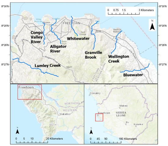
Figure 1.
Study area for framework development: Western Area Peninsula, Sierra Leone.
3. Materials and Methods
This study outlines several individual methodologies that are interconnected based on the required inputs and desired outputs. Figure 2 displays the inputs, analysis steps, and intermediate and final outputs of this study. This framework has the potential to aid in flood preparedness and mitigation and inform decisions about urban flood water management.
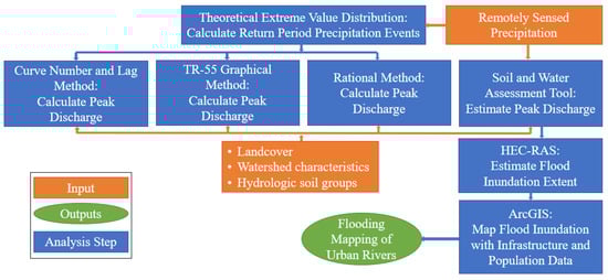
Figure 2.
Schematic of the workflow.
3.1. Precipitation Analysis
NASA’s IMERG precipitation data product was evaluated against the observed monthly data on the Western Peninsula. GPM replaced the TRMM research satellite, which collected data from 1997 to 2015. GPM had a greater frequency and broader global coverage than TRMM, among other differences. To standardize the data from TRMM and GPM, the IMERG product was developed, which converts precipitation data from TRMM, GPM, and over 20 other precipitation sensor missions into a uniform processed dataset [47]. IMERG data between 1 June 2000 and 30 November 2019 were downloaded using the NASA access tool [48].
The first step in calculating the return period storm events was to determine the largest precipitation event from each year and rank in descending order. Using the theoretical extreme value distribution approach with a Gumbel (Type I) distribution, precipitation events were calculated for return periods of 2, 5, 10, 25, 50, and 100 years in mm/day based on Equation (1), where XT is the value of the random variable associated with a given return period T; is the mean of the observations; S is the standard deviation of the observations; and KT is the frequency factor associated with return period T [49,50,51].
In addition to the daily and monthly IMERG data, observed monthly precipitation values were also assessed. The theoretical extreme value distribution approach was used by ranking the wettest month from each year (2000 to 2019) and then dividing by the number of days in each respective wettest month to be used in Equation (1) and resulted in return period precipitation events in mm/day. The monthly approach was used because during the rainy season, precipitation events are relatively constant throughout a month with rain occurring most days [52,53]. Additionally, the monthly data smooths out any inconsistencies in the daily data.
3.2. Land Use/Land Cover Scenarios
For this work, it is important to implement a LULC that is representative of the broad land cover types within the proposed Western Area Peninsula Water Fund and at a spatial scale that allows for the modification of land management practices and interventions to be assessed across scenarios. While there are many land cover products available, only three publicly available land cover and land use datasets for 2016 were considered for this study: Sentinel S2 Prototype (20 m), Copernicus, and CCI MERIS Land Cover. Both Copernicus (100 m) and CCI MERIS Land Cover (300 m) were considered too coarse a resolution, as some of the interventions under consideration were within a 30 m riparian buffer zone and to capture this, we required a 10 m–20 m resolution product.
To assess LULC accuracy of the Sentinel S2 Prototype (20 m) data for the Western Area Peninsula, two hundred random points were generated in ArcGIS and accuracy was assessed in Google Earth due to travel restrictions in place during the global COVID-19 pandemic.
After selecting a base LULC map, a business as usual (BAU) landcover was created using a normalized difference vegetation index (NDVI) analysis, which combined remote sensing and GIS to effectively display urban growth [4,54]. NDVI values were calculated from the near infrared (band 5) and red (band 4) bands of Landsat 8 imagery to identify areas on a spectrum between −1.0 and 1.0 to represent a lack of green vegetation and dense green vegetation, respectively. Many studies have shown that NDVI values can be used to determine LULC classes and can be projected forward to forecast vegetation cover [54,55,56,57,58,59,60,61]. Landsat 8 bands for the month of January in 2015 and 2020 were used to ensure cloud free imagery with similar seasonality, and Equation (2) was used to calculate the NDVI.
3.3. Peak Discharge Analysis
Using the precipitation events determined from Section 3.1, the runoff from each precipitation event was calculated based on watershed area, soil type, and LULC. The watershed areas were determined through the use of ArcHydro tools with a 1 m2 DEM. This DEM was provided by Catholic Relief Services (CRS) during the development of a Water Fund program for Freetown and the Western Area Peninsula in partnership with the Nature Conservancy (TNC). One m2 DEMs are not yet globally available but high resolution terrain data are becoming more accessible and affordable worldwide [62]. Soil texture classes were downloaded from openlandmap and reclassified into hydrologic soil groups [63,64]. LULC data were gathered from the European Space Agency (ESA) Climate Change Initiative (CCI) Land Cover Team, which produced a 20 m high resolution LULC for Africa based on Sentinel-2A observations from 2016 [65]. Three peak runoff calculations, (curve number and lag method, curve number and graphical method, and rational method) were utilized to compare the analysis to SWAT outputs. The three peak runoff calculations were performed for the Congo Valley River to determine which runoff calculation to use for all seven rivers based on comparison to the SWAT results
3.3.1. Curve Number and Lag Method
The United States Department of Agriculture (USDA) National Resources Conservation Service (NRCS) curve number (CN) method was developed empirically to estimate direct runoff from storm rainfall for small watersheds [66]. This method is frequently used where field data are unreliable or unavailable [3,4,6,34,67,68,69]. The lag method, also a product of the NRCS, is used to compute peak discharge, assuming a triangular dimensionless unit hydrograph. First, to determine the CN of the watershed, overlay features in ArcPro were used to determine the LULC (Sentinel 2016) and soil group combination for each area within the watershed, and a CN was assigned to each combination [70,71]. A composite CN was then calculated for the watershed and used to further calculate the potential maximum retention after runoff begins (S) and runoff depth (Q) [66]. The lag method was used to calculate flow length, the time of concentration, time to peak, and peak discharge, assuming a triangular hydrograph approximation [3,70,72,73]. Equation (3) represents the lag method peak discharge equation where A is the drainage area (mi2); Q is the runoff (inch) from the CN analysis; Tp is the time to peak (hours); and qp is the peak discharge (cfs).
3.3.2. Curve Number and Graphical TR-55
The graphical peak discharge method for small watersheds was developed to calculate peak runoff based on time of concentration, drainage area, rainfall distribution, 24-h rainfall, and CN for small urban watersheds [67,74]. Curve numbers were calculated as described above and then used to determine initial abstraction (Ia). Initial abstraction to precipitation ratio along with time of concentration were then used with the appropriate rainfall distribution (4I, 4IA, 4II, or 4III) from the TR-55 to determine unit peak discharge (qu). Peak discharge was calculated using Equation (3) where qp is the peak discharge (cfs); qu is the unit peak discharge (csm/in); Am is the drainage area (mi2); Q is runoff (inch); and Fp is the pond and swamp adjustment factor.
3.3.3. Rational Method
Alternatively, the rational method in Equation (4) was used to predict peak flow rates (Q), as it is designed for very small, urban watersheds based on rainfall intensity (i); watershed area (A); and a dimensionless runoff coefficient (C) [75]. Chin (2019) used the rational method for estimating peak runoff rates in urban catchments [76]. The runoff coefficient was determined based on soil and LULC, similar to the CN analysis, and the rainfall intensity assumed a constant daily rain divided by 24 h.
3.4. SWAT Precipitation and Peak Runoff Generation
ArcGIS 10.5.1 was used to parameterize the Soil and Water Assessment Tool (SWAT) version 2012 model for the Western Area Peninsula [77,78]. Hydrologic response units (HRUs) were developed with no thresholding for LULC and 20% thresholding each for soils and slope. This resulted in 11,224 HRUs distributed across the 325 sub watersheds. SWAT was run from 2000 to 2019, with a 3-year model spin-up period to reach equilibrium in the soil water content.
SWAT implements the NRCS curve number method to calculate runoff using an empirical water balance relationship:
where Q is the direct runoff (mm); P is the total rainfall (mm); and S = 1000/CN, with CN (curve number) related to soil and LULC conditions, and commonly estimated from the published tables (or tables generated by experienced hydrologists for specific locations).
Model calibration was carried out using SWAT-CUP and implementing the SUFI2 algorithm [79]. Because no stream discharge data are available for the watersheds being modeled, satellite-derived evapotranspiration (ET) from MOD16 was used for model calibration [80,81,82,83,84]). ET calibration was carried out at the subwatershed scale based on LULC type for forest, urban, cropland, and grassland.
To assess SWAT in predicting ET, a coefficient of determination (R2) was used and is a statistic commonly used to assess SWAT model performance [85,86]. R2 ranges from 0 to 1 and describes the proportion of variance in the dependent variable explained by the independent variable. Values closer to 1 indicate that the model is replicating observed data, which in this case is represented by MOD16 ET.
The theoretical extreme value distribution approach was performed on the SWAT flow outputs to determine the return period flow events for each river so that the SWAT outputs could be easily compared to the calculated peak discharges. These simulated flood events from the SWAT output return period flows were used in the HEC-RAS analysis.
3.5. HEC-RAS Setup
The Hydrologic Engineering Center’s River Analysis System (HEC-RAS) was used to model seven urban rivers in Freetown: Alligator River, Congo Valley River, Granville Brook, Wellington Creek, Lumley Creek, Whitewater, and Bluewater. The 1 m2 DEM provided by CRS was imported into RAS-Mapper, the projection was set to WGS 1984 UTM Zone 28N, and a terrain file was created to encompass the urban rivers [87]. In RAS-Mapper, the 1 m2 DEM was used to draw the river, bank, and flow path lines based on the elevation differences observed from the DEM and cross sections were drawn perpendicularly to flow lines at approximately 25 m spacing [87]. Manning’s n values were assigned as 0.040 for the channel within the banks to represent developed, open space, and as 0.0678 for the overbanks to represent the medium to high intensity developed areas [88]. Due to data limitations, a steady flow analysis was used for the 1D model. The peak flow for each return period from the SWAT outputs was added to the steady flow editor at the most upstream cross section and an assumption of normal depth was used for the downstream boundary condition by approximating the energy slope as the slope of the channel bottom from the DEM. The steady flow analysis was run as subcritical. Inundation boundary layers were created for all return period events from the 1D steady flow analysis in RAS-Mapper. A 2D mesh HEC-RAS analysis with an unsteady flow file was also attempted because a 2D modeling approach is often suggested for complex river systems, however, data limitations and the steep slope gradients on the peninsula lead to unreliable results [68]. Most successful 2D models are carried out on gauged watersheds that have a plethora of hydrologic and hydraulic information to ensure accurate estimation of flood extents, but under limited data circumstances, 2D models are much more difficult to use to accurately represent flood extents, especially in urban areas [68].
3.6. Geospatial Analysis
Geographic information system (GIS) software ArcGIS Pro 2.6.1 was used in this analysis for its ability to manage and analyze the hydrological parameters in urban areas [4,89]. The inundation boundary layers created in RAS-Mapper from the previous section were imported to ArcPro. The area of each inundation polygon was recorded in square kilometers. A building shapefile and a 30 × 30 m population raster from 2015 provided by CRS were imported to ArcPro. ModelBuilder was used to iterate the clipping of the building shapefile for each inundation boundary for the various rivers, return periods, and LULC scenarios. The number of buildings present in each clip was recorded and represents the number of buildings affected by a particular flood inundation boundary. ModelBuilder was also used to iterate the zonal statistics as a table tool for each inundation boundary to determine the sum of the population raster affected by each boundary. This sum represents the total number of people affected by the flood boundary.
4. Results
4.1. Precipitation Analysis
Over the 20-year time frame, from 2000 to 2019, the IMERG data underestimated total monthly precipitation in comparison to the observed data where the observed and IMERG total precipitations were 59,115 mm and 57,623 mm, respectively, which equates to approximately 100 mm per year difference.
Return period precipitation results of the theoretical extreme value distribution approach performed on the IMERG and observed data are presented in Table 1. With the lack of daily observed data, it is difficult to determine whether the daily IMERG values represent the precipitation in Freetown properly, however, the monthly comparisons provide some insight. As can be seen in Table 1, the return period events from the observed monthly values were consistently higher than the IMERG return events, leading to the assumption that IMERG likely underestimates daily precipitation [90]. Unfortunately, with the lack of daily observed data and the gaps in the monthly observed data over the period of interest (2000 to 2019), the observed data could not be used in the SWAT analysis, and instead, the use of remotely sensed precipitation data was required. The IMERG dataset includes data from TRMM and over 20 other precipitation sensor missions [47]. Additionally, the IMERG spatial resolution (0.1°) allowed coverage over the peninsula to account for the changes in precipitation due to changing topography and covered the period of interest (2000–2019).

Table 1.
Calculated return period precipitation events (mm/day) from various datasets.
4.2. Land Use/Land Cover Scenarios
Results of the Sentinel S2 Prototype land cover assessment are included in Table S1 and indicate an overall map accuracy of 78.5%. We found that most confusion occurred around LULC class edges and in classes with little areal coverage. In terms of LULC edges, this may be explained by the rapid land cover change—particularly expanding agriculture–occurring and not being able to ensure anniversary date images across Google Earth and Sentinel S2 products. Some land use classes such as shrubland and wetland comprise only 1% and 5% of the area, respectively, and would require field training data and validation.
Using the Sentinel-2A LULC as a baseline, the 2015 NDVI values were reclassified to align with the Sentinel-2A LULC. Figure 3C displays the Sentinel-2A LULC map and 3A displays the LULC map created from the 2015 NDVI reclassifications.
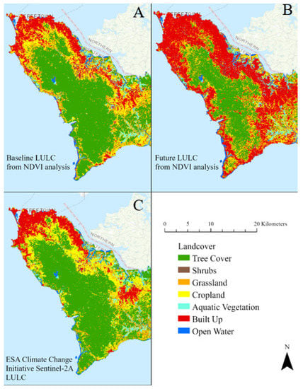
Figure 3.
Development of future LULC map. (A) Baseline LULC map developed from reclassification of NDVI values. (B) Future LULC map developed from projection and reclassification of NDVI values. (C) Template baseline LULC map from ESA Climate Change Initiative Sentinel-2A.
The NDVI values and LULC groups generated from this alignment with Sentinel-2A are presented in Table 2. With the use of Raster Calculator in ArcPro, the percent change in NDVI values from the years 2015 to 2020 was projected forward to calculate NDVI values for the year 2050. The 2050 NDVI values were then reclassified to fit the LULC categories based on the NDVI value groups presented below. The LULCs of aquatic vegetation, shrub, and water were assumed to be constant throughout the years and did not fit a NDVI value group. Figure 3B displays the 2050 NDVI reclassification map. Additionally, Table S2 in the Supplementary Materials indicates the accuracy assessment for the NDVI image, and Table S3 in the Supplementary Materials displays the percentages of each land cover class for the Sentinel-2A LULC map and the 2015 and 2050 NDVI LULC maps. The NDVI map has an overall 70.5% accuracy.
Table 2.
LULCs for each NDVI value group.
Peak discharge calculations were performed for the baseline LULC from the ESA CCI Sentinel-2A and compared to the baseline analysis performed in SWAT. Additionally, SWAT analyses were performed for a future 2050 BAU scenario, which assumes that management of the peninsula’s land continues as is without sustainable conversation solutions or slowing the rate of urbanization. The SWAT return period flows from the baseline and BAU LULC scenarios were used as inputs for the following HEC-RAS analysis.
4.3. Peak Runoff Analysis
Using the IMERG generated return period precipitation events, three equations were used to calculate the peak discharge and compared to SWAT outputs. The CNs calculated for the baseline LULC scenario used for two of the peak discharge calculations represents the imperviousness of the watersheds. Over all seven urban rivers, the CN ranged from a low of 79 in the Granville Brook watershed to a high of 88 in the Alligator River and Congo Valley River watersheds. These high CNs represent the high level of urbanization in the Freetown area, which has resulted in highly impervious watersheds [70].
Using the CNs, the lag method and graphical TR-55 methods were utilized to calculate peak discharge. Additionally, the rational equation was used, which incorporates a runoff coefficient to represent LULC and soil type similar to the curve number approach. The three calculations were performed for the Congo Valley River to determine the most appropriate runoff calculation in comparison to the SWAT flow outputs. The calculated runoff values are presented and compared to the SWAT outputs in Table 3. The rational and graphical TR-55 methods drastically underestimate the flows in comparison to the SWAT outputs while the lag method compared much better to the SWAT outputs.
Table 3.
Comparison of flow calculation methods for the Congo Valley River baseline LULC.
The calculations for Congo Valley River show that the lag method compares the best to SWAT outputs, therefore, the lag method was used to calculate peak discharge for all seven rivers. Table 4 displays the peak runoff comparison between the lag method calculations and SWAT outputs for all urban rivers and all return period events. The results did not show any constant trends between the lag method and the SWAT outputs for the return period events over all rivers. For example, for the Alligator River, the lag method calculation results were slightly higher than the SWAT outputs for all of the return period events while for the other rivers, the lag method calculation results were lower than the SWAT outputs. Additionally, the difference between the lag method and SWAT outputs varied for each river and each return period. For example, the lag method calculates peak discharges about 10 m3/s less than the SWAT outputs for all return periods for Lumley Creek, while the difference was less than 2 m3/s for all return periods for Whitewater. Overall, there were some discrepancies between the two approaches, however, in general, the lag method calculations compared well to SWAT and therefore could be used for the HEC-RAS analysis, however, for consistency purposes throughout the research team, this paper utilized the SWAT outputs for the HEC-RAS analysis.
Table 4.
Comparison of peak discharges (m3/s) for baseline LULC.
R2 was used as the objective function for assessing SWAT model performance. R2 values for forest were the lowest when assessing across all months, ranging from 0.2 to 0.25. When excluding dry season months, R2 values increased to 0.7–0.75. R2 for built up areas ranged from 0.7 to 0.8, and over cropland ranged from 0.4 to 0.7 and on grasslands from 0.75 to 0.8.
4.4. Inundation Areas and Affected Infrastructure and Population
Using the SWAT flow outputs displayed in Table 4 as well as the outputs for the BAU LULC scenario, HEC-RAS models were performed for all seven urban rivers and inundation boundaries were created for each return period flow. Figure 4 displays the number of people affected by each return period flow and the inundation areas. Additionally, tables in the Supplementary Material display the area, population, and number of buildings affected in each watershed.
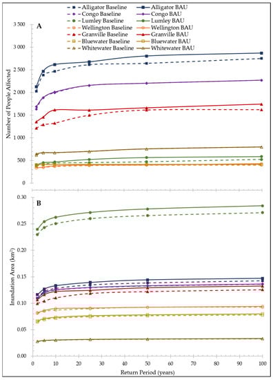
Figure 4.
(A) Number of people affected by each return period storm for all seven urban rivers. (B) Inundation area from each return period storm for all seven urban rivers.
The inundation areas and number of people affected were higher for the BAU than the baseline LULC, as expected. The BAU scenario resulted in much more built up LULC and much less forested and cropland areas than the baseline. This increase in built up area increases imperviousness and thus runoff, which becomes river flow. For just a two year storm, the inundation boundaries of the urban rivers affected a total of 6584 people for the baseline LULC and increased to 6956 people from the BAU LULC. It is also evident that larger return period storms cause more flood impacts. For example, for the Congo Valley River baseline LULC scenario, the two year storm affected 1630 people while the 100 year affected 2270 people. This points out that larger storm events cause more flood impacts and need to be mitigated in the future, especially as climate change causes more frequent and larger precipitation events [8,9,91]. Additionally, the largest increases in affected population from the baseline to BAU scenario typically occur for smaller return period storms. For the Congo Valley River example, the BAU LULC causes flooding to affect a population of 1686 people for the two year storm and a population of 2270 for the 100 year storm. The difference in LULC from the baseline to BAU caused an increase in people affected by a two year storm, but no additional people to be affected from a 100 year storm. It is evident that the continued urbanization of Freetown will lead to further encroachment on the waterways, which will increase the number of people affected by flood events.
4.5. Inundation Boundary Validation
Due to the lack of precipitation and flow data available to calibrate the SWAT and HEC-RAS models, the inundation boundaries were compared to various sources of historic floods and global open source flood modeling results to determine their validity. University College London, in collaboration with the Sierra Leone Urban Research Center, documented, mapped, and recorded interviews of historic urban risks including but not limited to fire outbreaks, rock falls, waste dumping, and floods and made these data available for viewing on their website, ReMapRisk Freetown [92]. A maximum water extent raster representing all the locations ever detected as water between 1984 and 2019 was also compared [93]. The maximum water extent raster was developed using Landsat satellite imagery at 30 m resolution and was made available as part of the Joint Research Center’s Global Surface Water Dataset [93]. The resolution does not pick up the narrow urban rivers in the upstream extents, but rather shows the flooding near the coast. Coastal flooding reflects coastal areas of near sea level topography. These areas are flooded due to coastal storm surge events, while the focus of this study was to estimate fluvial flooding. Figure 5 displays the historic flood points, maximum water extent raster, and the HEC-RAS modeled inundation boundaries for the 100 year storm event for the BAU LULC scenario, which would be considered the worst case scenario in terms of simulated flood extents and people and infrastructure affected. The two through 50 year return period storm inundation areas were also assessed. Results showed that the incised river upstream and flat landscape downstream had relatively small changes to flood extent for varying return period storms. The 100 year storm event with the BAU LULC resulted in the largest inundation areas and most flood impacts.
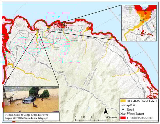
Figure 5.
HEC-RAS modeled flood extents compared to historic flood event points and maximum water extent.
It should be noted that the maximum water extent raster represents coastal flooding as it is unable to capture streams and rivers of the scale present in this study, and therefore, does not represent the upstream extent of urban riverine flooding. In comparison to this raster, the HEC-RAS modeled flood inundations closely aligned, but slightly underestimated flood extents near the coast. This discrepancy is likely due to tidal impacts and storm surges that HEC-RAS does not consider. Similarly, while the historic flood event points align well with the model outputs, the points were predominately lower downstream, into the coastal zone, and did not include the full extent of the watershed or all of the urban streams modeled. In the upper right inset image of Figure 5, it is evident that the HEC-RAS flood extents are capturing historic flood events in the Alligator River area. The bottom left zoomed image displays a large flood event from August 2017 in the Congo-Cross area [45]. By comparing the water level to the height of the people in the image, it can be estimated that the water was slightly greater than 1.0 m in depth (chest high). In comparison, the HEC-RAS modeled depth was about 1.0 m for the downstream extent of the Congo Valley River. Due to the limitations of observational data, these comparisons to the maximum water extent raster, historic flood points, and flood image were the best comparison available. Despite the slight discrepancies between the flood estimates collected online and the HEC-RAS flood extents, the visual comparisons showed that the HEC-RAS inundations are likely to be representative of the flood events occurring on the Western Area Peninsula.
5. Discussion
5.1. Precipitation Analysis
Two precipitation datasets were assessed for use in calculating return period storms and ultimately peak runoff in Freetown, Sierra Leone: IMERG daily data and observed monthly. When IMERG precipitation data were analyzed against limited monthly observed precipitation in Freetown, we determined that this was an acceptable data choice. The IMERG data were particularly advantageous in this study because of its ability to capture spatial variation and the statistics for the monthly aggregation of IMERG data were consistent with the monthly observed data. The raw data and the calculated return period events showed that the IMERG data underestimated precipitation in comparison with the overserved values, however, in general, the IMERG return period events closely track the return period events from the observed data.
5.2. Land Use/Land Cover Scenarios
The 2015 NDVI reclassification map is not an exact replication of the Sentinel-2A map. Specifically, the 2015 NDVI reclassification map slightly overpredicted built up LULC in areas that are presented as cropland from the Sentinel-2A LULC map around the forest border. Additionally, the 2015 NDVI reclassification map showed some cropland and grassland where the Sentinel-2A LULC map only showed built up LULC. Overall, the 2015 NDVI reclassification map displayed LULC groups similarly to those displayed in the Sentinel-2A LULC map. Due to the slight differences between the 2015 NDVI reclassification map and the Sentinel-2A LULC map, it is likely that the 2050 LULC also slightly overestimated built up area and underestimated cropland, especially around the forest boundary, however, in the absence of other LULC projections, this was used to map the BAU scenarios in SWAT.
5.3. Runoff Calculations
The curve numbers of the seven urban watersheds in Freetown are high, which represents increased runoff potential. These high CNs are expected due to the large amount of impervious area from built up LULC, and is reflected in the urban hydrograph [94,95,96]. Urban CN values are always relatively high due to the associated impervious surface [74,97,98]. In this region, where soil hydrologic features are fairly consistent, relatively similar CN values are expected. Ultimately, these high CNs lead to larger amounts of precipitation contributing to surface runoff and making its way to rivers instead of infiltrating the ground, resulting in a more dramatic flood pulse [3,4]. The CN method has a several limitations including the possible underestimation of runoff depth due to compositing CNs throughout a watershed, but the method is long-established and well-respected and will continue to be used because it is computationally simple and appears to give reasonable results [3,67,69,98,99].
In addition to runoff depth from the CN analysis, peak discharge was also calculated through the lag, rational, and graphical methods. These methods are simplifications of reality, which in certain cases are fair representations of the surface water hydrology when more complex models are not feasible [74,100]. The rational and graphical methods severely underestimate peak discharge for all return period events under the baseline LULC scenario for the Congo Valley River in comparison to the SWAT flow outputs. While some discrepancy was anticipated due to assumptions around the input parameters, the rational method was roughly 10% of the SWAT outputs (Table 3). The rational method does not accurately represent the peak discharge in the urban rivers because it was developed for smaller watersheds than those on the Western Area Peninsula [75,76]. Similarly, the graphical TR-55 method does not apply well to the Freetown watersheds because the initial abstraction to precipitation ratio is outside the range, therefore, the limiting value on the graphs was used [75]. Generally, the lag method compared relatively well to the SWAT output, showing that the lag method coupled with remotely sensed data can be used to estimate peak discharge in ungauged watersheds and further used to map flood extents in HEC-RAS, however, in this analysis, the SWAT flow outputs were used in HEC-RAS.
5.4. Inundation Estimations
The peak discharge for the baseline and BAU LULC scenarios were used in HEC-RAS to determine flood impacts for each river. As expected, the BAU LULC scenario resulted in more flood impacts than the baseline scenario because of the increase in impervious area, and larger return period storms resulted in more flood impacts due to higher peak discharges. These results are consistent with other urban fluvial flooding studies, which have shown a link between urban LULC and flood frequency [101,102,103]. One unexpected finding of this analysis is that throughout the seven urban rivers, most of the largest differences between the baseline and BAU scenarios, in terms of inundation area and people affected, occurred for smaller, more frequent storms than the larger return periods. It is widely known that a 100 year storm will result in flooding in most areas, but this analysis shows that smaller, more frequent storms may be just as detrimental to an area, especially as urbanization increases. Additionally, at a certain threshold, the floodwaters can no longer expand horizontally into and beyond the floodplain due to topographic limitations. Once this threshold is met, increased storm events will result in the same population affected, but the water will be deeper and move more quickly, which significantly increases the potential harm to that population [104].
Due to a lack of field data, the research team could not ground truth or calibrate the SWAT and HEC-RAS models. Landsat satellite imagery could not be used to pinpoint flood extents because of vast cloud cover over the peninsula during and in the days following large precipitation events. Furthermore, in many urban areas, the resolution of the imagery is too coarse to capture the narrow urban rivers tightly bound by development along the banks and in the floodplain [105,106,107]. At this time, there is no available site specific reference data to definitively determine the accuracy of the results, but to ensure that the models are producing realistic results, they were compared to previously published resources such as images of flood events, known historic areas of flooding, and global open source modeled flood extents. Table S4 in the Supplementary Materials summarizes all data sources used. These comparisons show that the HEC-RAS modeled flood extents and depths are realistic. During the period of this study, the COVID-19 pandemic made it impossible for this research team to travel to Freetown to perform a site visit and collect data for calibration and ground truth model results. Although a site visit would have helped to inform the analysis, this study shows the value in leveraging remotely sensed data when field data are limited.
Although this analysis was performed for a case study in Freetown, Sierra Leone, the datasets and methods are available to be used in other areas around the world where field data are lacking. The LULC, soil, and precipitation datasets are all globally available for use around the world, and open source population and building datasets can be downloaded for other areas, although in this case, they were provided by Catholic Relief Services. The 1 m2 digital elevation model (DEM) dataset for the Freetown area was also provided by Catholic Relief Services. The 1 m2 DEM was instrumental in creating the HEC-RAS models and determining watershed characteristics for the peak discharge calculations. While 1 m2 DEMs are not globally available, as the data revolution progresses, the availability of high resolution terrain data is becoming increasing obtainable, which has the potential to be very beneficial for fine resolution flood modeling for flood risk areas [62]., Rapid advancements in Lidar data collection are allowing for this type of data to be increasingly accessible. For example, the development of photogrammetry techniques in unmanned aerial vehicles can be a low cost alternative to LiDAR because they produce DEMs comparable to those from LiDAR for fluvial assessment applications and urban environments [108].
Additionally, more remotely sensed datasets for calibration and verification purposes are becoming available, but are not currently feasible for validating this model. Cloud cover limits the application of satellite imagery, while urban backscatter poses challenges for the use of synthetic-aperture radar (SAR) data. NASA’s Surface Water Ocean Topography (SWOT) mission, which is set to launch in 2022, aims to provide discharge estimates for rivers with widths greater than 100 m, allowing for hydrologic and hydraulic model calibration in ungauged areas [109].
6. Conclusions
In Freetown, Sierra Leone, urban flooding has been exacerbated by LULC changes from vegetated areas to urban development due to increasing population. This development has occurred near riverbanks and within the floodplain, leading to dangerous conditions for infrastructure and the human population that has settled there. Hydrologic and hydraulic modeling was performed using remotely sensed data to map the flood extents, which can be used to warn the population that may be at risk, for disaster recovery planning, or for disaster recovery management. To determine the impacts of future flood events, a future 2050 LULC scenario was created through a normalized difference vegetation index (NDVI) analysis with the use of Landsat Imagery and Sentinel-2A LULC classifications and compared to the 2015 baseline scenario. In addition to LULC, future precipitation events were calculated to represent return period storms. Due to a lack of reliable, long term precipitation data, two remotely sensed precipitation datasets, Tropical Rainfall Measuring Mission (TRMM) and Integrated Multi-satellitE Retrievals for GPM (IMERG) where GPM is the Global Precipitation Mission, were used with the theoretical extreme value distribution approach to calculate return period precipitation for the 2, 5, 10, 25, 50, and 100 year events. The IMERG dataset was used as an input for peak discharge calculations and a separate Soil and Water Assessment Tool (SWAT) analysis. The curve number (CN) and lag method, CN and graphical TR-55, and rational equation methods were used to calculate peak discharge for an urban river and compared to the flow outputs from the SWAT analysis. The CN and lag method peak discharges compared well to the SWAT flow outputs, showing that these calculations with remotely sensed precipitation data can represent the discharge in urban rivers. To determine the simulated flood extents of the rivers, seven 1D HEC-RAS models were created. The inundation boundaries from HEC-RAS were used to evaluate the population and buildings impacted. In the absence of field data for precipitation and river flows, the modeled flood extents were compared to historic flood points, images of flood events, and a global maximum surface water extent from the Joint Research Center’s Global Surface Water Dataset.
This study presents a framework for calculating peak discharge and mapping urban floods and demonstrates that remotely sensed input data can be used to correctly identify inundated areas of return period storms. The framework for calculating peak discharges and mapping flood extents presented in this paper can be used to estimate discharge in other ungauged urban watersheds around the world. Many watersheds around the world are data scarce, particularly in resource stressed locations such as least developed countries (LDC). Insufficient data make hydrologic and hydraulic modeling difficult, impeding flood modeling critical for proper warning systems, evacuation plans, and disaster management. Here, we present an approach for smaller urban streams that is relatively simple and obtainable for general engineering analysis, which utilizes mostly globally open source data. Although the high-resolution elevation data are not yet globally available, advancements in technology will lead to more accessible data in the coming years. Findings from this study showed, even lacking robust methods and model calibration data, remotely sensed precipitation can be used to estimate runoff from empirical calculations and software such as SWAT. Using these runoff results, a 1D HEC-RAS analysis can properly identify flood inundation boundaries. Ultimately, this framework provides an obtainable means for informing decisions about urban stormwater management and design to reduce the losses associated with urban floods.
Supplementary Materials
The following are available online at https://www.mdpi.com/article/10.3390/rs13193806/s1, Table S1: Accuracy assessment of 2016 Sentinel S2 Protype LULC product against GoogleEarth imagery; Table S2: Accuracy assessment of 2015 NDVI LULC product against GoogleEarth imagery; Table S3: LULC categories of the Western Area Peninsula; Table S4: Data Sources; Table S5: Alligator River; Table S6: Congo Valley River; Table S7: Lumley Creek; Table S8: Wellington Creek; Table S9: Granville Brook; Table S10: Bluewater; Table S11: Whitewater; Table S12: All Urban Rivers.
Author Contributions
Conceptualization, A.C. and V.S.; Methodology, A.C.; Software, A.C., T.B. and R.S.; Validation, A.C., T.B. and R.S.; Formal analysis, A.C.; Investigation, A.C.; Resources, V.S., T.B. and R.S.; Data curation, A.C., V.S., T.B. and R.S.; Writing—original draft preparation, A.C.; Writing—review and editing, V.S., T.B. and R.S.; Visualization, A.C.; Supervision, V.S.; Project administration, V.S.; Funding acquisition, V.S. All authors have read and agreed to the published version of the manuscript.
Funding
This research was funded by Catholic Relief Services for the development of a Water Fund for the Peninsula in partnership with The Nature Conservancy and the Villanova University College of Engineering Department of Civil and Environmental Engineering as well as contributions from an anonymous donor.
Institutional Review Board Statement
Not applicable.
Informed Consent Statement
Not applicable.
Data Availability Statement
Generally, the data used in this study is available in public repositories (sources can be found in the references). The exception is the 1 m2 DEM, which was obtained by Catholic Relief Services and made available to the authors with the permission of Catholic Relief Services.
Acknowledgments
This paper was completed with support from Catholic Relief Services for the development of a Water Fund for the Peninsula in partnership with The Nature Conservancy (TNC) and the Villanova University College of Engineering Department of Civil and Environmental Engineering. Technical support was received from TNC and the faculty, staff, and peers of the Villanova Center for Resilient Water Systems (VCRWS).
Conflicts of Interest
The authors declare no conflict of interest.
References
- United Nations; Department of Economic and Social Affairs; Population Division. World Population Prospects 2019: Highlights; UN: New York, NY, USA, 2019; ISBN 978-92-1-148316-1. [Google Scholar]
- Ahiablame, L.M.; Engel, B.A.; Chaubey, I. Effectiveness of Low Impact Development Practices: Literature Review and Suggestions for Future Research. Water Air Soil Pollut. 2012, 223, 4253–4273. [Google Scholar] [CrossRef]
- Blair, A.; Sanger, D.; White, D.; Holland, A.F.; Vandiver, L.; Bowker, C.; White, S. Quantifying and Simulating Stormwater Runoff in Watersheds: STORMWATER RUNOFF IN WATERSHEDS. Hydrol. Process. 2014, 28, 559–569. [Google Scholar] [CrossRef]
- Weng, Q. Modeling Urban Growth Effects on Surface Runoff with the Integration of Remote Sensing and GIS. Environ. Manag. 2001, 28, 737–748. [Google Scholar] [CrossRef] [PubMed]
- Sheng, J.; Wilson, J.P. Watershed Urbanization and Changing Flood Behavior across the Los Angeles Metropolitan Region. Nat. Hazards 2009, 48, 41–57. [Google Scholar] [CrossRef]
- Suriya, S.; Mudgal, B.V. Impact of Urbanization on Flooding: The Thirusoolam Sub Watershed—A Case Study. J. Hydrol. 2012, 412–413, 210–219. [Google Scholar] [CrossRef]
- Rogger, M.; Agnoletti, M.; Alaoui, A.; Bathurst, J.C.; Bodner, G.; Borga, M.; Chaplot, V.; Gallart, F.; Glatzel, G.; Hall, J.; et al. Land Use Change Impacts on Floods at the Catchment Scale: Challenges and Opportunities for Future Research: Land Use Change Impacts on Floods. Water Resour. Res. 2017, 53, 5209–5219. [Google Scholar] [CrossRef] [PubMed]
- Saldarriaga, J.; Salcedo, C.; Solarte, L.; Pulgarín, L.; Rivera, M.L.; Camacho, M.; Iglesias-Rey, P.L.; Martínez-Solano, F.J.; Cunha, M. Reducing Flood Risk in Changing Environments: Optimal Location and Sizing of Stormwater Tanks Considering Climate Change. Water 2020, 12, 2491. [Google Scholar] [CrossRef]
- Li, L.; Jiang, C.; Murtugudde, R.; Liang, X.-Z.; Sapkota, A. Global Population Exposed to Extreme Events in the 150 Most Populated Cities of the World: Implications for Public Health. Int. J. Environ. Res. Public Health 2021, 18, 1293. [Google Scholar] [CrossRef]
- Eleutério, J.; Hattemer, C.; Rozan, A. A Systemic Method for Evaluating the Potential Impacts of Floods on Network Infrastructures. Nat. Hazards Earth Syst. Sci. 2013, 13, 983–998. [Google Scholar] [CrossRef]
- United Nations; Department of Economic and Social Affairs. World Social Report 2020: Chapter 3: Climate Change Exacerbating Poverty and Inequality; UN: New York, NY, USA, 2020; ISBN 978-92-1-130392-6. [Google Scholar]
- Mahmoud, S.H.; Gan, T.Y. Urbanization and Climate Change Implications in Flood Risk Management: Developing an Efficient Decision Support System for Flood Susceptibility Mapping. Sci. Total Environ. 2018, 636, 152–167. [Google Scholar] [CrossRef]
- Proag, V. The Concept of Vulnerability and Resilience. Procedia Econ. Financ. 2014, 18, 369–376. [Google Scholar] [CrossRef]
- Mohamed, S.A.; El-Raey, M.E. Vulnerability Assessment for Flash Floods Using GIS Spatial Modeling and Remotely Sensed Data in El-Arish City, North Sinai, Egypt. Nat. Hazards 2020, 102, 707–728. [Google Scholar] [CrossRef]
- National Research Council. Elevation Data for Floodplain Mapping; National Academies Press: Washington, DC, USA, 2007; p. 11829. ISBN 978-0-309-10409-8. [Google Scholar]
- Apel, H.; Aronica, G.T.; Kreibich, H.; Thieken, A.H. Flood Risk Analyses—How Detailed Do We Need to Be? Nat. Hazards 2009, 49, 79–98. [Google Scholar] [CrossRef]
- Glas, H.; Deruyter, G.; De Maeyer, P.; Mandal, A.; James-Williamson, S. Analyzing the Sensitivity of a Flood Risk Assessment Model towards Its Input Data. Nat. Hazards Earth Syst. Sci. 2016, 16, 2529–2542. [Google Scholar] [CrossRef]
- Bates, P.D.; Wilson, M.D.; Horritt, M.S.; Mason, D.C.; Holden, N.; Currie, A. Reach scale floodplain inundation dynamics observed using airborne synthetic aperture radar imagery: Data analysis and modelling. J. Hydrol. 2006, 328, 306–318. [Google Scholar] [CrossRef]
- Aggett, G.R.; Wilson, J.P. Creating and Coupling a High-Resolution DTM with a 1-D Hydraulic Model in a GIS for Scenario-Based Assessment of Avulsion Hazard in a Gravel-Bed River. Geomorphology 2009, 113, 21–34. [Google Scholar] [CrossRef]
- Masser, I. Managing Our Urban Future: The Role of Remote Sensing and Geographic Information Systems. Habitat Int. 2001, 25, 503–512. [Google Scholar] [CrossRef]
- Boongaling, C.G.K.; Faustino-Eslava, D.V.; Lansigan, F.P. Modeling Land Use Change Impacts on Hydrology and the Use of Landscape Metrics as Tools for Watershed Management: The Case of an Ungauged Catchment in the Philippines. Land Use Policy 2018, 72, 116–128. [Google Scholar] [CrossRef]
- Rafiei Sardooi, E.; Azareh, A.; Choubin, B.; Barkhori, S.; Singh, V.P.; Shamshirband, S. Applying the Remotely Sensed Data to Identify Homogeneous Regions of Watersheds Using a Pixel-Based Classification Approach. Appl. Geogr. 2019, 111, 102071. [Google Scholar] [CrossRef]
- Radwan, F.; Alazba, A.A.; Mossad, A. Estimating Potential Direct Runoff for Ungauged Urban Watersheds Based on RST and GIS. Arab. J. Geosci. 2018, 11, 748. [Google Scholar] [CrossRef]
- Brivio, P.A.; Colombo, R.; Maggi, M.; Tomasoni, R. Integration of Remote Sensing Data and GIS for Accurate Mapping of Flooded Areas. Int. J. Remote Sens. 2002, 23, 429–441. [Google Scholar] [CrossRef]
- Klemas, V. Remote Sensing of Floods and Flood-Prone Areas: An Overview. J. Coast. Res. 2015, 314, 1005–1013. [Google Scholar] [CrossRef]
- Wang, Y. Advances in Remote Sensing of Flooding. Water 2015, 7, 6404–6410. [Google Scholar] [CrossRef]
- Hong, Y.; Adler, R.F.; Hossain, F.; Curtis, S.; Huffman, G.J. A First Approach to Global Runoff Simulation Using Satellite Rainfall Estimation: TECHNICAL NOTE. Water Resour. Res. 2007, 43. [Google Scholar] [CrossRef]
- Li, L.; Xu, T.; Chen, Y. Improved Urban Flooding Mapping from Remote Sensing Images Using Generalized Regression Neural Network-Based Super-Resolution Algorithm. Remote Sens. 2016, 8, 625. [Google Scholar] [CrossRef]
- Psomiadis, E.; Diakakis, M.; Soulis, K.X. Combining SAR and Optical Earth Observation with Hydraulic Simulation for Flood Mapping and Impact Assessment. Remote Sens. 2020, 12, 3980. [Google Scholar] [CrossRef]
- Khan, S.I.; Hong, Y.; Wang, J.; Yilmaz, K.K.; Gourley, J.J.; Adler, R.F.; Brakenridge, G.R.; Policelli, F.; Habib, S.; Irwin, D. Satellite Remote Sensing and Hydrologic Modeling for Flood Inundation Mapping in Lake Victoria Basin: Implications for Hydrologic Prediction in Ungauged Basins. IEEE Trans. Geosci. Remote Sens. 2011, 49, 85–95. [Google Scholar] [CrossRef]
- Wilson, J.P.; Gallant, J.C. (Eds.) Terrain Analysis: Principles and Applications; Wiley: New York, NY, USA, 2000; ISBN 978-0-471-32188-0. [Google Scholar]
- Sharif, H.O.; Al-Juaidi, F.H.; Al-Othman, A.; Al-Dousary, I.; Fadda, E.; Jamal-Uddeen, S.; Elhassan, A. Flood Hazards in an Urbanizing Watershed in Riyadh, Saudi Arabia. Geomat. Nat. Hazards Risk 2016, 7, 702–720. [Google Scholar] [CrossRef]
- Elaji, A.; Ji, W. Urban Runoff Simulation: How Do Land Use/Cover Change Patterning and Geospatial Data Quality Impact Model Outcome? Water 2020, 12, 2715. [Google Scholar] [CrossRef]
- Meresa, H. Modelling of River Flow in Ungauged Catchment Using Remote Sensing Data: Application of the Empirical (SCS-CN), Artificial Neural Network (ANN) and Hydrological Model (HEC-HMS). Model. Earth Syst. Environ. 2018, 5, 257–273. [Google Scholar] [CrossRef]
- Abdrabo, K.I.; Kantoush, S.A.; Saber, M.; Sumi, T.; Habiba, O.M.; Elleithy, D.; Elboshy, B. Integrated Methodology for Urban Flood Risk Mapping at the Microscale in Ungauged Regions: A Case Study of Hurghada, Egypt. Remote Sens. 2020, 12, 3548. [Google Scholar] [CrossRef]
- Belayneh, A.; Sintayehu, G.; Gedam, K.; Muluken, T. Evaluation of Satellite Precipitation Products Using HEC-HMS Model. Model. Earth Syst. Environ. 2020, 6, 2015–2032. [Google Scholar] [CrossRef]
- Pang, J.; Zhang, H.; Xu, Q.; Wang, Y.; Wang, Y.; Zhang, O.; Hao, J. Hydrological Evaluation of Open-Access Precipitation Data Using SWAT at Multiple Temporal and Spatial Scales. Hydrol. Earth Syst. Sci. 2020, 24, 3603–3626. [Google Scholar] [CrossRef]
- Liu, Z.; Ostrenga, D.; Teng, W.; Kempler, S. Tropical Rainfall Measuring Mission (TRMM) Precipitation Data and Services for Research and Applications. Bull. Am. Meteorol. Soc. 2012, 93, 1317–1325. [Google Scholar] [CrossRef]
- Dezfuli, A.K.; Ichoku, C.M.; Huffman, G.J.; Mohr, K.I.; Selker, J.S.; Van De Giesen, N.; Hochreutener, R.; Annor, F.O. Validation of IMERG precipitation in Africa. J. Hydrometeorol. 2017, 18, 2817–2825. [Google Scholar] [CrossRef] [PubMed]
- Brocca, L.; Massari, C.; Pellarin, T.; Filippucci, P.; Ciabatta, L.; Camici, S.; Kerr, Y.H.; Fernández-Prieto, D. River flow prediction in data scarce regions: Soil moisture integrated satellite rainfall products outperform rain gauge observations in West Africa. Sci. Rep. 2020, 10, 12517. [Google Scholar] [CrossRef]
- Emberson, R.; Kirschbaum, D.; Stanley, T. New global characterisation of landslide exposure. Nat. Hazards Earth Syst. Sci. 2020, 20, 3413–3424. [Google Scholar] [CrossRef]
- Cui, Y.; Cheng, D.; Choi, C.E.; Jin, W.; Lei, Y.; Kargel, J.S. The cost of rapid and haphazard urbanization: Lessons learned from the Freetown landslide disaster. Landslides 2019, 16, 1167–1176. [Google Scholar] [CrossRef]
- Baker, T.; Srinivasan, R.; Apse, C. SWAT (Soil and Water Assessment Tool) Simulation of Forest Interventions on Stream Discharge and Sediment Yield in the Western Area Peninsula, Sierra Leone; The Nature Conservancy: Arlington, TX, USA, 2020. [Google Scholar]
- Statistics Sierra Leone. 2015 Population and Housing Census Summary of Final Results; Statistics Sierra Leone: Freetown, Sierra Leone, 2016. [Google Scholar]
- World Bank Group. Sierra Leone Multi-City Hazard Review and Risk Assessment (Vol. 2): Freetown City Hazard and Risk Assessment: Final Report (English); World Bank Group: Washington, DC, USA, 2018; Available online: http://documents.worldbank.org/curated/en/151281549319565369/Freetown-City-Hazard-and-Risk-Assessment-Final-Report (accessed on 9 September 2021).
- Gbanie, S.; Griffin, A.; Thornton, A. Impacts on the Urban Environment: Land Cover Change Trajectories and Landscape Fragmentation in Post-War Western Area, Sierra Leone. Remote Sens. 2018, 10, 129. [Google Scholar] [CrossRef]
- Blumenfeld, J. From TRMM to GPM: The Evolution of NASA Precipitation Data|Earthdata. Available online: https://earthdata.nasa.gov/learn/articles/tools-and-technology-articles/trmm-to-gpm (accessed on 18 January 2021).
- Mohammed, I.N. NASAaccess-Downloading and Reformatting Tool for NASA Earth Observation Data Products [Software]; National Aeronautics and Space Administration, Goddard Space Flight Center: Greenbelt, MD, USA, 2019.
- Chow, V.T. Frequency Analysis of Hydrologic Data with Special Application to Rainfall Intensities; University of Illinois at Urbana Champaign, College of Engineering, Engineering Experiment Station: Urbana, IL, USA, 1953; p. 50. [Google Scholar]
- Gumbel, E.J. Probability-interpretation of the Observed Return-periods of Floods. Eos Trans. Am. Geophys. Union 1941, 22, 836–850. [Google Scholar] [CrossRef]
- Ramírez, J.A. Intensity-Duration-Frequency (IDF) Curves Example. Available online: https://www.engr.colostate.edu/~ramirez/ce_old/classes/cive322-Ramirez/IDF-Procedure.pdf (accessed on 1 March 2021).
- Williams, G.J. The Guma Valley Scheme, Sierra Leone. Geography 1965, 50, 163–166. [Google Scholar]
- Wadsworth, R.; Jalloh, A.; Lebbie, A. Changes in Rainfall in Sierra Leone: 1981–2018. Climate 2019, 7, 144. [Google Scholar] [CrossRef]
- Schneider, A. Monitoring Land Cover Change in Urban and Peri-Urban Areas Using Dense Time Stacks of Landsat Satellite Data and a Data Mining Approach. Remote Sens. Environ. 2012, 124, 689–704. [Google Scholar] [CrossRef]
- USGS Landsat Normalized Difference Vegetation Index. Available online: https://www.usgs.gov/core-science-systems/nli/landsat/landsat-normalized-difference-vegetation-index?qt-science_support_page_related_con=0 (accessed on 1 February 2021).
- Akbar, T.A.; Hassan, Q.K.; Ishaq, S.; Batool, M.; Butt, H.J.; Jabbar, H. Investigative Spatial Distribution and Modelling of Existing and Future Urban Land Changes and Its Impact on Urbanization and Economy. Remote Sens. 2019, 11, 105. [Google Scholar] [CrossRef]
- Tran, D.; Xu, D.; Liu, B. Assessment of Urban Land Cover Change Base on Landsat Satellite Data: A Case Study from Hanoi, Vietnam. IOP Conf. Ser. Earth Environ. Sci. 2019, 384, 012150. [Google Scholar] [CrossRef]
- Abujayyab, S.K.M.; Karaş, İ.R. Automated Prediction System for Vegetation Cover Based On Modis-Ndvi Satellite Data and Neural Networks. ISPRS-Int. Arch. Photogramm. Remote Sens. Spat. Inf. Sci. 2019, 42, 9–15. [Google Scholar] [CrossRef]
- Ahmad, R.; Yang, B.; Ettlin, G.; Berger, A.; Rodríguez-Bocca, P. A Machine-learning Based ConvLSTM Architecture for NDVI Forecasting. Int. Trans. Oper. Res. 2020, 12887. [Google Scholar] [CrossRef]
- Tong, X.; Wang, K.; Brandt, M.; Yue, Y.; Liao, C.; Fensholt, R. Assessing Future Vegetation Trends and Restoration Prospects in the Karst Regions of Southwest China. Remote Sens. 2016, 8, 357. [Google Scholar] [CrossRef]
- Stepchenko, A.; Chizhov, J. NDVI Short-Term Forecasting Using Recurrent Neural Networks. In Environment Technologies Resources, Proceedings of the International Scientific and Practical Conference, Rezekne, Latvia, 18–20 June 2015; Rezekne Academy of Technologies: Rezekne, Latvia, 2015; Volume 3, p. 180. [Google Scholar] [CrossRef]
- Muhadi, N.A.; Abdullah, A.F.; Bejo, S.K.; Mahadi, M.R.; Mijic, A. The Use of LiDAR-Derived DEM in Flood Applications: A Review. Remote Sens. 2020, 12, 2308. [Google Scholar] [CrossRef]
- Hengl, T.; MacMillan, B. Predictive Soil Mapping with R; OpenGeoHub Foundation: Wageningen, The Netherlands, 2019; ISBN 978-0-359-30635-0. [Google Scholar]
- Engel, B.; Theller, L. Hydrologic Soil Groups. Available online: https://engineering.purdue.edu/mapserve/LTHIA7/documentation/hsg.html (accessed on 19 January 2021).
- European Space Agency Cllimate Change Initiative Land Cover Team CCI Land Cover: S2 Prototype Land Cover 20 m Map of Africa. Available online: http://2016africalandcover20m.esrin.esa.int/download.php (accessed on 22 February 2021).
- Mockus, V.; Hjelmfelt, A.T.; Moody, H.F. National Engineering Handbook: Estimation of Direct Runoff from Storm Rainfall; Part 630 Hydrology; United States Department of Agriculture, National Resources Conservation Service: Washington, DC, USA, 2004; Volume 10.
- Walega, A.; Amatya, D.M.; Caldwell, P.; Marion, D.; Panda, S. Assessment of Storm Direct Runoff and Peak Flow Rates Using Improved SCS-CN Models for Selected Forested Watersheds in the Southeastern United States. J. Hydrol. Reg. Stud. 2020, 27, 100645. [Google Scholar] [CrossRef]
- Papaioannou, G.; Efstratiadis, A.; Vasiliades, L.; Loukas, A.; Papalexiou, S.; Koukouvinos, A.; Tsoukalas, I.; Kossieris, P. An Operational Method for Flood Directive Implementation in Ungauged Urban Areas. Hydrology 2018, 5, 24. [Google Scholar] [CrossRef]
- Melesse, A.M.; Graham, W.D. Storm Runoff Prediction Based on A Spatially Distributed Travel Time Method Utilizing Remote Sensing and Gis. J. Am. Water Resour. Assoc. 2004, 40, 863–879. [Google Scholar] [CrossRef]
- Mays, L.W. Water Resources Engineering, 2nd ed.; Wiley: Hoboken, NJ, USA, 2009; ISBN 978-0-470-46064-1. [Google Scholar]
- Mockus, V.; Moody, H.F. National Engineering Handbook: Hydrologic Soil-Cover Complexes; Part 630 Hydrology; United States Department of Agriculture, National Resources Conservation Service: Washington, DC, USA, 2004; Volume 9.
- Kent, K.M.; Woodward, D.E.; Hoeft, C.C.; Humpal, A.; Cerelli, G. National Engineering Handbook: Time of Concentration; Part 630 Hydrology; United States Department of Agriculture, National Resources Conservation Service: Washington, DC, USA, 2010; Volume 15.
- Snider, D.; Woodward, D.E.; Hoeft, C.C.; Merkel, W.H.; Chaison, K.E.; Moody, H.F. National Engineering Handbook: Hydrographs; Part 630 Hydrology; United States Department of Agriculture, National Resources Conservation Service: Washington, DC, USA, 2007; Volume 16.
- Cronshey, R.; McCuen, R.H.; Miller, N.; Rawls, W.; Robbins, S.; Woodward, D.E. Urban Hydrology for Small Watersheds Technical Release (TR) 55. ASCE 1986, 1268–1273. [Google Scholar]
- National Employee Development Center (NEDC). Hydrology Training Series: Peak Discharge; United States Department of Agriculture, National Resources Conservation Service: Washington, DC, USA, 2005.
- Chin, D.A. Estimating Peak Runoff Rates Using the Rational Method. J. Irrig. Drain. Eng. 2019, 145, 04019006. [Google Scholar] [CrossRef]
- Neitsch, S.L.; Arnold, J.G.; Kiniry, J.R.; Srinivasan, R.; Williams, J.R. Soil and Water Assessment Tool Input/Output File Documentation Version 2009; Texas Water Resources Institute: College Station, TX, USA, 2011. [Google Scholar]
- Arnold, J.G.; Fohrer, N. SWAT2000: Current Capabilities and Research Opportunities in Applied Watershed Modelling. Hydrol. Process. 2005, 19, 563–572. [Google Scholar] [CrossRef]
- Abbaspour, K.C.; Veidani, M.; Haghighat, S.; Yang, J. SWAT-CUP Calibration and Uncertainty Programs for SWAT. In Proceedings of the MODSIM 2007 international congress on modelling and simulation, modelling and simulation society of Australia and New Zealand, Tasmania, Australia, 3–8 December 2007; pp. 1596–1602. [Google Scholar]
- Mu, Q.; Zhao, M.; Running, S.W. Improvements to a MODIS Global Terrestrial Evapotranspiration Algorithm. Remote Sens. Environ. 2011, 115, 1781–1800. [Google Scholar] [CrossRef]
- Dile, Y.T.; Ayana, E.K.; Worqlul, A.W.; Xie, H.; Srinivasan, R.; Lefore, N.; You, L.; Clarke, N. Evaluating Satellite-Based Evapotranspiration Estimates for Hydrological Applications in Data-Scarce Regions: A Case in Ethiopia. Sci. Total Environ. 2020, 743, 140702. [Google Scholar] [CrossRef] [PubMed]
- Weerasinghe, I.; Bastiaanssen, W.; Mul, M.; Jia, L.; van Griensven, A. Can We Trust Remote Sensing Evapotranspiration Products over Africa? Hydrol. Earth Syst. Sci. 2020, 24, 1565–1586. [Google Scholar] [CrossRef]
- Ha, L.T.; Bastiaanssen, W.G.M.; van Griensven, A.; van Dijk, A.I.J.M.; Senay, G.B. SWAT-CUP for Calibration of Spatially Distributed Hydrological Processes and Ecosystem Services in a Vietnamese River Basin Using Remote Sensing. Hydrol. Earth Syst. Sci. Discuss. 2017, 1–35. [Google Scholar] [CrossRef]
- Ramoelo, A.; Majozi, N.; Mathieu, R.; Jovanovic, N.; Nickless, A.; Dzikiti, S. Validation of Global Evapotranspiration Product (MOD16) Using Flux Tower Data in the African Savanna, South Africa. Remote Sens. 2014, 6, 7406–7423. [Google Scholar] [CrossRef]
- Moriasi, D.N.; Arnold, J.G.; van Liew, M.W.; Bingner, R.L.; Harmel, R.D.; Veith, T.L. Model Evaluation Guidelines for Systematic Quantification of Accuracy in Watershed Simulations. Trans. ASABE 2007, 50, 885–900. [Google Scholar] [CrossRef]
- Gassman, P.W.; Reyes, M.R.; Green, C.H.; Arnold, J.G. The Soil and Water Assessment Tool: Historical Development, Applications, and Future Research Directions. Trans. ASABE 2007, 50, 1211–1250. [Google Scholar] [CrossRef]
- Brunner, G.W. HEC-RAS River Analysis System 2D Modeling User’s Manual; US Army Corps of Engineers—Hydrologic Engineering Center: Davis, CA, USA, 2016; pp. 1–171.
- Liu, Z.; Merwade, V.; Jafarzadegan, K. Investigating the Role of Model Structure and Surface Roughness in Generating Flood Inundation Extents Using One- and Two-Dimensional Hydraulic Models. J. Flood Risk Manag. 2019, 12, e12347. [Google Scholar] [CrossRef]
- Esri 2D, 3D & 4D GIS Mapping Software|ArcGIS Pro. Available online: https://www.esri.com/en-us/arcgis/products/arcgis-pro/overview (accessed on 22 April 2021).
- Hayward, D.; Clarke, R.T. Relationship between Rainfall, Altitude and Distance from the Sea in the Freetown Peninsula, Sierra Leone. Hydrol. Sci. J. 1996, 41, 377–384. [Google Scholar] [CrossRef]
- Salami, R.O.; Von Meding, J.K.; Giggins, H. Urban Settlements’ Vulnerability to Flood Risks in African Cities: A Conceptual Framework. Jàmbá J. Disaster Risk Stud. 2017, 9. [Google Scholar] [CrossRef] [PubMed]
- Allen, A.; Koroma, B.; Lambert, R.; Osuteye, E.; Hamilton, A.; Kamara; Macarthy, J.; Sellu, S.; Stone, A. ReMapRisk Freetown. Available online: https://uclondon.maps.arcgis.com/apps/MapSeries/index.html?appid=6fa93fe520bb4d14a627b2546e8c8764 (accessed on 2 February 2021).
- Pekel, J.-F.; Cottam, A.; Gorelick, N.; Belward, A.S. High-Resolution Mapping of Global Surface Water and Its Long-Term Changes. Nature 2016, 540, 418–422. [Google Scholar] [CrossRef]
- Hirsch, R.M.; Walker, J.F.; Day, J.C.; Kallio, R. The influence of man on hydrologic systems. In Surface Water Hydrology; Wolman, M.G., Riggs, H.C., Eds.; Geological Society of America: Boulder, Co, USA, 1990; pp. 329–359. ISBN 978-0-8137-5210-5. [Google Scholar]
- van Dijk, A.I.J.M.; Peña-Arancibia, J.L.; (Sampurno) Bruijnzeel, L.A. Land Cover and Water Yield: Inference Problems When Comparing Catchments with Mixed Land Cover. Hydrol. Earth Syst. Sci. 2012, 16, 3461–3473. [Google Scholar] [CrossRef]
- Nagy, R.C.; Lockaby, B.G.; Helms, B.; Kalin, L.; Stoeckel, D. Water Resources and Land Use and Cover in a Humid Region: The Southeastern United States. J. Environ. Qual. 2011, 40, 867–878. [Google Scholar] [CrossRef]
- Sumarauw, J.S.F.; Ohgushi, K. Analysis on Curve Number, Land Use and Land Cover Changes and the Impact to the Peak Flow in the Jobaru River Basin, Japan. Int. J. Civ. Environ. Eng. IJCEE-IJENS 2012, 12, 7. [Google Scholar]
- Abdulkareem, J.H.; Pradhan, B.; Sulaiman, W.N.A.; Jamil, N.R. Development of Lag Time and Time of Concentration for a Tropical Complex Catchment under the Influence of Long-Term Land Use/Land Cover (LULC) Changes. Arab. J. Geosci. 2019, 12, 101. [Google Scholar] [CrossRef]
- Ebrahimian, A.; Gulliver, J.S.; Wilson, B.N. Estimating Effective Impervious Area in Urban Watersheds Using Land Cover, Soil Character and Asymptotic Curve Number. Hydrol. Sci. J. 2018, 63, 513–526. [Google Scholar] [CrossRef]
- Guo, J.C.Y. Rational Hydrograph Method for Small Urban Watersheds. J. Hydrol. Eng. 2001, 352–356. [Google Scholar] [CrossRef]
- Bosch, J.M.; Hewlett, J.D. A Review of Catchment Experiments to Determine the Effect of Vegetation Changes on Water Yield and Evapotranspiration. J. Hydrol. 1982, 55, 3–23. [Google Scholar] [CrossRef]
- DeFries, R.; Eshleman, K.N. Land-Use Change and Hydrologic Processes: A Major Focus for the Future. Hydrol. Process. 2004, 18, 2183–2186. [Google Scholar] [CrossRef]
- Gilroy, K.L.; McCuen, R.H. A Nonstationary Flood Frequency Analysis Method to Adjust for Future Climate Change and Urbanization. J. Hydrol. 2012, 414–415, 40–48. [Google Scholar] [CrossRef]
- Jonkman, S.N.; Penning-Rowsell, E. Human Instability in Flood Flows. JAWRA J. Am. Water Resour. Assoc. 2008, 44, 1208–1218. [Google Scholar] [CrossRef]
- Leopold, L. Hydrology for Urban Land Planning—A Guidebook on the Hydrologic Effects of Urban Land Use; US Geolgoical Survey: Reston, VA, USA, 1968.
- Ntelekos, A.A.; Oppenheimer, M.; Smith, J.A.; Miller, A.J. Urbanization, Climate Change and Flood Policy in the United States. Clim. Chang. 2010, 103, 597–616. [Google Scholar] [CrossRef]
- Montz, B.; Gruntfest, E.C. Changes in American Urban Floodplain Occupancy since 1958: The Experiences of Nine Cities. Appl. Geogr. 1986, 6, 325–338. [Google Scholar] [CrossRef]
- Escobar Villanueva, J.R.; Iglesias Martínez, L.; Pérez Montiel, J.I. DEM Generation from Fixed-Wing UAV Imaging and LiDAR-Derived Ground Control Points for Flood Estimations. Sensors 2019, 19, 3205. [Google Scholar] [CrossRef]
- Elmer, N.J.; McCreight, J.L.; Hain, C.R. Hydrologic Model. Parameter Estimation in Ungauged Basins Using Simulated SWOT Discharge Observations; Earth and Space Science Open Archive ESSOAr: Washington, DC, USA, 2021. [Google Scholar]


Publisher’s Note: MDPI stays neutral with regard to jurisdictional claims in published maps and institutional affiliations. |
© 2021 by the authors. Licensee MDPI, Basel, Switzerland. This article is an open access article distributed under the terms and conditions of the Creative Commons Attribution (CC BY) license (https://creativecommons.org/licenses/by/4.0/).