Abstract
Accurate estimates of evapotranspiration (ET) over croplands on a regional scale can provide useful information for agricultural management. The hybrid ET model that combines the physical framework, namely the Penman-Monteith equation and machine learning (ML) algorithms, have proven to be effective in ET estimates. However, few studies compared the performances in estimating ET between multiple hybrid model versions using different ML algorithms. In this study, we constructed six different hybrid ET models based on six classical ML algorithms, namely the K nearest neighbor algorithm, random forest, support vector machine, extreme gradient boosting algorithm, artificial neural network (ANN) and long short-term memory (LSTM), using observed data of 17 eddy covariance flux sites of cropland over the globe. Each hybrid model was assessed to estimate ET with ten different input data combinations. In each hybrid model, the ML algorithm was used to model the stomatal conductance (Gs), and then ET was estimated using the Penman-Monteith equation, along with the ML-based Gs. The results showed that all hybrid models can reasonably reproduce ET of cropland with the models using two or more remote sensing (RS) factors. The results also showed that although including RS factors can remarkably contribute to improving ET estimates, hybrid models except for LSTM using three or more RS factors were only marginally better than those using two RS factors. We also evidenced that the ANN-based model exhibits the optimal performance among all ML-based models in modeling daily ET, as indicated by the lower root-mean-square error (RMSE, 18.67–21.23 W m−2) and higher correlations coefficient (r, 0.90–0.94). ANN are more suitable for modeling Gs as compared to other ML algorithms under investigation, being able to provide methodological support for accurate estimation of cropland ET on a regional scale.
1. Introduction
Actual evapotranspiration (ET) is the total flux of water vapor transported by vegetation and the ground to the atmosphere. It plays an important role in terrestrial water and carbon cycles and energy balance [1]. Reference evapotranspiration (ET0) is defined as the evapotranspiration rate of reference crops with sufficient water supply and complete coverage in large-scale space. In recent years, droughts have become increasingly prominent with the increase in temperature and the decrease in precipitation. The knowledge of ET, which is an important factor for determining the water consumption of cropland, can provide useful information for irrigation decision-making [2] and drought monitoring [3]. At the same time, ET also plays important roles in material and energy exchanges between soil, crop and atmosphere [4], and is closely related to crop yield and physiological activities. Therefore, accurate estimation of ET is of great significance for reducing yield loss—due to agricultural drought—and understanding the interaction between cropland ecosystems and the atmosphere.
In the last few years, multiple physics-based models were developed to estimate ET [5,6,7]. Physics-based models use explicit physical representations, while some parameters, such as surface resistance, were empirically estimated, which challenges the accurate mapping of ET on a regional and global scale. Physics-based models estimate ET typically based on the Penman-Monteith (PM) equation [8,9,10]. This equation is the most commonly used framework for estimating regional or global ET [11], due to its robust physical basis. However, the estimates of surface conductance (Gs), which is a key parameter to constrain ET in PM, remains challenging [12]. To date, multiple methods have been developed to quantify Gs [13,14]. However, Gs was not well estimated using these existing methods, due to the intrinsically complicated biophysical controls on Gs [8,9].
Nowadays, machine learning (ML) algorithms have been widely used for ET estimation [14,15,16], and show great potential of simulating Gs [17]. The artificial neural network (ANN) algorithm is one of the most widely used ML methods, exhibiting high accuracy, and can easily handle large amounts of data [15,18]. For example, Zhao et al. [17] developed a hybrid model to estimate latent heat flux, combining ANN algorithms with PM method. Antonopoulos and Antonopoulos [18] evaluated the accuracy of ANN and some empirical equations in estimating ET. In addition, other ML algorithms were also available for modeling ET. The tree-based and support vector machine (SVM) algorithms are also widely used to estimate ET. Studies have shown that they were accurate in estimating ET and low in cost [19,20]. Feng et al. [19] modeled ET using random forest (RF) and generalized regression neural networks algorithm, and results showed that the RF algorithm can accurately estimate ET. Fan et al. [20] evaluated the ability of different ML algorithms (SVM, RF, extreme gradient boosting algorithm (XGboost)) in estimating ET, and found SVM performed the best with satisfactory accuracy and stability. Yamaç and Todorovic [21] showed that the K nearest neighbor (KNN) algorithm is an ideal method for estimating ET when the available meteorological data is limited. Some studies have also studied deep learning algorithms such as long short-term memory (LSTM), in order to estimate the performance of ET [22,23]. The above six algorithms are commonly used to estimate ET, but few studies have compared them in terms of estimating ET through modeling Gs and using a PM equation. Compared with the direct simulation of ET with ML, the hybrid models, which use ML to simulate Gs and then used the ML-based Gs to estimate ET based on the PM equation, are more adaptable to extreme environments [17].
In this study, we aimed to compare six algorithms, namely KNN, RF, SVM, XGboost, ANN and LSTM, with regard to establishing hybrid models to estimate daily ET. Our main objectives include: (1) constructing hybrid models using the ML algorithms to estimate the ET of croplands; (2) optimizing the key parameters and combinations of input factors of each ML algorithm; and (3) comparing each hybrid model that was based on the six algorithms in estimating ET.
2. Materials and Methods
2.1. Data
2.1.1. Eddy Covariance Flux Site Data
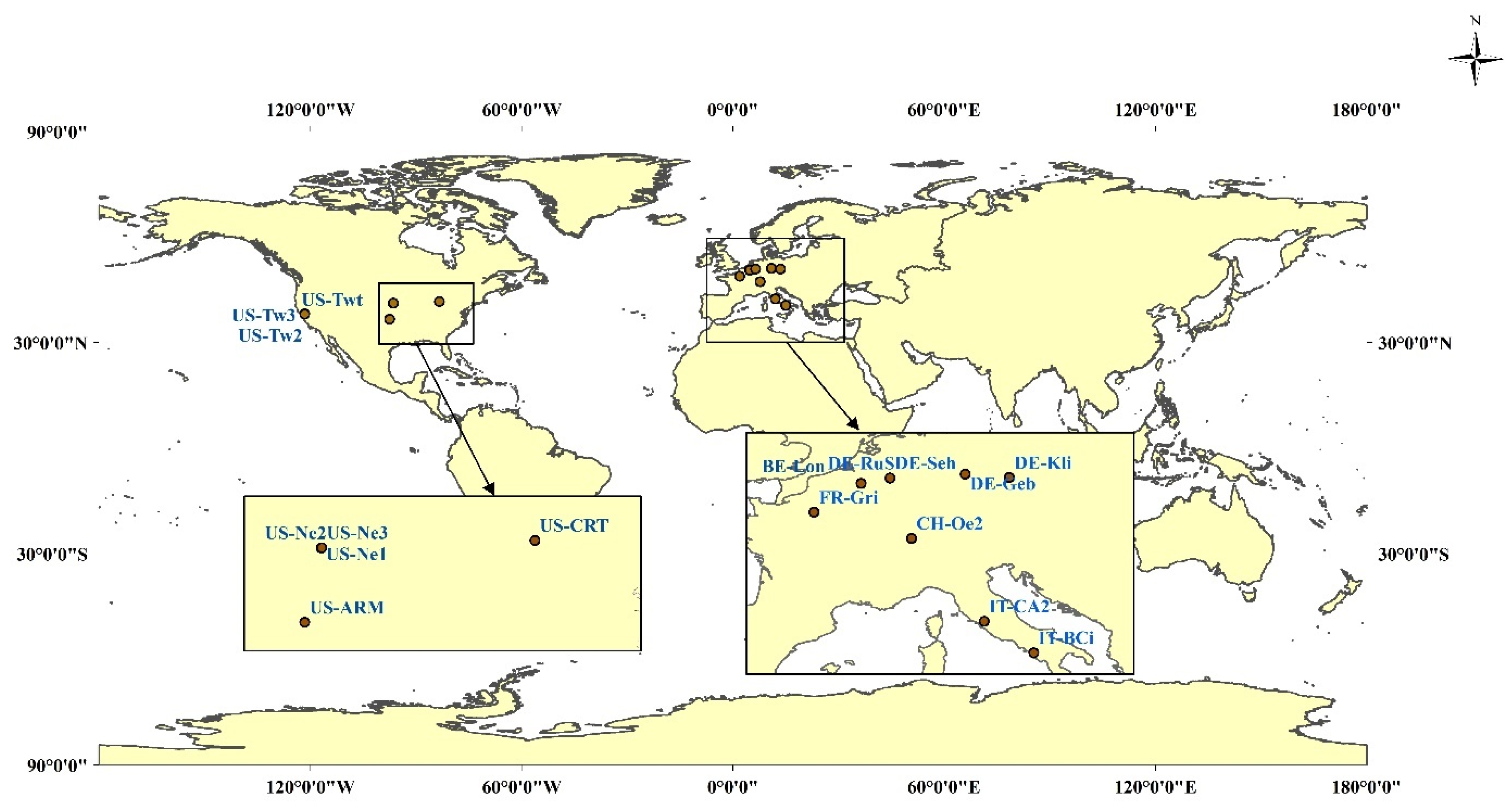
In this study, we used five meteorological factors’ data and observed ET data from the FLUXNET2015 dataset. Temporally continuous meteorological factors on a daily scale include temperature (Ta), precipitation (P), carbon dioxide concentration (Ca), solar radiation (SW) and vapor pressure deficit (VPD). They were retrieved from the meteorological observation data of the eddy covariance flux tower at 17 flux sites (Figure 1). These data are used as input parameters of the models and to build and verify models. Figure 1 shows the map representation of the 17 flux sites (see Appendix A for a detailed information of the 17 flux sites). The latitudes of all stations are between 36.60 (US-ARM) and 51.10 (DE-Geb) and the longitudes are between 121.65 and 14.96. DE-Kli and IT-BCi have the lowest (7.77 °C) and highest (17.88 °C) mean annual temperature, respectively. The annual precipitation of these sites varies from 343.10 mm to 2062.25 mm.
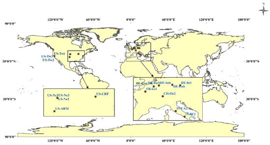
Figure 1.
Map representation of 17 eddy covariance flux site.
2.1.2. Remote Sensing Data
The remote sensing (RS) factors used in this study were from https://modis.ornl.gov/data.html (the date of accessing data is 27 February 2020), including normalized difference vegetation index (NDVI), enhanced vegetation index (EVI), near-infrared reflectance of vegetation (NIRv) and shortwave infrared band (SWIR). The time series of MODIS data were extracted according to the longitude and latitude coordinates of the flux sites in the Table 1. The spectral indices were calculated using the band reflectance provided by MCD43A4. The calculation formulas of NDVI, EVI and NIRv are as follows, and SWIR is calculated by using the reflectance data directly.
where NIR is Near Infrared band, Red is Red band, Blue is Blue band. NDVI is generally used to reflect the fractional cover of vegetation and has the ability to characterize the crop canopy [24]. EVI is more sensitive than NDVI to changes in canopy structure, and is used to optimize vegetation signals. NIRv, a RS measurement of canopy structure, is the product of NDVI and the total near-infrared reflectance (NIRt) (MODIS second band), and can predict photosynthesis accurately [25].

Table 1.
The different input combinations of the six ML algorithms.
2.2. Machine Learning-Based Models
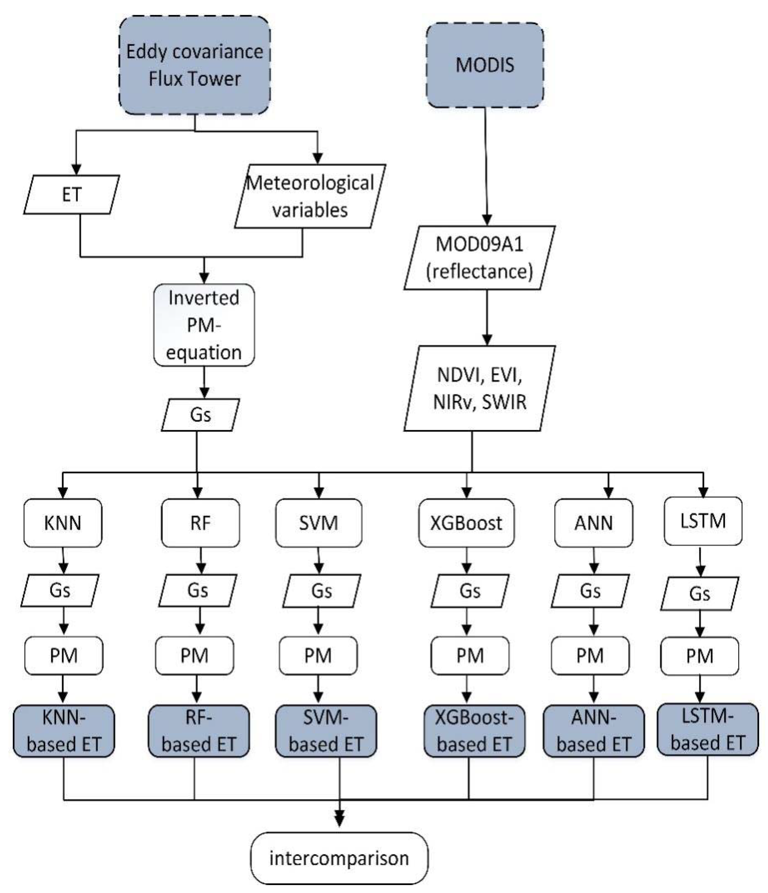
The flowchart of this study is shown in Figure 2. We evaluated six ML-based hybrid models to estimate cropland ET. The meteorological data and RS factors were input into the ML algorithms to construct the Gs model and the modeled Gs was incorporated into the PM equation to estimate ET. The ML algorithms include KNN, RF, SVM, XGboost, ANN and LSTM. Referring to Zhao et al. [17], we used the ML algorithms to model ln(Gs) rather than Gs, because the logarithmic form can effectively reduce the effect of errors in Gs calculated from the observations. Overviews of the six ML algorithms used in this study are presented in the following sections. The formula of the PM equation is as follows:
where is net radiation, is soil heat flux, is the gradient of the saturation vapor pressure versus atmospheric temperature, is air density, is the specific heat at constant pressure of air, is the vapor pressure deficit of the air, is the aerodynamic conductance and is the psychometric constant.

Figure 2.
Research flow chart. ET is evapotranspiration, Gs is surface conductance, PM is the Penman-Monteith equation, NDVI is normalized difference vegetation index, EVI is enhanced vegetation index, NIRv is near-infrared reflectance of vegetation and SWIR is shortwave infrared band. KNN is K nearest neighbor algorithm, RF is random forest, SVM is support vector machine, XGboost is extreme gradient boosting algorithm, ANN is artificial neural network and LSTM is long short-term memory. A white parallelogram denotes variable and a white rectangle denotes a method. A blue dotted rectangle denotes the source of the variable, and a gray solid rectangle denotes a model.
2.2.1. K Nearest Neighbor (KNN)
KNN is a theoretically mature non-parametric method [26]. It is easy to implement and is one of the simplest ML algorithms. The so-called K nearest neighbors means that each sample can be represented using its K nearest neighbors. After finding the K nearest neighboring values of sample X, the predicted value of the sample is obtained by calculating the average of these K neighboring values. A key of using the KNN method is the selection of the K value. The model will become complicated and prone to over-fitting if the K value is small. On the contrary, if the K value is large, the model is relatively simple. The prediction of the input instance of the model is not accurate, and the error is easy to become bigger. So, choosing an optimal K value is very important. In this study, the model was repeatedly trained, where the K value ranged from 1 to 30 and correlations coefficient (r) and bias of the corresponding model were output. The K value of corresponding model with a higher r and smaller bias was selected as the optimal K value.
2.2.2. Random Forests (RF)
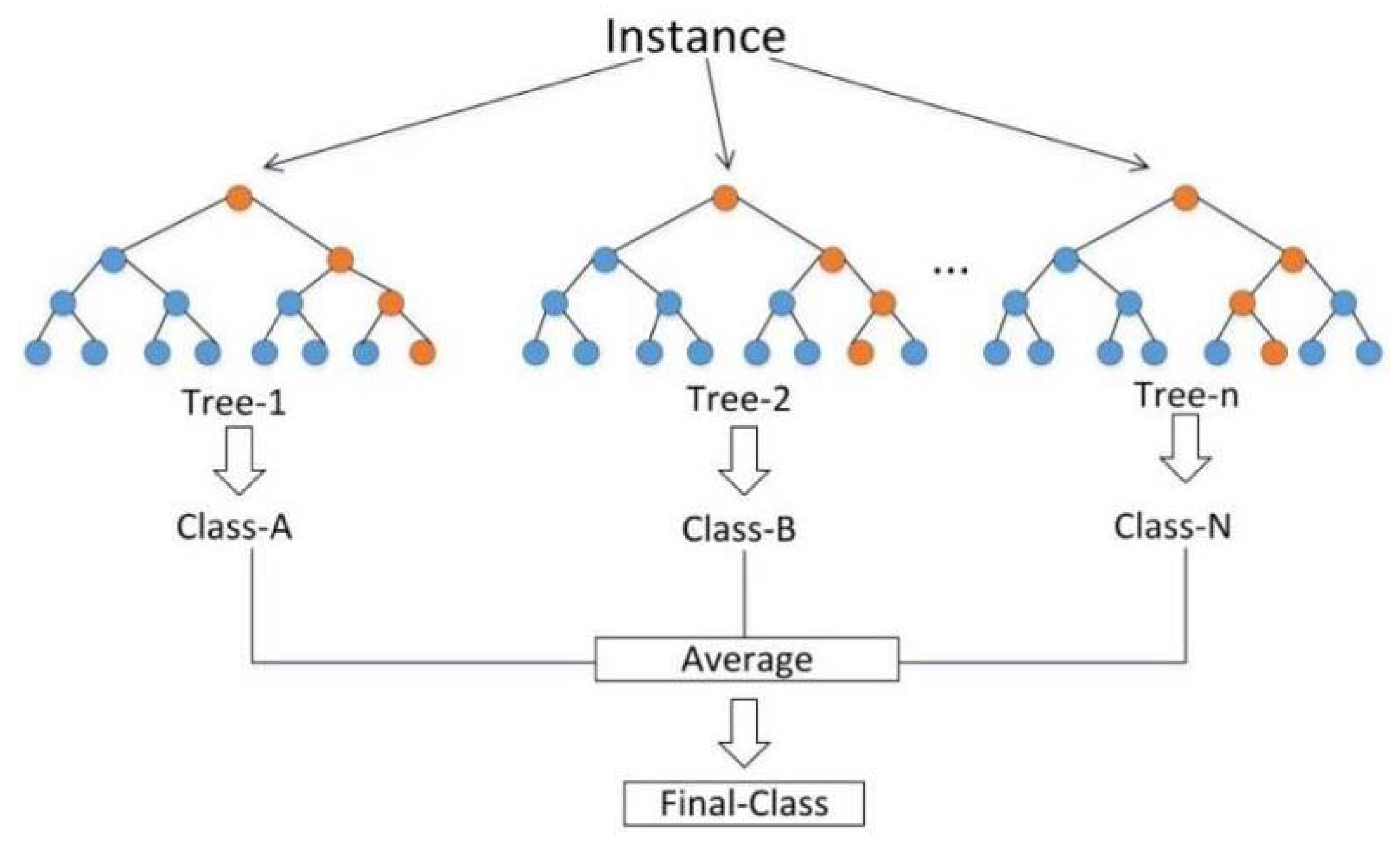
The RF algorithms was proposed by Breiman [27], a supervised learning algorithm that integrated multiple trees through the idea of ensemble learning. The idea of the RF is simple and easy to implement, and the computational cost is small. The decision rule of RF is shown in Figure 3. It is composed of multiple unrelated decision trees. Because each decision tree in RF has its own result, the final output result is determined by the average of the predicted values of multiple decision trees. Therefore, the performance of RF is generally better than that of a single decision tree. When training the RF model, we set the maximum depth (max_depth) of RF from 1 to 30 to repeat training the RF model in order to reduce the phenomenon of overfitting. The optimal max_depth of RF was selected by comparing r of the training and validation datasets models.
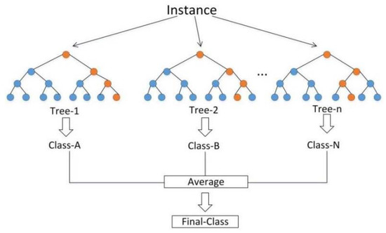
Figure 3.
The decision rule of RF model.
2.2.3. Support Vector Machine (SVM)
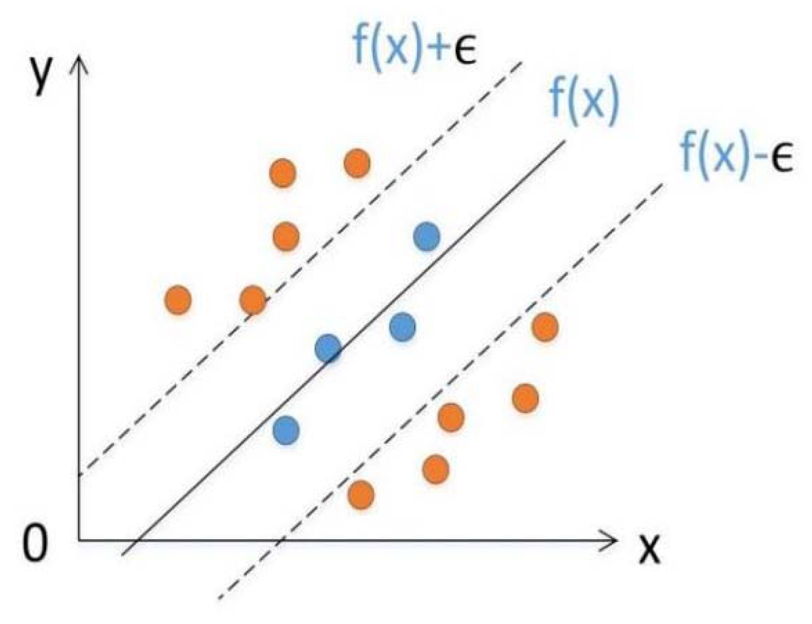
SVM is a ML algorithm proposed by Vapnik [28] to classify data in a supervised learning manner, and it can also perform regression analysis. The basic idea of SVM regression is to implement linear regression by constructing a linear decision function in a high-dimensional space after dimension upgrade. Figure 4 shows the basic idea of SVM regression, that is, to find a regression plane, so that all the data in a collection are the closest to the plane. It is equivalent to taking f(x) as the center and constructing a gap with width ϵ. If the training sample falls within this interval band, it is considered that the prediction is correct.
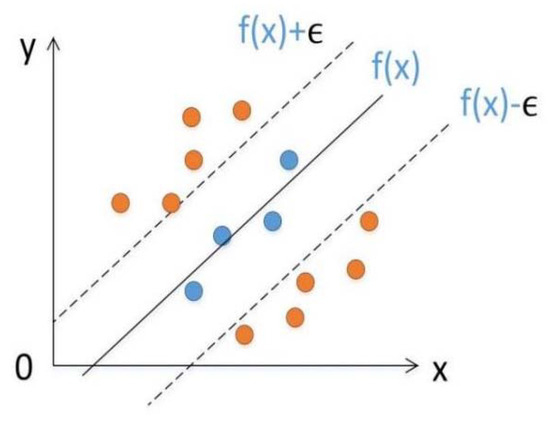
Figure 4.
The basic idea of SVM regression. Reference to Tinoco et al. [29].
2.2.4. Extreme Gradient Lift (XGboost)
XGboost is a new ML algorithm proposed by Chen and Guestrin [30], which uses gradient boosting as a framework and integrates many classification and regression trees. The so-called ensemble learning is to construct multiple weak classifiers to predict the dataset and then uses a certain strategy to integrate the results of the multiple classifiers as the final prediction result. The training speed of the XGboost is fast. Although there is a serial relationship between trees, nodes at the same level can be parallel. The core idea of the XGboost algorithm is to continuously add trees and continuously grow a tree by performing feature splitting. When the training is completed, k trees are obtained and then the score of a sample is predicted. Finally, the scores of corresponding to each tree are added up as the predicted value of the sample. Since XGboost is based on a tree model, the model was repeatedly trained, where max_depth value ranged from 1 to 30 to reduce overfitting when training the model. We selected the optimal max_depth through r of the training and validation datasets.
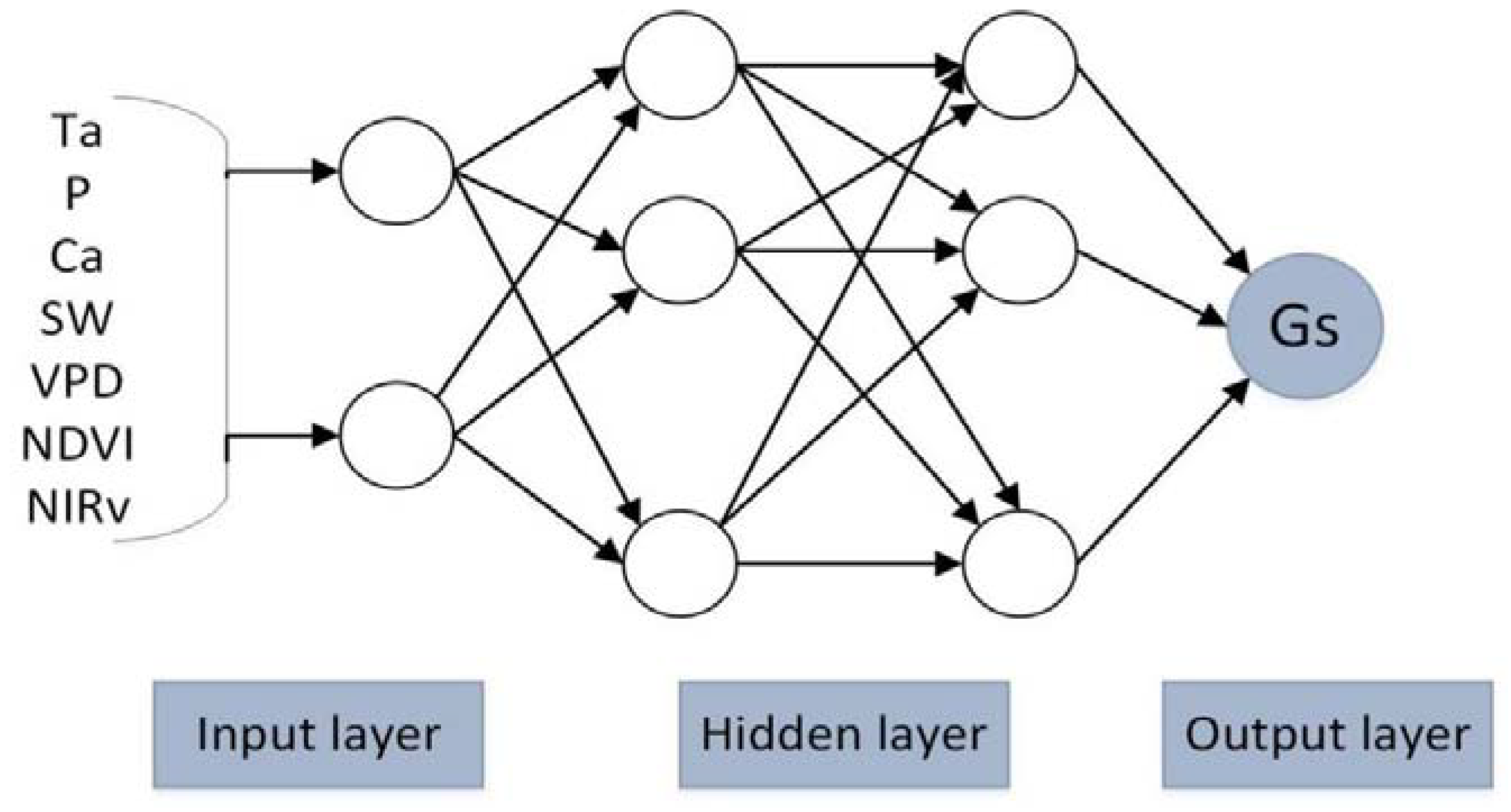
2.2.5. Artificial Neural Network (ANN)
Bruton et al. [31] developed the ANN model to estimate ET. ANN is a commonly used ML algorithm, and consists of a large number of nodes, called neurons, which are connected to each other. Each neuron has input and output connection. Figure 5 shows the three layers (input layer, hidden layer and output layer) structure of the ANN. The input layer is responsible for receiving input data from outside and transmit to the next layer, the hidden layer constructs the relationships between the input and output, and the output layer outputs the results. In order to reduce over-fitting, the model was repeatedly trained, where the number of hidden layers ranged from 1 to 10, and the number of neurons in each layer increased. Then, we selected the optimal network structure using the Akaike Information Criterion (AIC) and the evaluation parameter of the number of hidden layers-the number of neurons in the training and validation datasets. The calculation formula of the AIC indicator is as follows [32]:
where MSE is mean square error, is the number of observations in the training samples and is the total number of parameters in the network.

Figure 5.
The three layers structure of the ANN model. Ta is air temperature, P is precipitation, Ca is atmospheric carbon dioxide concentration, SW is solar radiation, VPD is vapor pressure deficit, NDVI is normalized difference vegetation index, NIRv is near-infrared reflectance of vegetation and Gs is surface conductance.
2.2.6. Long Short-Term Memory (LSTM)
The LSTM proposed by Hochreiter and Schmidhuber [33] is a special recurrent neural network with better performance in processing time series data. LSTM can learn long-term dependent information and solve vanishing gradient and exploding gradient problems in the process of long sequence training. LSTM consists of a large number of contiguous memory units and each memory unit has a unit state, three gates (input gate, output gate and forget gate) and hidden state. The input gate controls how much network’s input information is stored in the unit state, the output gate controls how much output value from the unit state is exported to the network and the forget gate determines whether the values in the unit state need to be forgotten. The network is repeatedly trained, where the number of hidden layers ranges from 1 to 10 and the number of neurons in each layer increases from 1 to 128, with an interval of 8. Finally, the optimal LSTM network structure is selected based on AIC.
2.3. Model Development
This study used meteorological data and RS factors to develop six hybrid ML-based ET models, which are supposed to be effective for estimating cropland ET on a regional scale. We divided the dataset into training dataset, validation dataset and test dataset to construct models of estimating ET, the proportions of which are 60%, 20% and 20%, respectively. Among them, the training dataset were used to fit data samples to train models, the validation dataset were used to adjust the parameters of the models and evaluate the ability of the models and the test dataset were used to evaluate the generalization ability of the trained models. In this study, we evaluated four different combinations of input factors to force the six ML-based models to estimate ET. The different input combinations of the six ML algorithms are shown in Table 1.
2.4. Model Evaluation
Two commonly model performance evaluation metrics were used to evaluate and compare the accuracy and performance of different models in estimating ET.
- Correlations coefficient (r): the value of r ranges between −1 and 1, with large values corresponding to a better performance. The calculation formula is as follows:where is the observed values, is the predicted values, is the average of observed values, . is the average of predicted values and is the total amount of experimental data.
- Root mean square error (RMSE): the value of RMSE ranges between 0 and positive infinity, with small values corresponding to a better performance. It is a measure of the difference between the predicted values and the observed values [34] and reflects the degree of dispersion of the predicted values to explain the true values. The calculation formula is as follows:
3. Results
3.1. Model Parameter Optimization
It is necessary to optimize the parameters of the models in the process of training models. Among them, the selection of K value in the KNN model, the max_depth of tree-based RF and XGboost models and the model structure of the ANN and LSTM models need to be optimized.
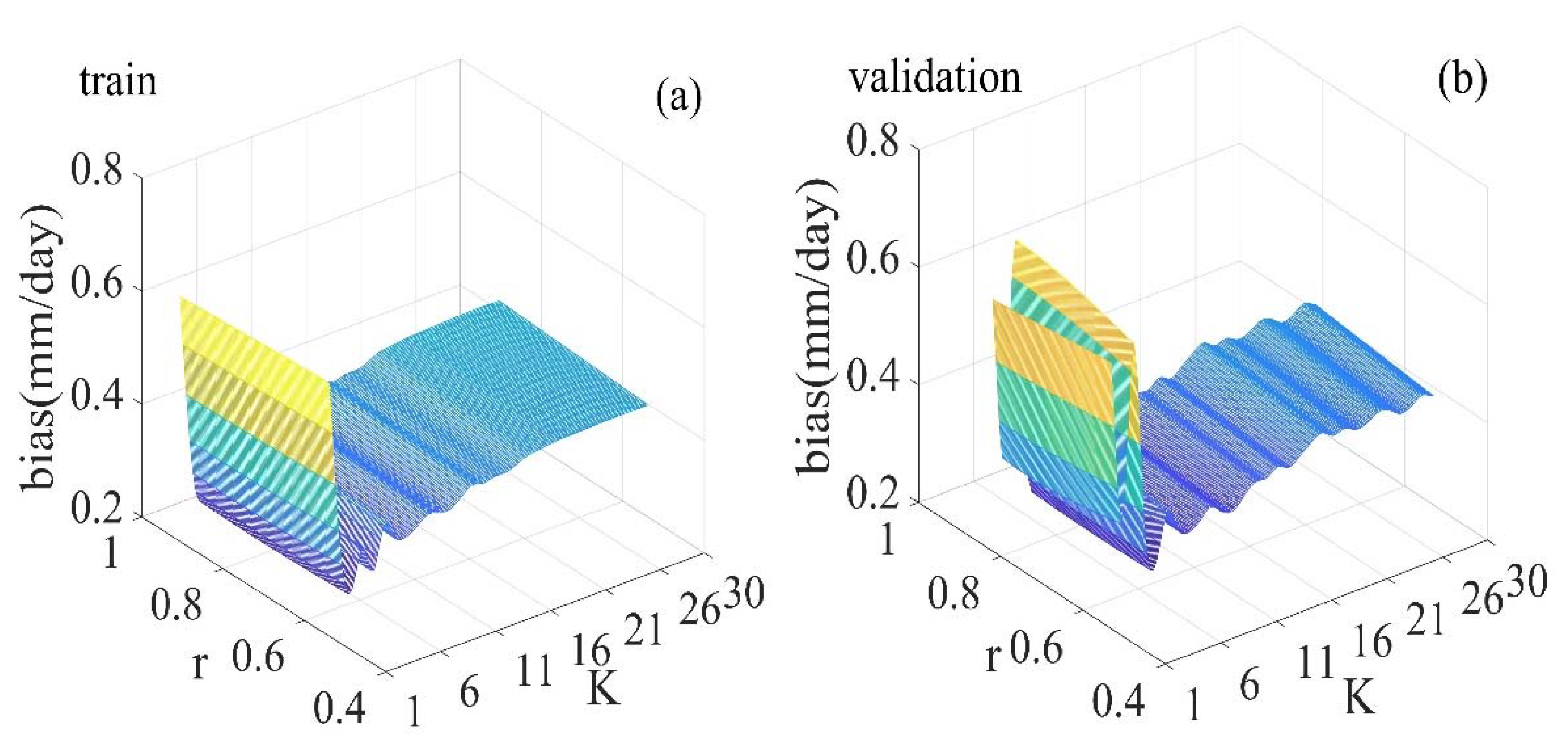
The key of training the KNN-based model is to determine the K value. The K value has a significant impact on the results of the KNN algorithm. Generally, the K value takes a smaller value. In this study, the KNN-based model was repeatedly trained, where the K value ranged from 1 to 30, to acquire the optimal K value. Figure 6 shows the three-dimensional graph between the K values, r and bias of the training and validation datasets of the KNN model. It can be seen that the r of the training dataset has an increasing trend as the K values increase, while the r of the validation dataset increases first and then decreases. The bias of the training and validation datasets fluctuate between 0.26 mm/day and 0.72 mm/day when K values are less than 11. The bias of the training and validation datasets show a gentle increasing trend when K values are greater than 11. The KNN-based model with a K value of 1 yielded the smallest r (0.54 and 0.53) for both training and validation datasets. The KNN-based model with a K value of 1 yields the largest bias (0.65 mm/day) for the training dataset, while the KNN-based model, with a K value of 3, yields the largest bias (0.72 mm/day) for the validation dataset. The K value of 5 was identified as the optimal, as the model with this K value yielded the best performance with r = 0.80 and 0.82 and bias = 0.28 mm/day for training and validation datasets.
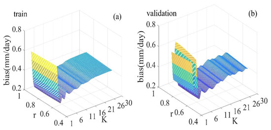
Figure 6.
The three-dimensional graph between the K values, r and bias of the training and validation datasets of the KNN-based model. R2 is the correlations coefficient. (a) is the three-dimensional graph between the K values, r and bias in the training dataset, (b) is the three-dimensional graph of the validation dataset.
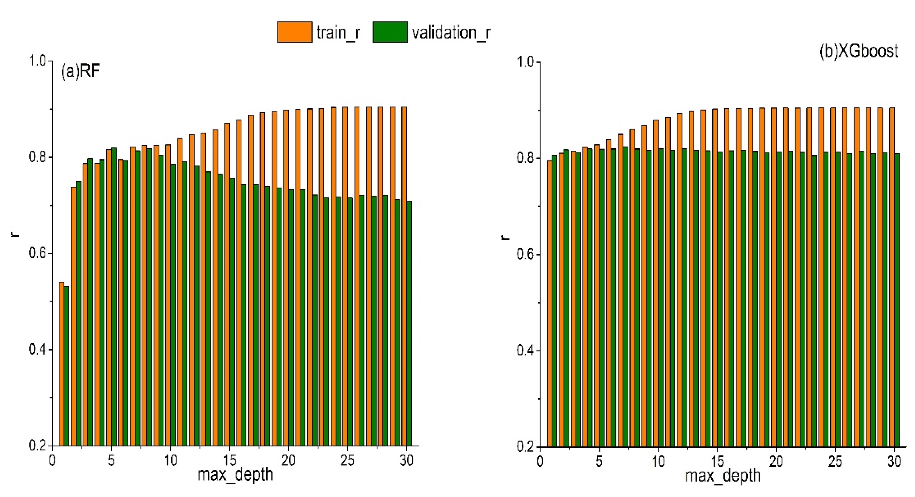
Some parameters of the RF-based model need to be adjusted in order to prevent overfitting. Properly adjusting the max_depth of the tree can reduce the complexity of the learning models, as well as the risk of overfitting and thus help to obtain the best results. In this study, the RF-based model was repeatedly trained, where the max_depth ranged from 1 to 30, to find the optimal max_depth value. Figure 7 shows the variations in r of RF and XGboost for both validation and training with the changes of max_depth. In the sub-picture (a), the r of the training dataset keeps increasing and the r of the validation dataset increases first and then decreases as the max_depth increase. The performance of the RF-based model is the worst when max_depth is 1, with the smallest r of 0.54 and 0.53 for training and validation datasets, respectively. The difference in r between training and validation datasets reached the largest values at max_depth of 30. The r of the training dataset is 0.80 and the r of the validation dataset is 0.79 when max_depth is 6. The difference in r between training and validation datasets at max_depth of 6 is the smallest and the difference in r between training and validation datasets with max_depth of 8 is roughly the same as max_depth is 6. Since r is higher when max_depth is 8, the optimal max_depth selected in this study is 8. XGboost is a tree-based algorithm, and the parameter optimization process is similar with that of the RF algorithm. For example, the sub-picture (b), the r of the training dataset shows an increasing trend as the max_depth increase and the r of the validation dataset starts to decrease slowly after peaking at max_depth of 7. Therefore, the optimal max_depth for XGboost recognized as 7 in this study. Based on the AIC values, we identified the best architectures of ANN and LSTM have two hidden layers and the number of neurons in each layer is 48 and 40, respectively. Table 2 shows the optimal parameters of the KNN-based model, RF-based model, XGboost-based model, ANN-based model and LSTM-based model.
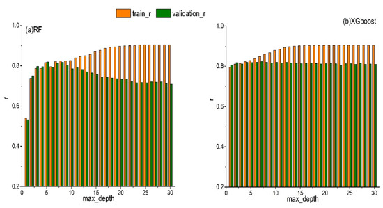
Figure 7.
r values of RF (a) and XGboost (b) models for training (orange bars) and validation (green bars) with max_depth changing from 0 to 30. r is the correlations coefficients and max_depth is the maximum depth of tree.
Table 2.
The optimal parameters of the KNN-based model, RF-based model, XGboost-based model, ANN-based model and LSTM-based model.
3.2. Comparison of Six ML Algorithms for Estimating Gs with Different Combinations of Input Variables
In our study, we use ML algorithms to model Gs, and then estimate ET based on PM equation and the ML-based Gs. Table 3 shows the performance (r, significance level) of the six types of ML-based Gs models with ten different input combinations. In the all types of ML-based Gs models with ten different input combinations, the ANN-based model with the combination 10 has the best performance (r = 0.70, significance level is ***), and the KNN-based model with the combination 4 has the worst performance (r = 0.34, significance level is ***). ML-based Gs models with combinations 8–10 produce similar and relatively high accuracy (r = 0.47–0.70, significance level are ***), with the exceptions of LSTM-based models. However, the ML-based Gs models with combinations 1–4 have the lowest r (0.34–0.66) and significance level are all ***, and the models with combinations 5–7 present intermediate results. As for the LSTM-based models, the models with combination 1 and 2 yield the best performance (r = 0.62, significance level are ***) and the worst performance (r = 0.47 and significance level is ***) with input combination 3. Among the six types of ML-based Gs models with the combination 1-9, ANN-based models have the highest accuracy, with higher r (0.65–0.70) and significance level are all ***, followed by the LSTM-based models. In contrast, the KNN-based models have the lowest r (0.34–0.48) and significance level are all ***. With the combination 10, similarly, ANN-based model has the highest r = 0.70 and significance level is ***, followed by XGboost-based model and KNN-based model has the lowest accuracy (r = 0.48, significance level is ***) and the performance of LSTM-based model is reduced (r = 0.52, significance level is ***). The significance level between the observed and predicted Gs in the test dataset of six ML-based hybrid models are ***, indicating that they are significantly correlated.
Table 3.
The Comparisons between the Predicted Gs and the observed Gs in the test dataset of six ML-based hybrid models corresponding to different input combinations. The input data of the combination 1–10 are shown in Table 1. The values in Table are correlations coefficient (r) and all r values reach the same significance level (0, ***).
3.3. Accuracy of Hybrid Models with Different Combinations of Input Variables
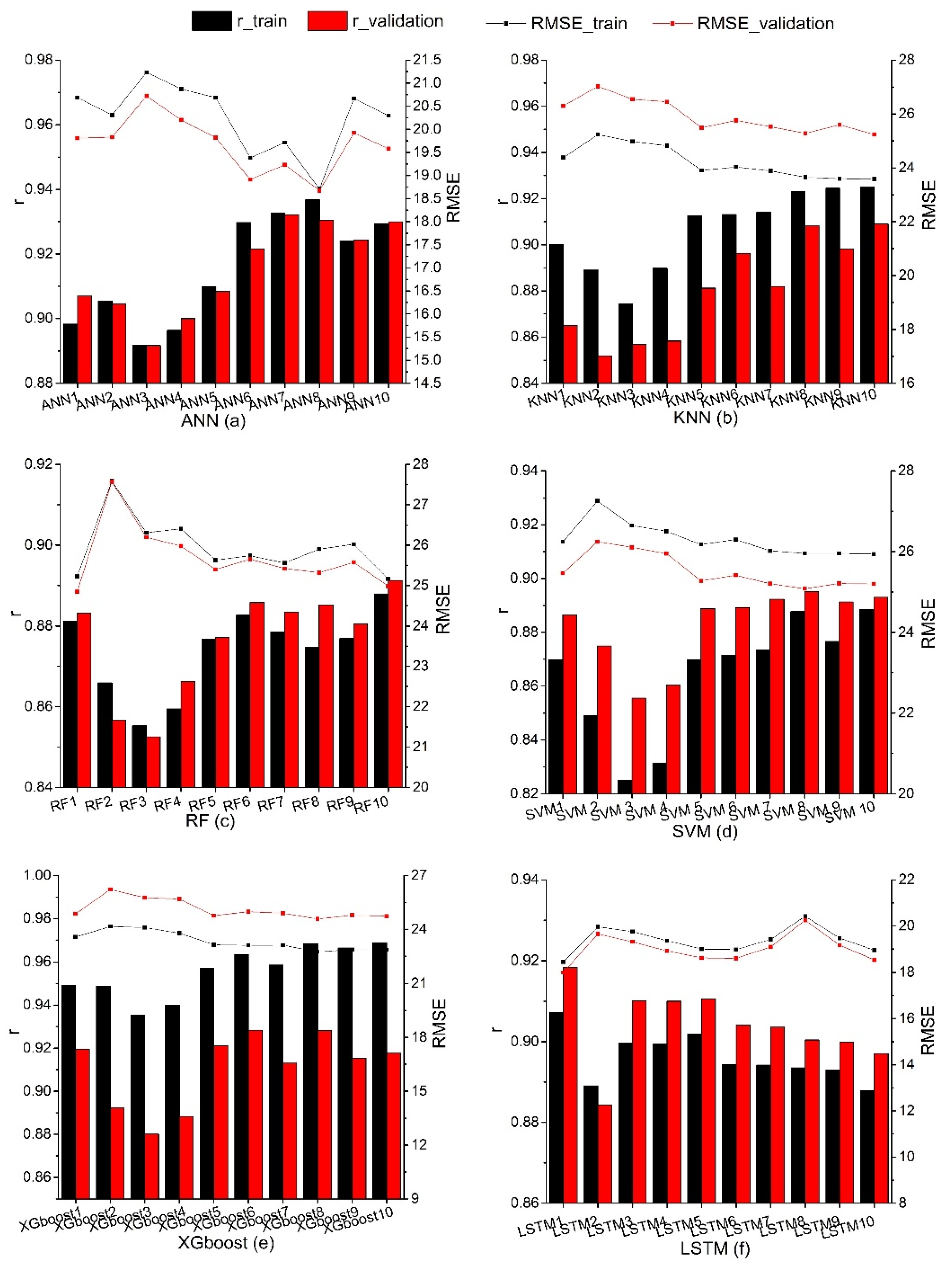
In this study, ten different input variables in Table 1 were input into six ML algorithms to construct Gs and then the PM equation was used to estimate ET. The line charts of the RMSE and r of the training and validation datasets of ten different hybrid models corresponding to various ML algorithms are shown in Figure 8. It can be seen that the evaluation metrics (RMSE and r) of the training and validation datasets show the similar trend. For the first four input combinations, the RMSE of the ANN3 (20.72–21.23 W m−2) and ANN2 (19.81–20.31 W m−2) hybrid models reach the maximum and minimum values, respectively. The RMSE values of other five models reach the maximum and the minimum values at the second (19.65–27.59 W m−2) and first (18.00–26.40 W m−2) input combinations, respectively. As far as r is concerned, the third input combination exhibits the worst performance (0.82–0.90) over all hybrid models except for LSTM, which performs the worst for the second input combination (0.88–0.89). The r of the first input combination achieves the maximum value (0.86–0.95) in the all hybrid models. When using one RS factor, SWIR has a greater advantage for the ANN-based hybrid model. For the other five hybrid models, NDVI has a higher advantage.

Figure 8.
The line chart of the RMSE and r of the training and validation datasets of ten different hybrid models corresponding to various ML algorithms. (a) is the line chart of the RMSE and r of the training and validation datasets of ANN model, (b) is the KNN model, (c) is the RF model, (d) is the SVM model, (e) is the XGboost model, and (f) is the LSTM model. RMSE is the root mean square error.
In the input combinations using two RS factors, KNN6, RF6, SVM6 and XGboost6 have the highest RMSE (24.03–26.29 W m−2) and ANN6 and LSTM6 have the lowest RMSE (18.60–19.38 W m−2). For the r, the r of ANN and SVM show an increasing trend, LSTM show a decreasing trend, but KNN, RF and XGboost first increase and then decrease. In general, the performance of the fifth and seventh input combination hybrid models has the similar results when two RS factors are used in the hybrid models. Compared with the eighth and ninth input combination hybrid models, the RMSE of the hybrid models shows an increasing trend except for LSTM, which is a decreasing trend, but r keeps decreasing. The eighth input combination hybrid models (KNN, RF, SVM, XGboost, ANN and LSTM models) have the smaller RMSE (18.67–25.96 W m−2) and higher r (0.87–0.97) and have higher performance of estimating ET. The tenth input combination hybrid model uses four RS factors. It has the lowest RMSE (22.85–25.24 W m−2) and the highest r (0.89–0.92) among the KNN and RF-based hybrid models. In the ANN, SVM and XGboost-based hybrid models, the eighth input combination hybrid model achieved the best performance (RMSE = 18.67–25.96 W m−2, r = 0.89–0.97). In the LSTM-based hybrid model, however, the first input combination hybrid model has the lowest RMSE (18.00–28.91 W m−2) and the highest r (0.85–0.92).
In general, the performance of the five ML-based hybrid models, except for LSTM using the four RS factors, is relatively better. The five ML-based hybrid models of using one RS factor show the largest RMSE and smallest r in all hybrid models. However, the LSTM-based hybrid model using a NDVI RS factor has the best performance. The LSTM model with the second input combination has the highest RMSE and lowest r. In the six hybrid models, compared with the hybrid models with two RS factors, the results of the hybrid models using three or four RS factors are similar and the accuracy of the hybrid models are not much different.
3.4. Comparison of ML-Based Hybrid Models
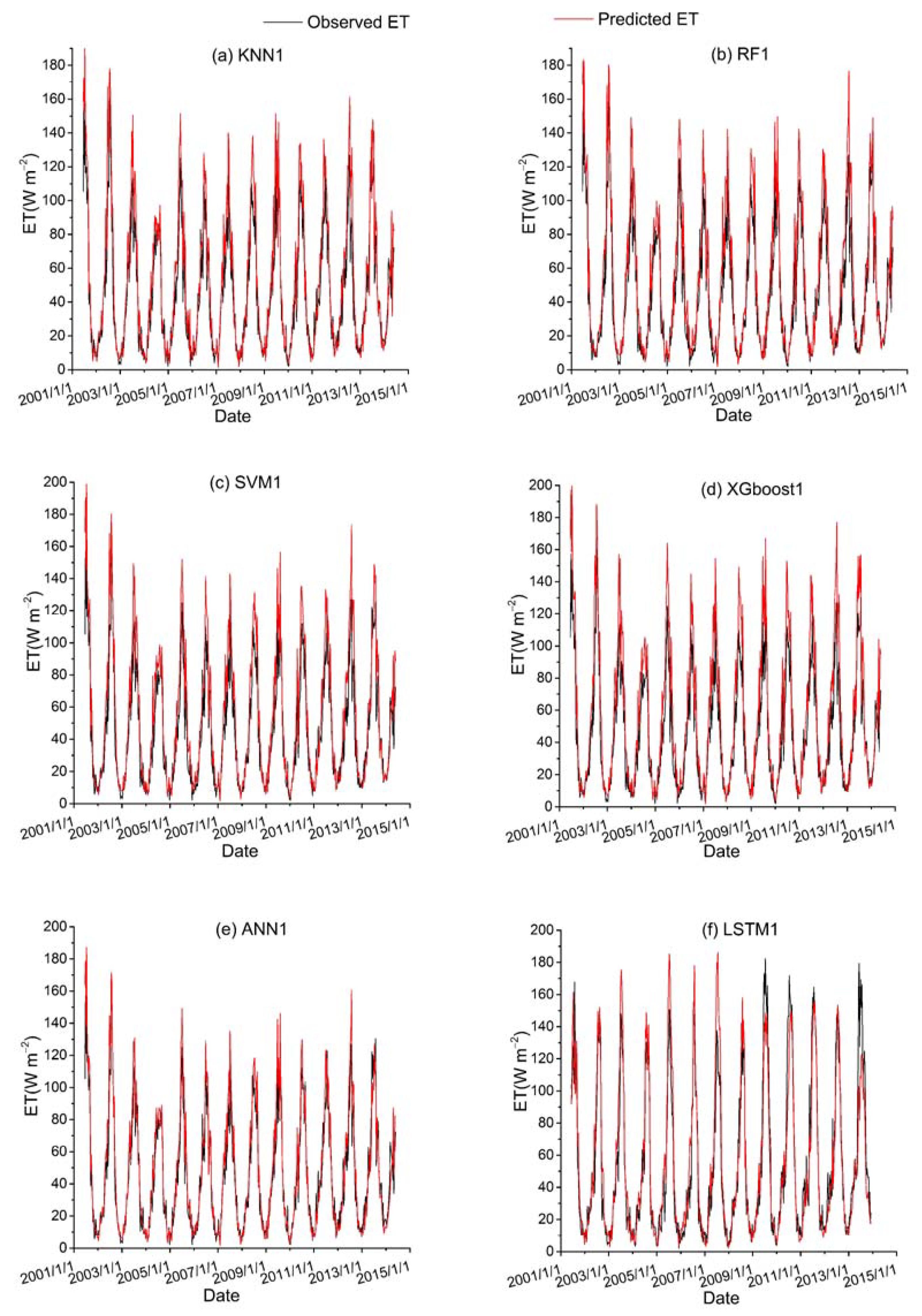
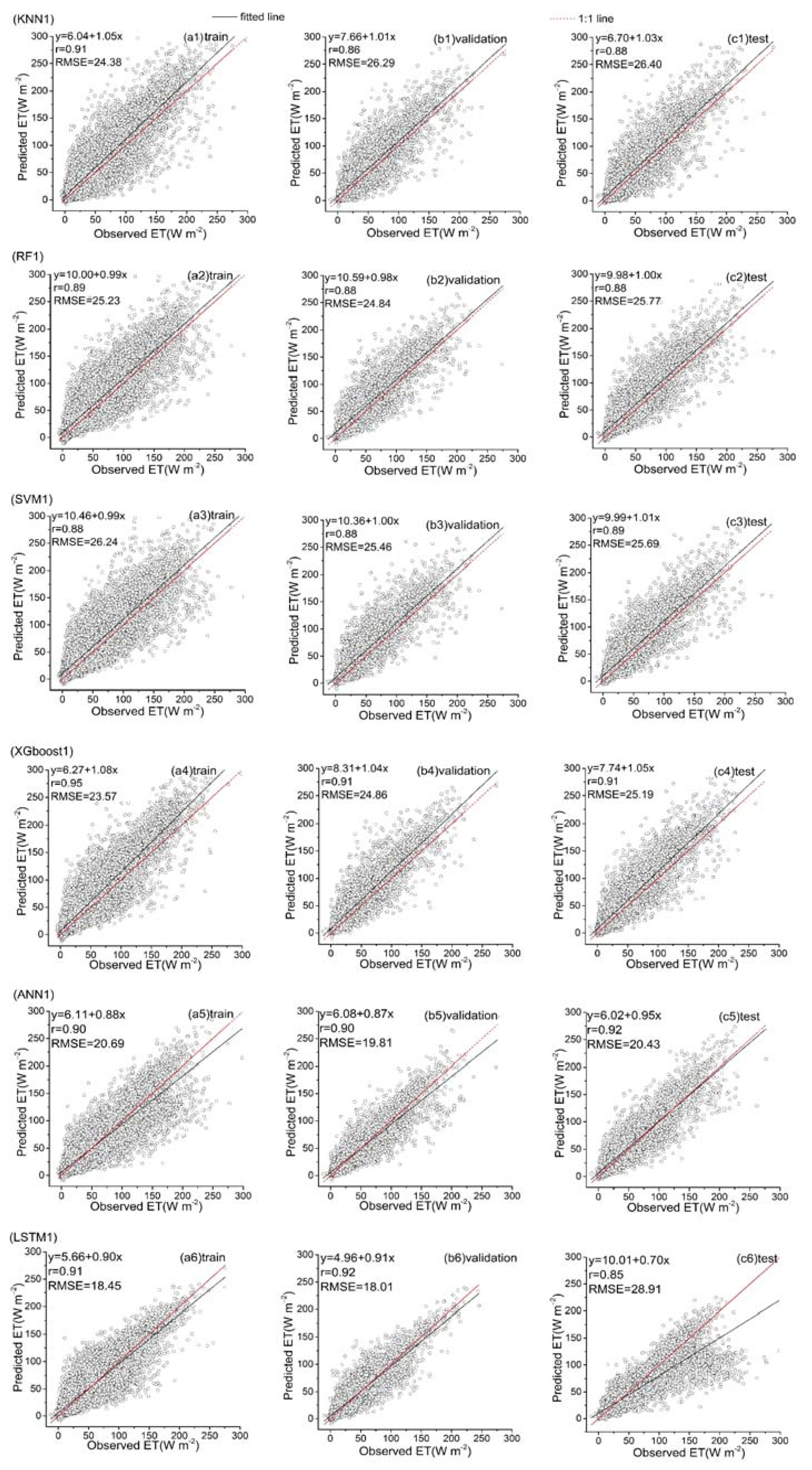
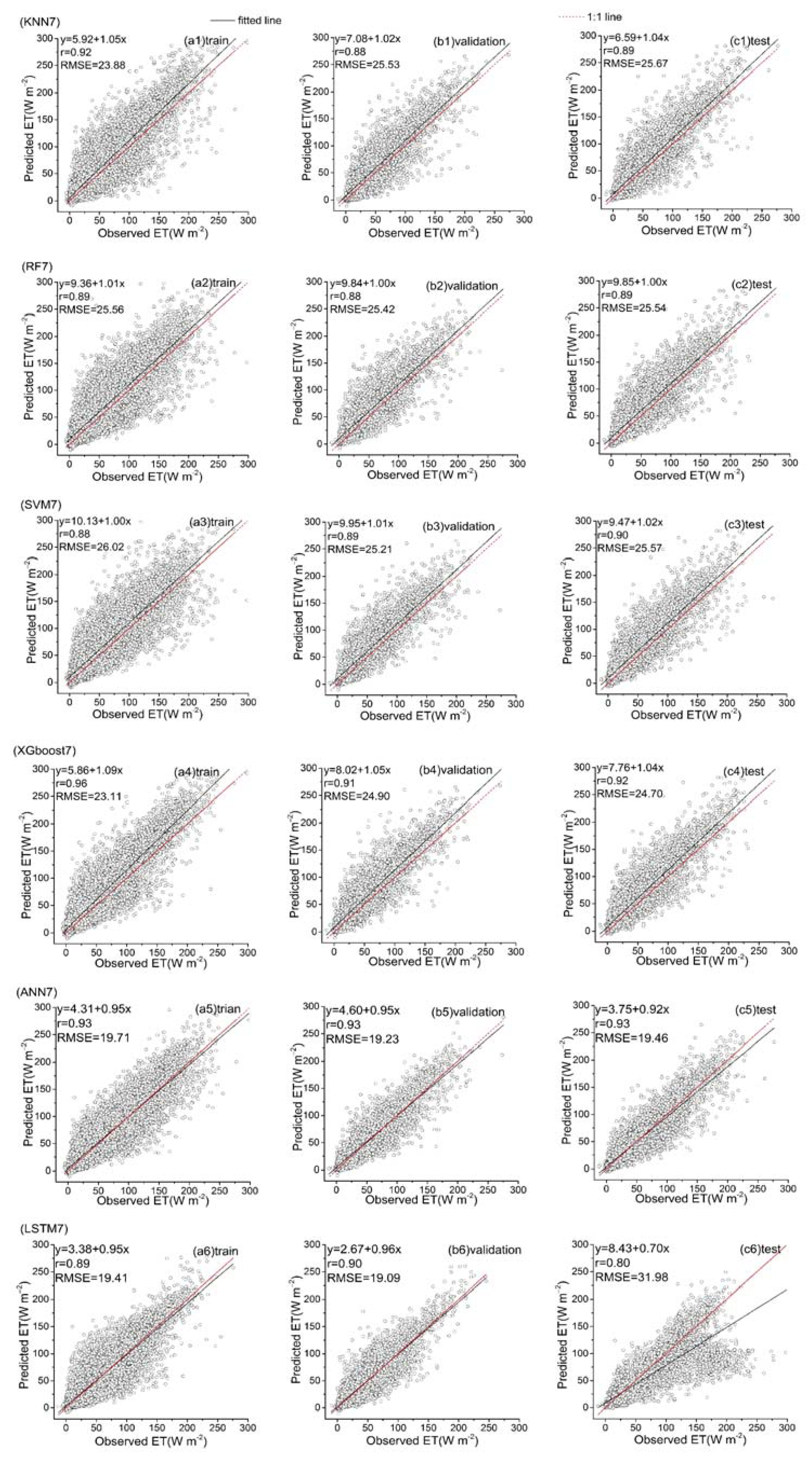
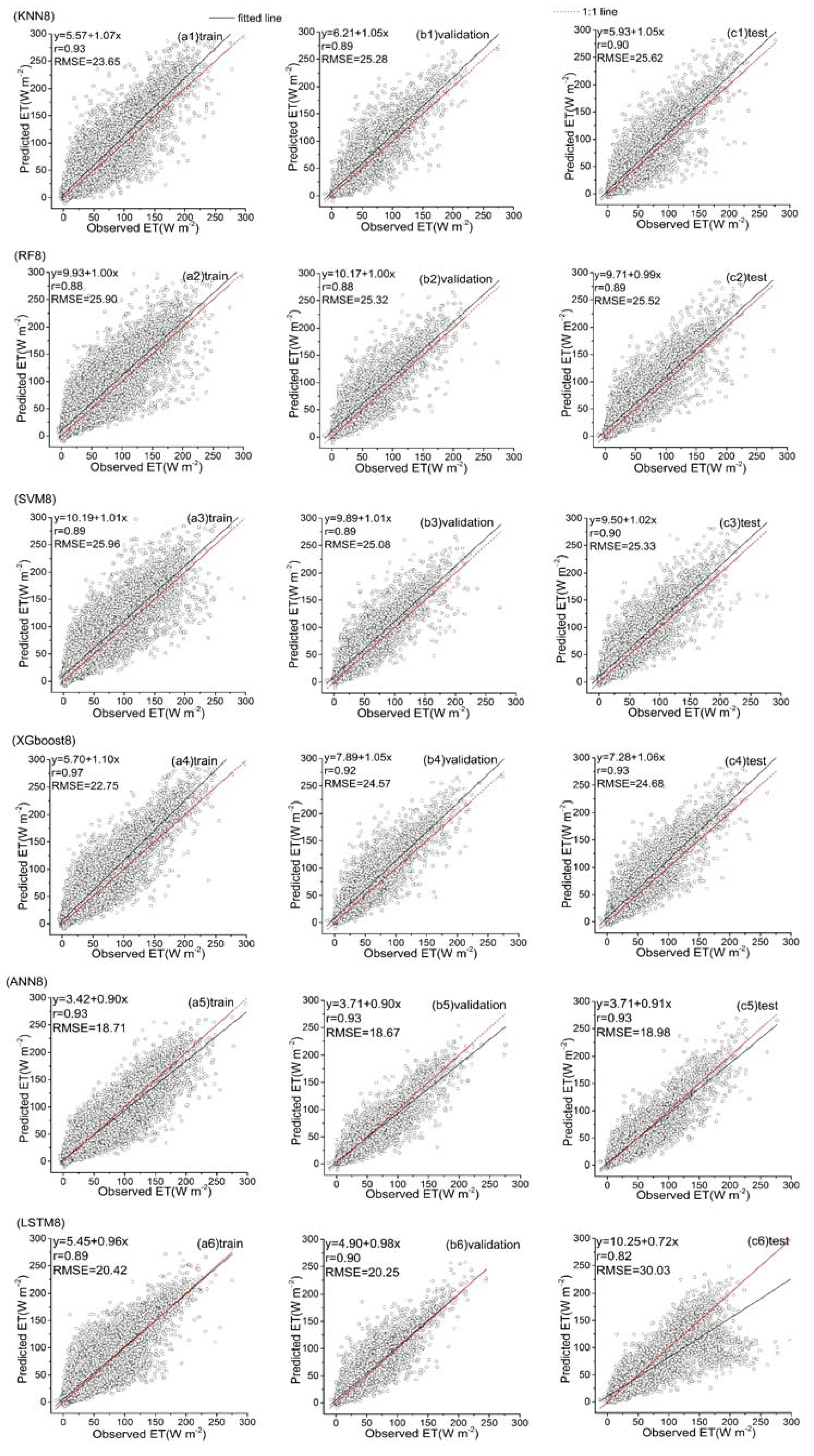
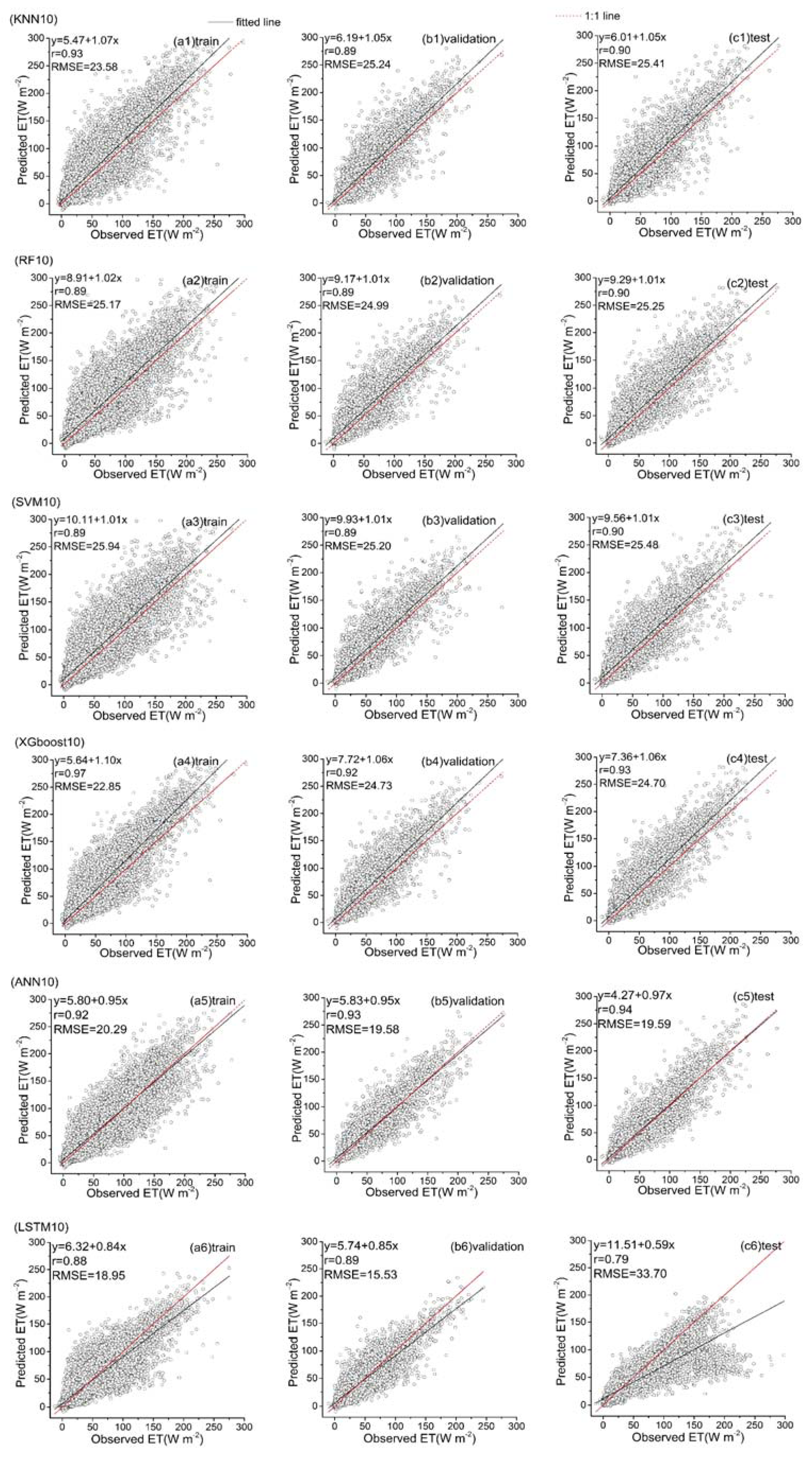
Among all the hybrid models of the six ML-based methods, we selected four hybrid models of input combinations to compare the performance of various ML-based hybrid models in estimating ET. The first input combination is model1 (meteorological data and one RS factor NDVI), the second input combination is model7 (meteorological data and two RS factors (NDVI, NIRv)), the third input combination is model8 (meteorological data and three RS factors (NDVI, NIRv, SWIR)) and the fourth input combination is model10 (meteorological data and four RS factors). Figure 9, Figure 10, Figure 11 and Figure 12 show the time series diagrams of observed ET (black line) and predicted ET (red line) over the test dataset for the six ML-based hybrid models corresponding to four input combinations. Figure 13, Figure 14, Figure 15 and Figure 16 show the comparisons between the predicted ET and the observed values of estimating cropland ET in the training, validation and test datasets of the six ML-based hybrid models corresponding to four input combinations. In all hybrid models, ET predicted by the ANN-based model agrees well with the observations, indicating that the ANN-based model can well capture the time series changes of ET and shows the best performance with the highest accuracy, followed by the performance of the XGboost-based model and the performance of the other three hybrid models (KNN-based, RF-based and SVM-based) are similar. The SVM-based model has better ability to capture the time series changes of ET and higher performance (r = 0.88–0.89, RMSE = 25.46–26.24 W m−2) to estimate ET than that of KNN and RF-based models when meteorological data and one RS factor (model1) are used in the models. The performance of the KNN-based model (r = 0.86–0.91, RMSE = 24.38–26.40 W m−2) is the lowest and the ability of capturing the time series changes of ET is the worst. Additionally, the RF-based model shows intermediate results. The performance of all hybrid models using two RS factors are improved compared with using one RS factor and the ability of all hybrid models using two RS factors to capture the ET time series changes are higher than the models using one RS factor. The r of the RF-based and SVM-based models using three RS factors are not improved, and the RMSE decreases more than those using two RS factors. The performance (RMSE =23.58–25.62 W m−2, r = 0.89–0.93) of estimating ET and the ability to capture the ET time series changes of the KNN-based model using three or more RS factors is only marginally better than those using two RS factors. Compared to use three RS factors, the RMSE (25.20–25.94 W m−2) of the SVM-based model is increased, the performance of the SVM-based model of estimating ET decreases and the ability to capture the time series changes of ET becomes weak when all RS factors are added to the model. The performance of estimating ET and the ability to capture the ET time series changes of the KNN-based and RF-based models using all RS factors is only marginally better than those using three RS factors. In the all hybrid models, the LSTM-based hybrid model has the worst ability to capture the time series changes of ET. The LSTM-based hybrid model of the training and validation datasets has a better performance with RMSE = 18.00–20.42 W m−2 and r = 0.88–0.92. However, the performance of the LSTM model of the test dataset is low (RMSE = 28.08–33.93 W m−2, r = 0.79–0.85).
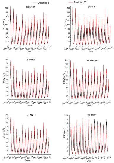
Figure 9.
Time series diagrams of observed ET (black line) and predicted ET (red line) over the test dataset for six ML-based hybrid models (KNN1, RF1, SVM1, XGboost1, ANN1 and LSTM1) that used the first data combination (see Table 1).
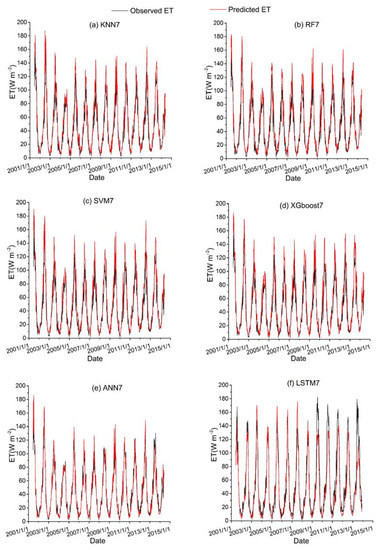
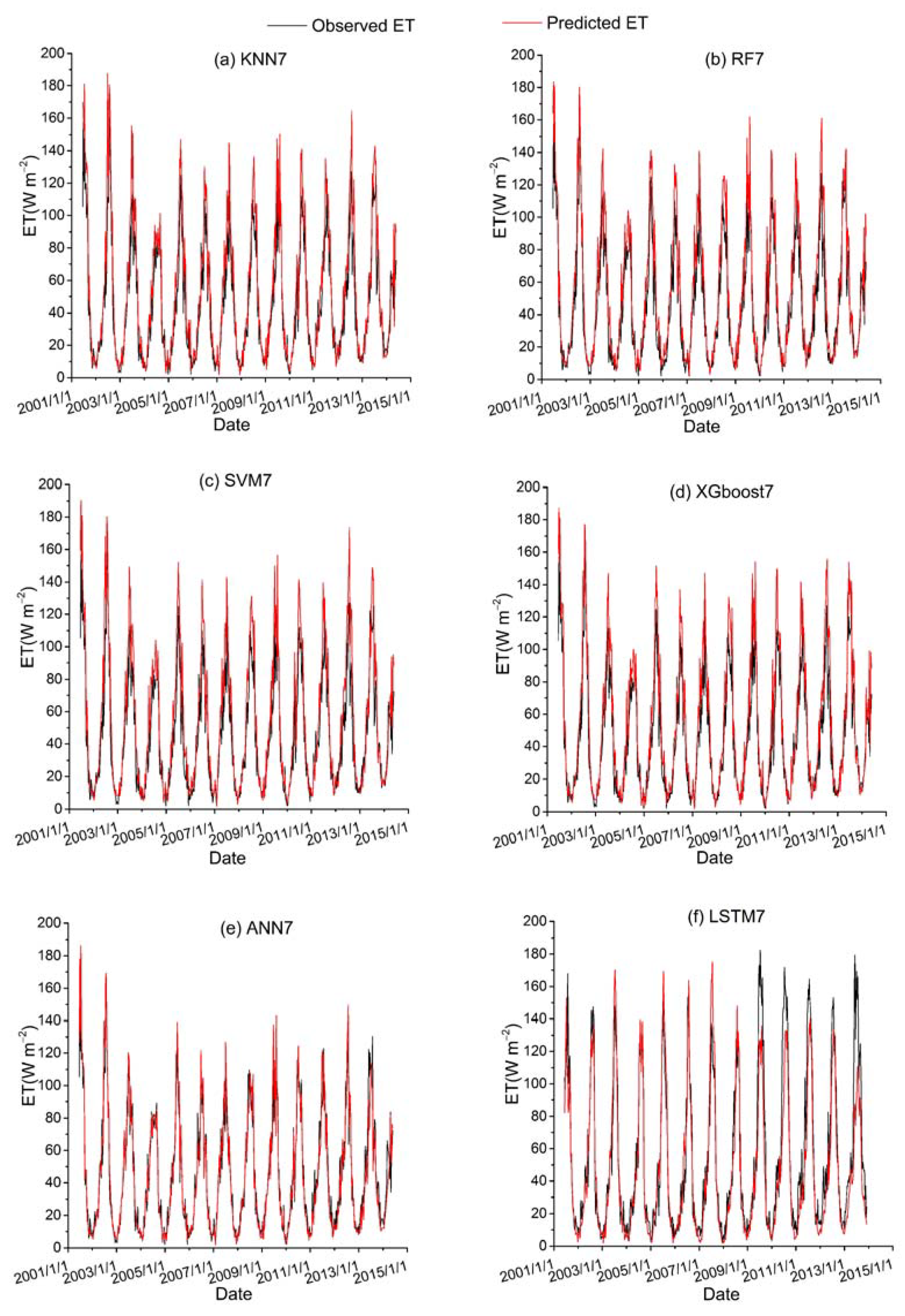
Figure 10.
Time series diagrams of observed ET (black line) and predicted ET (red line) over the test dataset for six ML-based hybrid models (KNN7, RF7, SVM7, XGboost7, ANN7 and LSTM7) that used the second data combination (see Table 1).
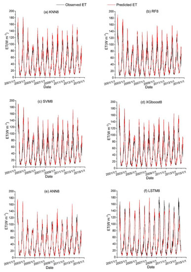
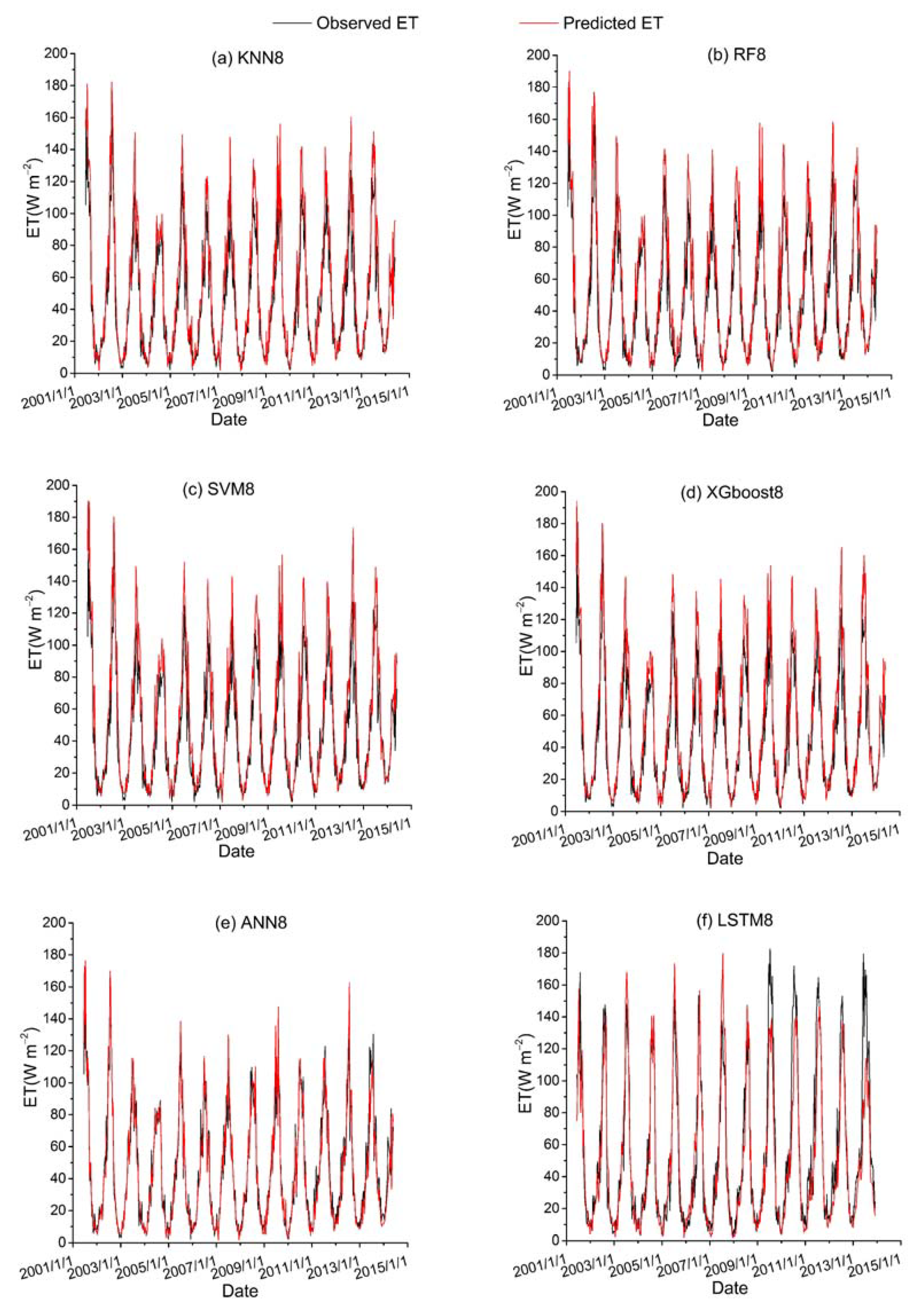
Figure 11.
Time series diagrams of observed ET (black line) and predicted ET (red line) over the test dataset for six ML-based hybrid models (KNN8, RF8, SVM8, XGboost8, ANN8 and LSTM8) that used the third data combination (see Table 1).
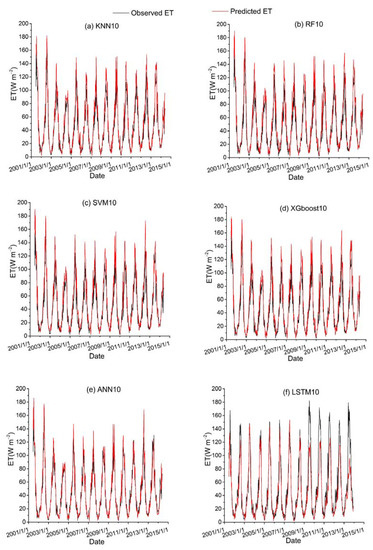
Figure 12.
Time series diagrams of observed ET (black line) and predicted ET (red line) over the test dataset for six ML-based hybrid models (KNN10, RF10, SVM10, XGboost10, ANN10 and LSTM10) that used the fourth data combination (see Table 1).
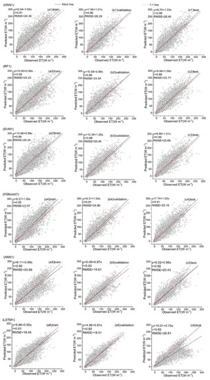
Figure 13.
Predicted ET vs. the observed values over the training, validation and test datasets for six hybrid ET models (KNN1, RF1, SVM1, XGboost1, ANN1 and LSTM1) that used the first data combination (see Table 1).
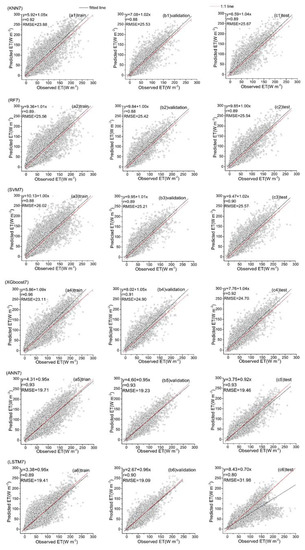
Figure 14.
Predicted ET vs. the observed values over the training, validation and test datasets for six hybrid ET models (KNN7, RF7, SVM7, XGboost7, ANN7 and LSTM7) that used the second data combination (see Table 1).
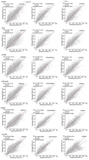
Figure 15.
Predicted ET vs. the observed values over the training, validation and test datasets for six hybrid ET models (KNN8, RF8, SVM8, XGboost8, ANN8 and LSTM8) that used the third data combination (see Table 1).
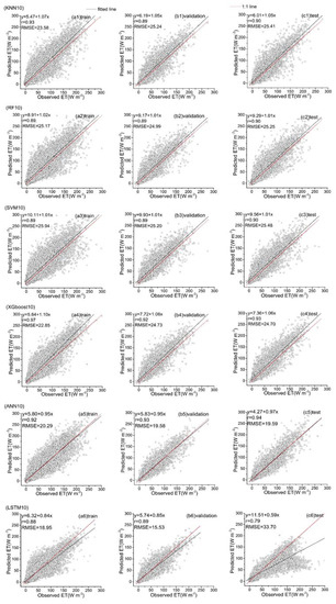
Figure 16.
Predicted ET vs. the observed values over the training, validation and test datasets for six hybrid ET models (KNN10, RF10, SVM10, XGboost10, ANN10 and LSTM10) that used the fourth data combination (see Table 1).
4. Discussion
4.1. Comparison of This Study with Other Studies
The six ML-based hybrid models evaluated in this study have good performances in estimating cropland ET. Among them, the ANN-based hybrid model has the best performance compared to other models, followed by the XGboost-based and KNN-based hybrid models and the RF-based and SVM-based hybrid models show intermediate results. The last is the LSTM-based model. In this study, the ET hybrid models combining the ML algorithm and PM equation show improved performance as compared to only use PM equation [35]. At the same time, the combination of easily available meteorological data and RS factors further enhanced the advantages of the ML-based hybrid models in estimating ET. However, it should be noted that the performance of the ML-based hybrid models could vary with difference in study regions and methods, input data, temporal scale of validation and so on. Table 4 shows the comparison of this study with other studies. For example, ML-based models generally showed higher r compared to using only the PM equation. Compared with only using meteorological data, the models that introduce RS factors can yield better performance metrics (RMSE, r). The models of using some data that are easy to obtain have greater advantage than that are difficult to get. The performance of the models targeting reference ET is higher compared to the targeting actual ET, as reference ET depends on only a few meteorological data [17,22,23,35,36].
Table 4.
Comparison of this study with other studies.
4.2. Reasons for Poor Performance of LSTM-Based Model
LSTM is a cyclic neural network architecture, which is very suitable for time series data. In most studies, LSTM model can effectively improve the accuracy of predicting future ET [37,38,39]. In this study, however, we find that the performance of the LSTM-based model in estimating ET time series is not as good as that of other ML-based models, as the r and RMSE values of the LSTM-based model are not statistically high. There may be two reasons for such results. Firstly, the advantage of LSTM lies on predicting the future ET by analyzing the relationship between the historical values of input variables and the target value in the future. Other ML models simulate the relationship between the current values of input variables and the current target value. Therefore, the reason for the poor performance of LSTM may be that the dominant factor of ET is the meteorological factor and remote sensing factor at the current time. Secondly, the performance of the model varies as the regions change [40,41].
4.3. Uncertainty of Machine Learning Algorithm
ML algorithms have been widely used in the estimation of ET. Most of them are black box models, without any physical basis, which may induce uncertainty in the resultant. In addition, for using the ML-based models to estimate ET, different input combinations will also affect the accuracy of ET models simulation results. Antonopoulos and Antonopoulos [18] used ANN and some empirical methods to estimate ET with daily meteorological data. The results showed that the model using three input variables (R = 0.952–0.978, RMSE = 0.598–0.954 mm d−1) had better performance in estimating ET compared with the models using two input variables (R = 0.910–0.956, RMSE = 0.846–1.326 mm d−1). Yu et al. [34] tested the effectiveness of the input combinations for estimating ET using ANN and SVM models. The results showed that the models had different performances in estimating ET under different input combinations, and the three models showed perfect validity (RMSE = 0.032–0.110 mm/day, R = 0.998–1.000) in the case of the ninth input combination (daily maximum temperature, minimum temperature, relative humidity, wind speed at a height of 2 meters and solar radiation calculated by the PM equation). However, all three models had the smallest R, the highest RMSE and the worst performance (RMSE = 1.538–1.586 mm/day, R = 0.569–0.577), with wind speed at a height of 2 m as the input. It can be seen that different variables have different effects on ET and different input conditions are relatively important for the accuracy of the models. Of course, there are expectable errors related to the structure of the ML algorithms. Therefore, in order to prevent overfitting and underfitting, it is necessary to optimize the model structure. Laaboudi et al. [42] conducted extensive testing and selected the best ANN network structure with two hidden layers and eight neurons in each layer. At this time, the model structure had a higher R2 (0.975–0.98) and lower RMSE (0.05–0.1). Yassin et al. [36] used ANN to estimate ET and optimized the structure of ANN models during training and testing. The results showed that differences in the structures and input variables can significantly affect the performance of the ANN models in estimating ET. It can be seen that determining the ideal structure of the ML algorithms produces satisfactory results for the models of estimating ET.
4.4. Significance of This Study
In recent years, natural disasters such as drought has occurred frequently under the influence of both nature and humanity. The occurrence of these disasters has shown increasing intensity and certain abnormalities and unpredictability. ET is a major indicator for monitoring drought. Therefore, accurate prediction of ET is of great significance for formulating precise irrigation plans, monitoring cropland dry conditions and improving water use efficiency. ML algorithms can capture the complex relationship between input data and output data, and have the ability to solve non-linear problems [43], so they are widely used in the estimation of ET. Therefore, our study compared the most widely used ML algorithms, selected the ML algorithm that performs best in estimating ET and applied on a regional scale to provide support for the monitoring of cropland dry. In this study, we used several easily accessible meteorological (Ta, P, Ca, SW, VPD) and remote sensing (NDVI, NIRv, EVI, SWIR) factors to evaluate the performances of the six ML-based hybrid models. Other data are not used in this study due to some factors that are difficult to use, such as surface parameters inversion products. Using the information provided by RS factors allows the application of the models on a regional scale. In addition, future study can also explore the potential of other ML algorithms (extreme learning machines, adaptive neuro-fuzzy inference systems, etc.) in estimating ET. The focus of this study is to compare the performance of the six ML-based models (KNN, RF, SVM, XGboost, ANN and LSTM) to estimate ET, so the above algorithms are not used in this study.
5. Conclusions
Accurate estimation of cropland ET is of great significance for detecting drought and taking effective measures to mitigate dry and reduce disasters. In this study, we evaluated six ML algorithms (KNN, RF, SVM, XGboost, ANN and LSTM) based on PM equation to estimate ET. We also assessed the effect of the combinations of different input data (meteorological data and one, two, three and four RS factors, respectively) on the accuracy of the hybrid models in estimating ET and optimized the parameters of these models. The results lead us to draw the following conclusions.
1. For estimating cropland Gs, the optimal K value of KNN is 5. The optimal values of the max_depth for RF and XGboost are 8 and 7, respectively. The optimal ANN and LSTM have two hidden layers, and the number of neurons in each layer is 48 and 40, respectively.
2. All ML-based hybrid models, except for LSTM using two or more RS factors, consistently presented better performances (RMSE = 18.67–26.29 W m−2, r = 0.88–0.97) in estimating cropland ET, as compared to those using only one RS factor. The performance of the LSTM-based model using two or more RS factors (RMSE = 18.53–33.70 W m−2, r = 0.79–0.90) is not improved, as compared to those using only one RS factor.
3. For each input combination, the KNN-based, RF-based and SVM-based hybrid models show similar performance, while the ANN-based hybrid model performed better with a higher accuracy and a wide application range.
Author Contributions
Conceptualization, Y.L. and Y.B.; Methodology, Y.L. and Y.B.; Software, Y.L. and Y.B.; Validation, Y.L.; Formal analysis, Y.B.; Investigation, Y.L. and Y.B.; Resources, Y.B.; Data Curation, Y.L. and Y.B.; Writing—Original Draft, Y.L.; Writing—Review & Editing, Y.B., S.Z., J.Z. and L.T.; Visualization, Y.L. and Y.B.; Supervision, Y.B.; Project administration, Y.B.; Funding acquisition, Y.B. and J.Z. All authors have read and agreed to the published version of the manuscript.
Funding
This research was funded by the National Natural Science Foundation of China (Grant Nos. 41901342, 31671585), “Taishan Scholar” Project of Shandong Province and Key Basic Research Project of Shandong Natural Science Foundation of China (Grant No. ZR2017ZB0422).
Institutional Review Board Statement
Not applicable. This study is applicable to studies that do not involve humans or animals.
Informed Consent Statement
Not applicable. This study is applicable to studies that do not involve humans or animals.
Data Availability Statement
The data used in the study can be downloaded through the corresponding link provided in Section 2.1.
Acknowledgments
This work used eddy covariance data acquired and shared by the FLUXNET community, AmeriFlux, AsiaFlux and European Flux Database Cluster. The FLUXNET also includes these networks: AmeriFlux, AfriFlux, AsiaFlux, CarboAfrica, CarboEuropeIP, CarboItaly, CarboMont, ChinaFlux, Fluxnet-Canada, GreenGrass, ICOS, KoFlux, LBA, NECC, OzFlux-TERN, TCOS-Siberia and USCCC. The FLUXNET eddy covariance data processing and harmonization was carried out by the ICOS Ecosystem Thematic Center, AmeriFlux Management Project and Fluxdata project of FLUXNET, with the support of CDIAC and the OzFlux, ChinaFlux and AsiaFlux offices.
Conflicts of Interest
The authors declare no conflict of interest.
Appendix A
Time period, mean annual temperature and mean annual precipitation of 17 eddy covariance flux sites are shown as follows.
| Sites | Time Period | Mean Annual Temperature (°C) | Mean Annual Precipitation (mm) |
| BE-Lon | 2004–2014 | 11.41 | 766.50 |
| CH-Oe2 | 2004–2014 | 9.56 | 2062.25 |
| DE-Geb | 2001–2014 | 9.67 | 532.90 |
| DE-Kli | 2004–2014 | 7.77 | 810.30 |
| DE-RuS | 2011–2014 | 10.80 | 551.15 |
| DE-Seh | 2007–2010 | 10.29 | 573.05 |
| FR-Gri | 2004–2014 | 10.96 | 598.60 |
| IT-BCi | 2004–2014 | 17.88 | 1197.20 |
| IT-CA2 | 2011–2014 | 14.84 | 766.50 |
| US-ARM | 2003–2012 | 15.27 | 646.05 |
| US-CRT | 2011–2013 | 10.85 | 810.30 |
| US-Ne1 | 2001–2013 | 10.54 | 846.80 |
| US-Ne2 | 2001–2013 | 10.26 | 876.00 |
| US-Ne3 | 2001–2013 | 10.38 | 697.15 |
| US-Tw2 | 2012–2013 | 15.23 | 386.90 |
| US-Tw3 | 2013–2014 | 16.00 | 343.10 |
| US-Twt | 2009–2014 | 14.75 | 357.70 |
References
- Wang, K.; Dickinson, R.E. A review of global terrestrial evapotranspiration: Observation, modeling, climatology, and climatic variability. Rev. Geophys. 2012, 50, RG2005. [Google Scholar] [CrossRef]
- Gu, S.; He, D.; Cui, Y.; Li, Y. Spatio-temporal changes of agricultural irrigation water demand in the Lancang River Basin in the past 50 years. Acta Geogr. Sin. 2010, 65, 1355–1362. [Google Scholar]
- Liu, X.; Zhang, D.; Luo, Y.; Liu, C. Spatial and temporal changes in aridity index in northwest China: 1960 to 2010. Theor. Appl. Climatol. 2012, 112, 307–316. [Google Scholar] [CrossRef]
- Huang, L.; Cai, J.; Zhang, B.; Chen, H.; Bai, L.; Wei, Z.; Peng, Z. Estimation of evapotranspiration using the crop canopy temperature at field to regional scales in large irrigation district. Agric. For. Meteorol. 2019, 269, 305–322. [Google Scholar] [CrossRef]
- Yang, Z.; Zhang, Q.; Yang, Y.; Hao, X.; Zhang, H. Evaluation of evapotranspiration models over semi-arid and semi-humid areas of China. Hydrol. Process. 2016, 30, 4292–4313. [Google Scholar] [CrossRef]
- Djaman, K.; O’Neill, M.; Diop, L.; Bodian, A.; Allen, S.; Koudahe, K.; Lombard, K. Evaluation of the Penman-Monteith and other 34 reference evapotranspiration equations under limited data in a semiarid dry climate. Theor. Appl. Climatol. 2018, 137, 729–743. [Google Scholar] [CrossRef]
- Muhammad, M.K.I.; Nashwan, M.; Shahid, S.; Ismail, T.; Song, Y.; Chung, E.-S. Evaluation of Empirical Reference Evapotranspiration Models Using Compromise Programming: A Case Study of Peninsular Malaysia. Sustainability 2019, 11, 4267. [Google Scholar] [CrossRef] [Green Version]
- Cleugh, H.A.; Leuning, R.; Mu, Q.; Running, S.W. Regional evaporation estimates from flux tower and MODIS satellite data. Remote Sens. Environ. 2007, 106, 285–304. [Google Scholar] [CrossRef]
- Mu, Q.; Heinsch, F.A.; Zhao, M.; Running, S.W. Development of a global evapotranspiration algorithm based on MODIS and global meteorology data. Remote Sens. Environ. 2007, 111, 519–536. [Google Scholar] [CrossRef]
- Leuning, R.; Zhang, Y.Q.; Rajaud, A.; Cleugh, H.; Tu, K. A simple surface conductance model to estimate regional evaporation using MODIS leaf area index and the Penman-Monteith equation. Water Resour. Res. 2008, 44, 17. [Google Scholar] [CrossRef]
- Tabari, H.; Talaee, P.H. Local Calibration of the Hargreaves and Priestley-Taylor Equations for Estimating Reference Evapotranspiration in Arid and Cold Climates of Iran Based on the Penman-Monteith Model. J. Hydrol. Eng. 2011, 16, 837–845. [Google Scholar] [CrossRef]
- Jiang, X.; Kang, S.; Tong, L.; Li, F. Modification of evapotranspiration model based on effective resistance to estimate evapotranspiration of maize for seed production in an arid region of northwest China. J. Hydrol. 2016, 538, 194–207. [Google Scholar] [CrossRef]
- Yan, H.; Wang, S.; Billesbach, D.; Oechel, W.; Zhang, J.; Meyers, T.; Martin, T.; Matamala, R.; Baldocchi, D.; Bohrer, G.; et al. Global estimation of evapotranspiration using a leaf area index-based surface energy and water balance model. Remote. Sens. Environ. 2012, 124, 581–595. [Google Scholar] [CrossRef] [Green Version]
- Zhu, B.; Feng, Y.; Gong, D.; Jiang, S.; Zhao, L.; Cui, N. Hybrid particle swarm optimization with extreme learning machine for daily reference evapotranspiration prediction from limited climatic data. Comput. Electron. Agric. 2020, 173, 105430. [Google Scholar] [CrossRef]
- Adnan, R.M.; Malik, A.; Kumar, A.; Parmar, K.S.; Kisi, O. Pan evaporation modeling by three different neuro-fuzzy intelligent systems using climatic inputs. Arab. J. Geosci. 2019, 12, 606. [Google Scholar] [CrossRef]
- Reis, M.M.; Silva, A.; Junior, J.Z.; Santos, L.T.; Azevedo, A.M.; Lopes, É.M.G. Empirical and learning machine approaches to estimating reference evapotranspiration based on temperature data. Comput. Electron. Agric. 2019, 165, 104937. [Google Scholar] [CrossRef]
- Zhao, W.L.; Gentine, P.; Reichstein, M.; Zhang, Y.; Zhou, S.; Wen, Y.; Lin, C.; Li, X.; Qiu, G.Y. Physics-Constrained Machine Learning of Evapotranspiration. Geophys. Res. Lett. 2019, 46, 14496–14507. [Google Scholar] [CrossRef]
- Antonopoulos, V.Z.; Antonopoulos, A.V. Daily reference evapotranspiration estimates by artificial neural networks technique and empirical equations using limited input climate variables. Comput. Electron. Agric. 2017, 132, 86–96. [Google Scholar] [CrossRef]
- Feng, Y.; Cui, N.; Gong, D.; Zhang, Q.; Zhao, L. Evaluation of random forests and generalized regression neural networks for daily reference evapotranspiration modelling. Agric. Water Manag. 2017, 193, 163–173. [Google Scholar] [CrossRef]
- Fan, J.; Yue, W.; Wu, L.; Zhang, F.; Cai, H.; Wang, X.; Lu, X.; Xiang, Y. Evaluation of SVM, ELM and four tree-based ensemble models for predicting daily reference evapotranspiration using limited meteorological data in different climates of China. Agric. For. Meteorol. 2018, 263, 225–241. [Google Scholar] [CrossRef]
- Yamaç, S.S.; Todorovic, M. Estimation of daily potato crop evapotranspiration using three different machine learning algorithms and four scenarios of available meteorological data. Agric. Water Manag. 2020, 228, 105875. [Google Scholar] [CrossRef]
- Chen, Z.; Zhu, Z.; Jiang, H.; Sun, S. Estimating daily reference evapotranspiration based on limited meteorological data using deep learning and classical machine learning methods. J. Hydrol. 2020, 591, 125286. [Google Scholar] [CrossRef]
- Ferreira, L.B.; Da Cunha, F.F. New approach to estimate daily reference evapotranspiration based on hourly temperature and relative humidity using machine learning and deep learning. Agric. Water Manag. 2020, 234, 106113. [Google Scholar] [CrossRef]
- Gozdowski, D.; Stępień, M.; Panek, E.; Varghese, J.; Bodecka, E.; Rozbicki, J.; Samborski, S. Comparison of winter wheat NDVI data derived from Landsat 8 and active optical sensor at field scale. Remote. Sens. Appl. Soc. Environ. 2020, 20, 100409. [Google Scholar] [CrossRef]
- Badgley, G.; Anderegg, L.D.L.; Berry, J.A.; Field, C.B. Terrestrial gross primary production: Using NIR V to scale from site to globe. Glob. Chang. Biol. 2019, 25, 3731–3740. [Google Scholar] [CrossRef]
- Cover, T.M.; Hart, P.E. Nearest neighbor pattern classification. IEEE Trans. Inf. Theory 1967, 13, 21–27. [Google Scholar] [CrossRef]
- Breiman, L. Random Forests. Mach. Learn. 2001, 45, 5–32. [Google Scholar] [CrossRef] [Green Version]
- Vapnik, V. The Nature of Statistical Learning Theory; Springer: New York, NY, USA, 1995. [Google Scholar]
- Tinoco, J.; Correia, A.G.; Cortez, P. Support vector machines applied to uniaxial compressive strength prediction of jet grouting columns. Comput. Geotech. 2014, 55, 132–140. [Google Scholar] [CrossRef]
- Chen, T.; Guestrin, C. XGBoost: A Scalable Tree Boosting System. In Proceedings of the 22nd ACM SIGKDD International Conference on Knowledge Discovery and Data Mining, San Francisco, CA, USA, 13–17 August 2016; pp. 785–794. [Google Scholar]
- Bruton, J.M.; McClendon, R.W.; Hoogenboom, G. Estimating daily pan evaporation with artificial neural networks. Trans. ASAE 2000, 43, 491–496. [Google Scholar] [CrossRef]
- Arifovic, J.; Gençay, R. Using genetic algorithms to select architecture of a feedforward artificial neural network. Phys. A Stat. Mech. Appl. 2001, 289, 574–594. [Google Scholar] [CrossRef]
- Hochreiter, S.; Schmidhuber, J. Long Short-Term Memory. Neural Comput. 1997, 9, 1735–1780. [Google Scholar] [CrossRef] [PubMed]
- Yu, H.; Wen, X.; Li, B.; Yang, Z.; Wu, M.; Ma, Y. Uncertainty analysis of artificial intelligence modeling daily reference evapotranspiration in the northwest end of China. Comput. Electron. Agric. 2020, 176, 105653. [Google Scholar] [CrossRef]
- Amazirh, A.; Er-Raki, S.; Chehbouni, A.; Rivalland, V.; Diarra, A.; Khabba, S.; Ezzahar, J.; Merlin, O. Modified Penman–Monteith equation for monitoring evapotranspiration of wheat crop: Relationship between the surface resistance and remotely sensed stress index. Biosyst. Eng. 2017, 164, 68–84. [Google Scholar] [CrossRef]
- Yassin, M.A.; Alazba, A.; Mattar, M.A. Artificial neural networks versus gene expression programming for estimating reference evapotranspiration in arid climate. Agric. Water Manag. 2016, 163, 110–124. [Google Scholar] [CrossRef]
- Ferreira, L.B.; da Cunha, F.F. Multi-step ahead forecasting of daily reference evapotranspiration using deep learning. Comput. Electron. Agric. 2020, 178, 105728. [Google Scholar] [CrossRef]
- Yin, J.; Deng, Z.; Ines, A.V.; Wu, J.; Rasu, E. Forecast of short-term daily reference evapotranspiration under limited meteorological variables using a hybrid bi-directional long short-term memory model (Bi-LSTM). Agric. Water Manag. 2020, 242, 106386. [Google Scholar] [CrossRef]
- Granata, F.; Di Nunno, F. Forecasting evapotranspiration in different climates using ensembles of recurrent neural networks. Agric. Water Manag. 2021, 255, 107040. [Google Scholar] [CrossRef]
- Chen, Z.; Sun, S.; Wang, Y.; Wang, Q.; Zhang, X. Temporal convolution-network-based models for modeling maize evapotranspiration under mulched drip irrigation. Comput. Electron. Agric. 2020, 169, 105206. [Google Scholar] [CrossRef]
- Talib, A.; Desai, A.R.; Huang, J.; Griffis, T.J.; Reed, D.E.; Chen, J. Evaluation of prediction and forecasting models for evapotranspiration of agricultural lands in the Midwest U.S. J. Hydrol. 2021, 600, 126579. [Google Scholar] [CrossRef]
- Laaboudi, A.; Mouhouche, B.; Draoui, B. Neural network approach to reference evapotranspiration modeling from limited climatic data in arid regions. Int. J. Biometeorol. 2012, 56, 831–841. [Google Scholar] [CrossRef] [Green Version]
- Ferreira, L.B.; da Cunha, F.F.; de Oliveira, R.A.; Filho, E.I.F. Estimation of reference evapotranspiration in Brazil with limited meteorological data using ANN and SVM—A new approach. J. Hydrol. 2019, 572, 556–570. [Google Scholar] [CrossRef]

Publisher’s Note: MDPI stays neutral with regard to jurisdictional claims in published maps and institutional affiliations. |
© 2021 by the authors. Licensee MDPI, Basel, Switzerland. This article is an open access article distributed under the terms and conditions of the Creative Commons Attribution (CC BY) license (https://creativecommons.org/licenses/by/4.0/).