Assessing Drought Vegetation Dynamics in Semiarid Grass- and Shrubland Using MESMA

Abstract

Drought intensity and duration are expected to increase over the coming century in the semiarid western United States due to anthropogenic climate change. Historic data indicate that megadroughts in this region have resulted in widespread ecosystem transitions. Landscape-scale monitoring with remote sensing can help land managers to track these changes. However, special considerations are required: traditional vegetation indices such as NDVI often underestimate vegetation cover in semiarid systems due to short and multimodal green pulses, extremely variable rainfall, and high soil fractions. Multi-endmember spectral mixture analysis (MESMA) may be more suitable, as it accounts for both green and non-photosynthetic soil fractions. To determine the suitability of MESMA for assessing drought vegetation dynamics in the western US, we test multiple endmember selection and model parameters for optimizing the classification of fractional cover of green vegetation (GV), non-photosynthetic vegetation (NPV), and soil (S) in semiarid grass- and shrubland in central New Mexico. Field spectra of dominant vegetation species were collected at the Sevilleta National Wildlife Refuge over six field sessions from May–September 2019. Landsat Thematic Mapper imagery from 2009 (two years pre-drought), and Landsat Operational Land Imager imagery from 2014 (final year of drought), and 2019 (five years post-drought) was unmixed. The best fit model had high levels of agreement with reference plots for all three classes, with R² values of 0.85 (NPV), 0.67 (GV), and 0.74 (S) respectively. Reductions in NPV and increases in GV and S were observed on the landscape after the drought event, that persisted five years after a return to normal rainfall. Results indicate that MESMA can be successfully applied for monitoring changes in relative vegetation fractions in semiarid grass and shrubland systems in New Mexico.

1. Introduction

An increase in drought events driven by anthropogenic climate change has been observed globally [1] and is likely to have profound ecosystem impacts in semiarid lands. For example, a state of megadrought persisting in the western United States over the past 20 years has been attributed to climate change [2], and drought events in the region are anticipated to increase in frequency and severity over the next century [2,3]. A drought event in New Mexico during this period led to growing season declines of up to 40%, with significant impacts on vegetation observed [4]. Desert ecosystems are fragile and susceptible to rapid change from climatic and anthropogenic disturbances [5]; recent evidence suggests these changes may already be in progress [6]. Remote sensing is a critical tool for monitoring these transitions to inform management decisions [7], and to better understand their ecological drivers [8] and impacts on carbon sequestration [9].

However, using remote sensing methodologies to monitor vegetation in arid and semiarid environments requires special considerations when compared to more mesic systems. Relatively low concentrations of both green and dormant/non-photosynthetic vegetation and high concentrations of bright soil in these environments can make vegetation difficult to detect in moderate-to-coarse spatial resolution satellite imagery [10,11]. Sub-pixel analysis methods can be useful in this circumstance: sparse cover and high spatial variability of vegetation cover are captured by relative fractions, and can better capture dormant/non-photosynthetic vegetation, which comprises a larger fraction of total vegetation cover in semiarid systems [12]. Fractional cover mapping can be a powerful tool for monitoring on the landscape to the continental scale [13]. Multi-endmember spectral mixture analysis (MESMA) in particular can produce highly accurate fractional cover estimates by allowing variable endmember definitions that better reflect conditions on the ground [5], and even allow for the discernment of species-level dynamics [14].

Vegetation monitoring using MESMA in desert environments is subject to certain limitations based on the spectral, physiological, and phenological characteristics of desert vegetation. Soil brightness can interfere with signals for green vegetation classes due to both the comparatively low concentration of green vegetation in these environments and physiological factors of the plants themselves leading to less pronounced spectral curves than related species in wetter environments [15]. In desert grassland, spectral curves for dormant (non-photosynthetic) vegetation can also be muted by the brightness of soil, or easily confused with it [5]. Nonetheless, MESMA has been employed successfully in semiarid woodland environments to map canopy dynamics, including periods of dieback [16,17], and has been used to examine green vegetation cover across multiple biome transition zones in New Mexico [18]. This method thus holds promise for mapping vegetation dynamics across broad time scales in the semiarid grass- and shrublands of central New Mexico.

The objectives of this research were to: (1) determine how accurately MESMA can model fractional cover of grasses (largely non-photosynthetic vegetation, NPV), shrubs (largely green vegetation, GV), and soil (S) in desert grass- and shrubland environments in New Mexico using Landsat 5 Thematic Mapper (TM) and Landsat 8 Operational Land Imager (OLI) imagery as a base; (2) determine the optimal endmember selection techniques and MESMA parameters for modeling NPV, GV, and S fractions using Landsat imagery in this environment; and (3) use optimized model parameters to observe changes in fractional cover of NPV, GV, and S after a major disturbance event. Four endmember selection techniques and three model parameters were varied to determine the optimal parameters to maximize accuracy of fractional cover estimates in unmixed Landsat imagery. Fractions from pre- and post-drought periods were compared to determine whether the impacts of a regional drought could be detected. This research contributes to a larger investigation of the landscape scale impacts of increasing climatic variability in the grassland and shrubland environments of the southwestern US [19].

2. Materials and Methods

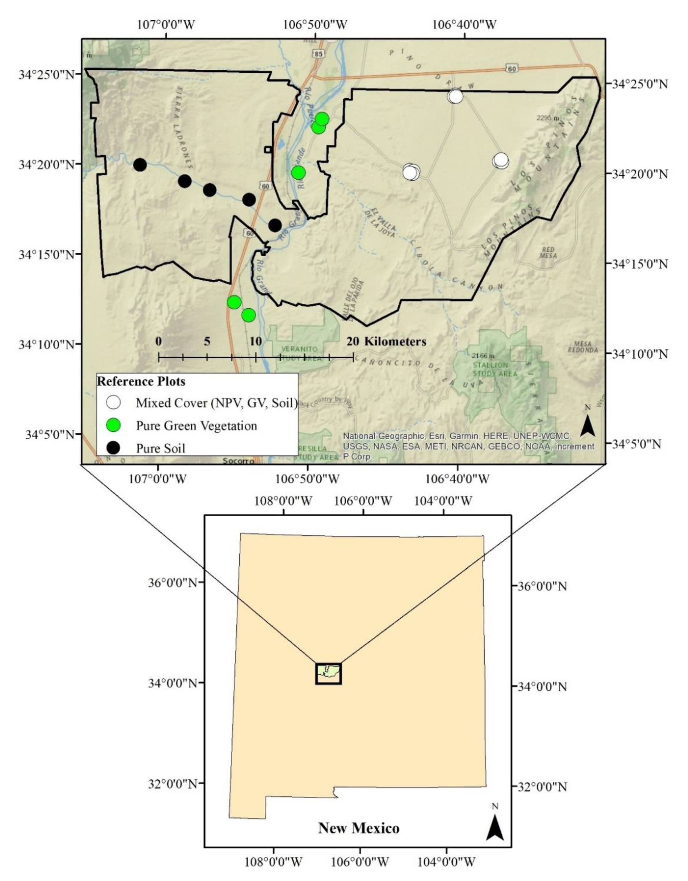
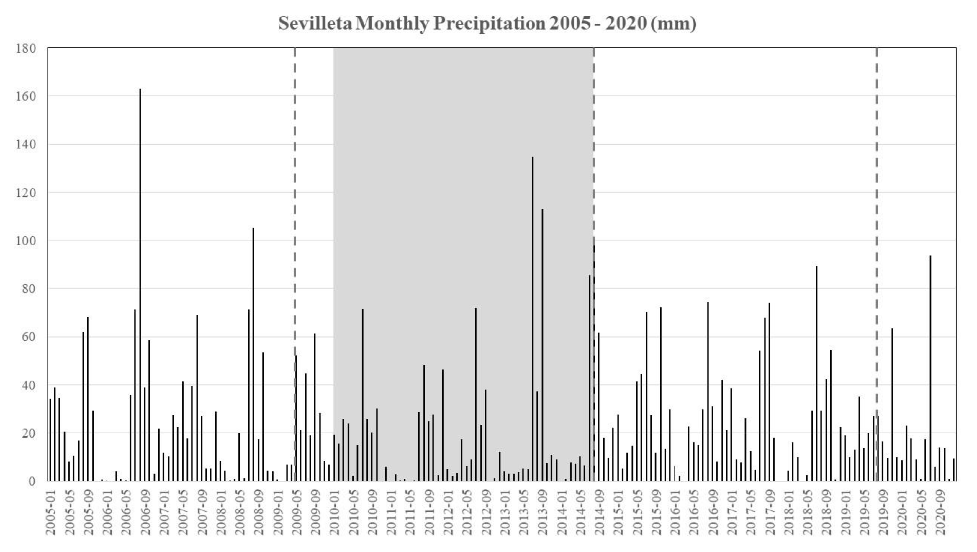
2.1. Study Site

The Sevilleta National Wildlife Refuge (SNWR), located in central New Mexico about 80 km south of the city of Albuquerque (Figure 1), is largely composed of former cattle rangeland which received refuge status in 1973 [20]. The refuge encompasses four biomes transitioning between Great Plains shortgrass prairie, Colorado Plateau shrub steppe, Chihuahuan desert, and pinon-juniper woodland [21]. The three main vegetation community types present on the refuge are blue grama (Bouteloua gracilis) grassland, black grama (Bouteloua eriopoda) grassland, and creosote (Larrea tridentata) shrubland; all are common dominant vegetation communities throughout the western US [21]. Smaller areas of the refuge include Rio Grande riparian woodland [21]. The refuge is home to a long-term ecological research station in the National Science Foundation’s LTER network that has been collecting data since 1988 [21]. Average elevation at the SNWR is ~1500 m [21].

The climate of the SNWR is semiarid, with average annual precipitation between 1981–2016 of 286 mm (±58 mm standard deviation), with relatively high interannual variability [22]. Precipitation comes in two phases: a brief summer monsoon pulse beginning between July and September, and winter precipitation from January to March. Grass and forb species tend to experience rapid growth patterns during the monsoon pulse, while shrub species tend to experience slower, steadier growth in the spring during snowmelt [23]. The average summer temperature is 24 °C; winter 5 °C [21]. The area experienced a brief and intense drought from 2010–2014 (Figure 2). While total annual rainfall was average in 2013, it occurred off the normal monsoon season, leading to persistence of severe drought conditions in 2014 in large portions of the state, including the SNWR [24].

2.2. Data

Field spectroscopy of dominant vegetation species were collected at the study area and post-processed to form a spectral library. The spectral library was used to unmix Landsat 5 TM imagery from 2009 and Landsat 8 OLI imagery from 2014 and 2019 with MESMA. Visible range high resolution imagery, collected using an uninhabited aerial system (UAS), was used to validate fraction estimates.

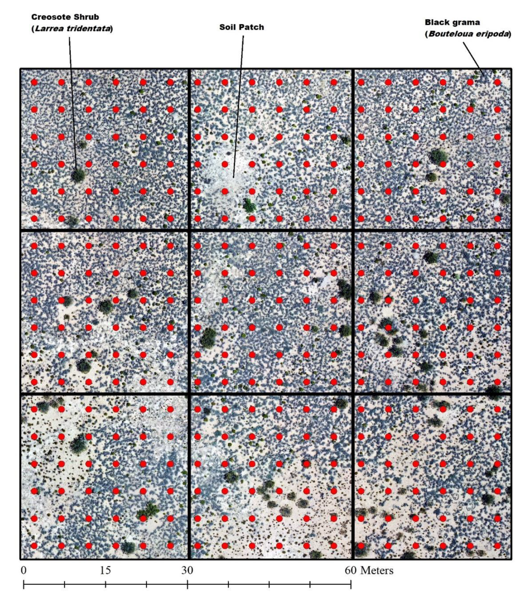
2.2.1. Field Spectroscopy

Spectral reflectance measurements of vegetation were collected monthly from May to September 2019 to build a comprehensive spectral library capturing dormancy and growth phases of the dominant grass and shrub species. An ASD Fieldspec 4 Standard Resolution Spectroradiometer with spectral range 350–2400 nm collecting 2151 bands (1.4 nm full width at half maximum from 350–1000 nm, 1.1 nm in width from 1001–2500 nm) was used to collect 10 measurements of each target in one burst. A Halon white reference panel was used to calibrate the equipment; a new white reference measurement was taken every 10 min during sampling. All measurements were conducted within +/− 2 h of solar noon, under cloud-free skies.

Four sampling sites were identified to capture the major vegetation community types at the refuge studied by the LTER: one black grama-dominated site, one creosote-dominated site, one blue grama-dominated site, and one mixed grass and shrub site. A minimum of 10 individuals of each major vegetation species at each site were sampled (

Table 1. Vegetation species sampled at the SNWR

USDA Species Code	Scientific Name	Common Name	No. Targets
BOGR2	Bouteloua gracilis	Blue grama	20
BOER4	Bouteloua eripoda	Black grama	31
LATR2	Larrea tridentata	Creosotebush	35
ATCA2	Atriplex canescens	Fourwing saltbush	14
CYIM2	Cylindropuntia imbricata	Tree cholla	20
EPTO	Ephedra torreyana	Torrey’s jointfir	22
GUSA2	Gutierrezia sarothrae	Broom snakeweed	29
JUMO	Juniperus monosperma	Oneseed juniper	8
CERCO	Cercocarpus montanus	Mountain mahogany	10
KRLA2	Krascheninnikovia lanata	Winterfat	9
OPUNT	Opuntia spp	Pricklypear	22
PRGL2	Prosopis glandulosa	Honey mesquite	4
YUGL	Yucca glauca	Soapflower yucca	15
DAPU7	Dasyochloa pulchella	Low woolygrass	2
PLJA	Pleuraphis jamesii	James’ galleta	7
SCBR2	Scleropogon brevifolius	Burrograss	4
SPORO	Sporobolus spp	Dropseed	3
CHER2	Chaetopappa ericoides	Rose heath	15
MAPIP	Machaeranthera pinnatifida	Lacy tansyaster	10

), though a few species that were rare at the landscape level but locally prevalent were also sampled opportunistically. At least one patch of bare soil with a minimum 60 cm diameter to avoid overhanging vegetation was sampled at each site. A total of 296 targets were sampled over six field dates.

Field spectra were individually examined in ViewSpecPro post-processing software. Obvious outliers and errors were discarded, referencing datasheet notes (e.g., clouds passed over during collection, disturbance to equipment, etc.): 20 target samples (i.e., 10 measurements of one target) were removed in this manner. The remaining spectra were then averaged by target and exported, resulting in 276 spectra.

2.2.2. Imagery Collection and Pre-Processing

Atmospherically corrected imagery with <5% cloud cover was acquired from the Landsat Ecosystem Disturbance Adaptive Processing System (LEDAPS). Landsat TM and Landsat OLI scenes were selected to track vegetation dynamics from five years pre-drought (2009), peak drought (2014), and five years post-drought (2019). Image dates were filtered to correspond as closely as possible to mid-May, the optimal spectral separability season between NPV, GV, and S in a nearby study area [17], as well as the anniversary date of UAS reference imagery collection (26 June 2019). Three scenes from Path 33 Row 36 were selected with image dates 10 May, 2009; 9 June, 2014; and 30 June, 2019 (Figure 2).

High resolution airborne imagery was collected at three sample sites on 26 June, 2019 using a DJI Mavic Pro UAS equipped with a Hasselblad L1D-20c sensor (Figure 1). Flights were conducted at 120 m AGL with 80% forelap and 60% sidelap between frames, with a GSD of ~2.5 cm; altogether, 323 frames were collected across all sites (129 at site 1, 76 at site 2, and 118 at site 3). Two sites were located near previously established LTER vegetation monitoring sites: one near the creosote shrubland and black grama grassland monitoring sites, and the other near the blue grama grassland monitoring site. The last sampling site was located in the blue and black grama grassland ecotone. Each site covered at least 2.5 km². To facilitate accuracy assessment of the 2019 endmember fraction images, orthomosaics with 2.5 cm spatial resolution and estimated positional accuracy +/− 3 m were produced from the imagery using Agisoft Metashape Professional photogrammetry software.

2.2.3. Vegetation Community Map

A vegetation community classification map for the SNWR [25] was retrieved from the Sevilleta LTER database to examine changes in NPV, GV, and S by vegetation community type.

2.3. Analysis

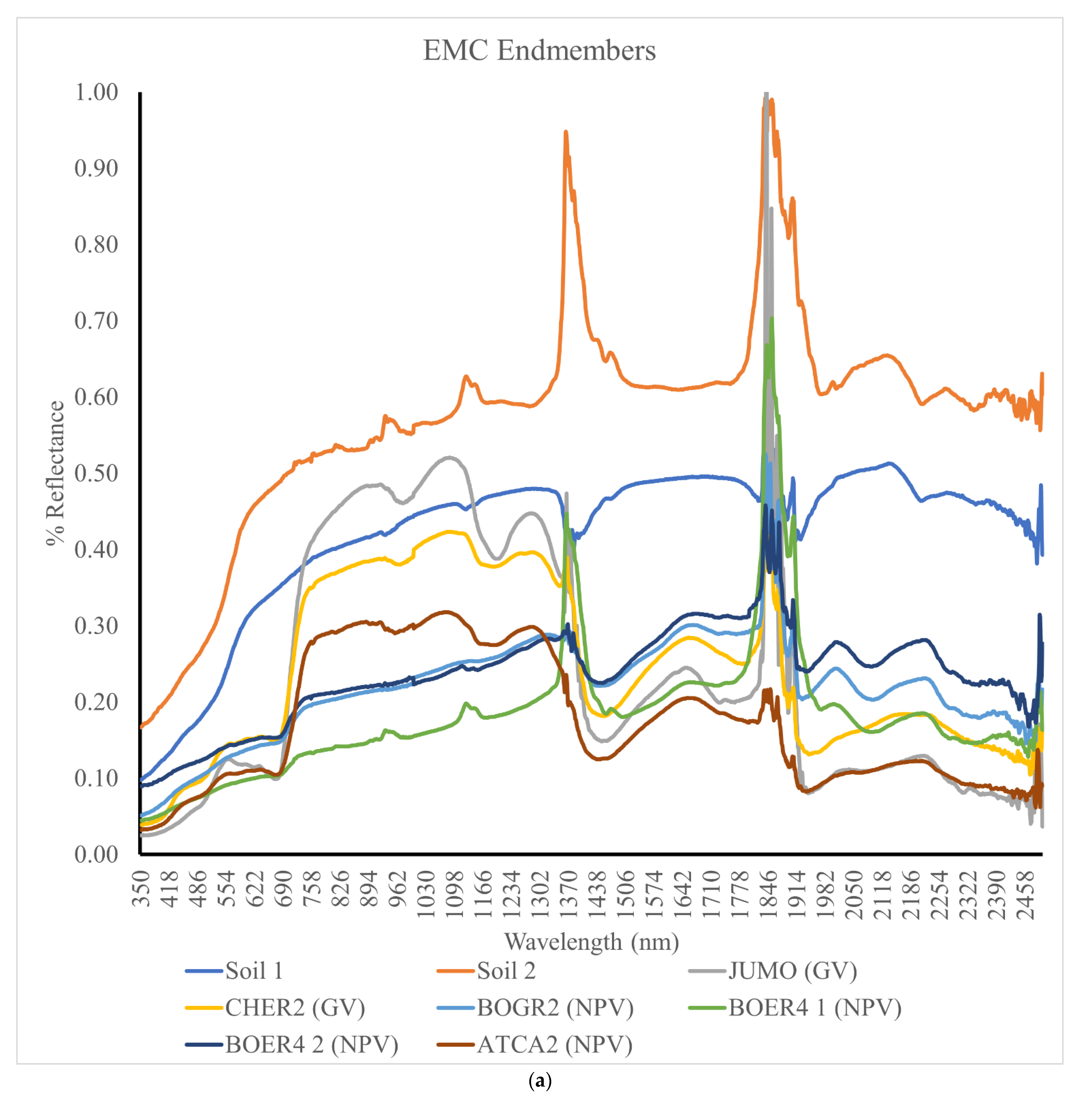
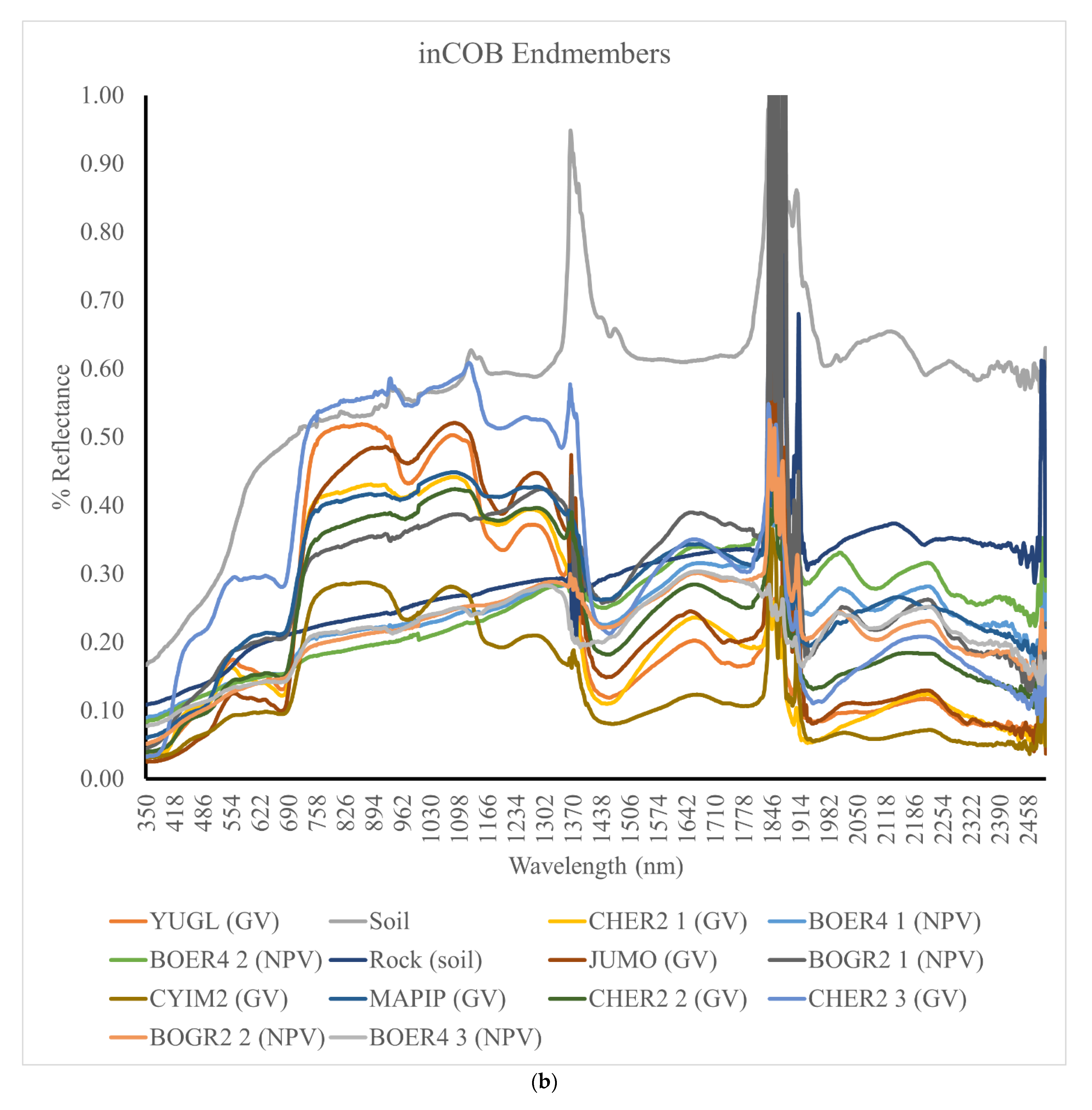
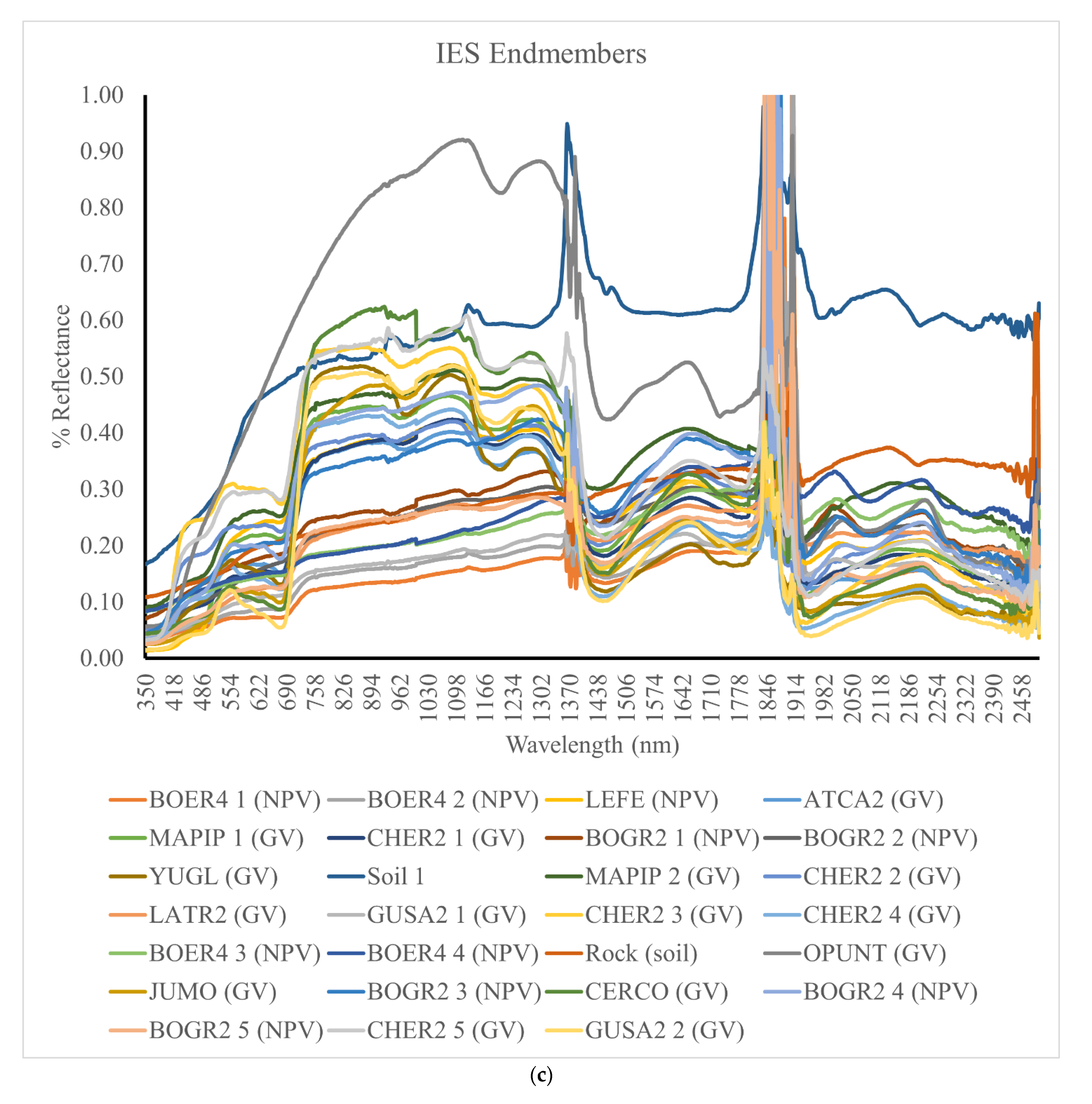
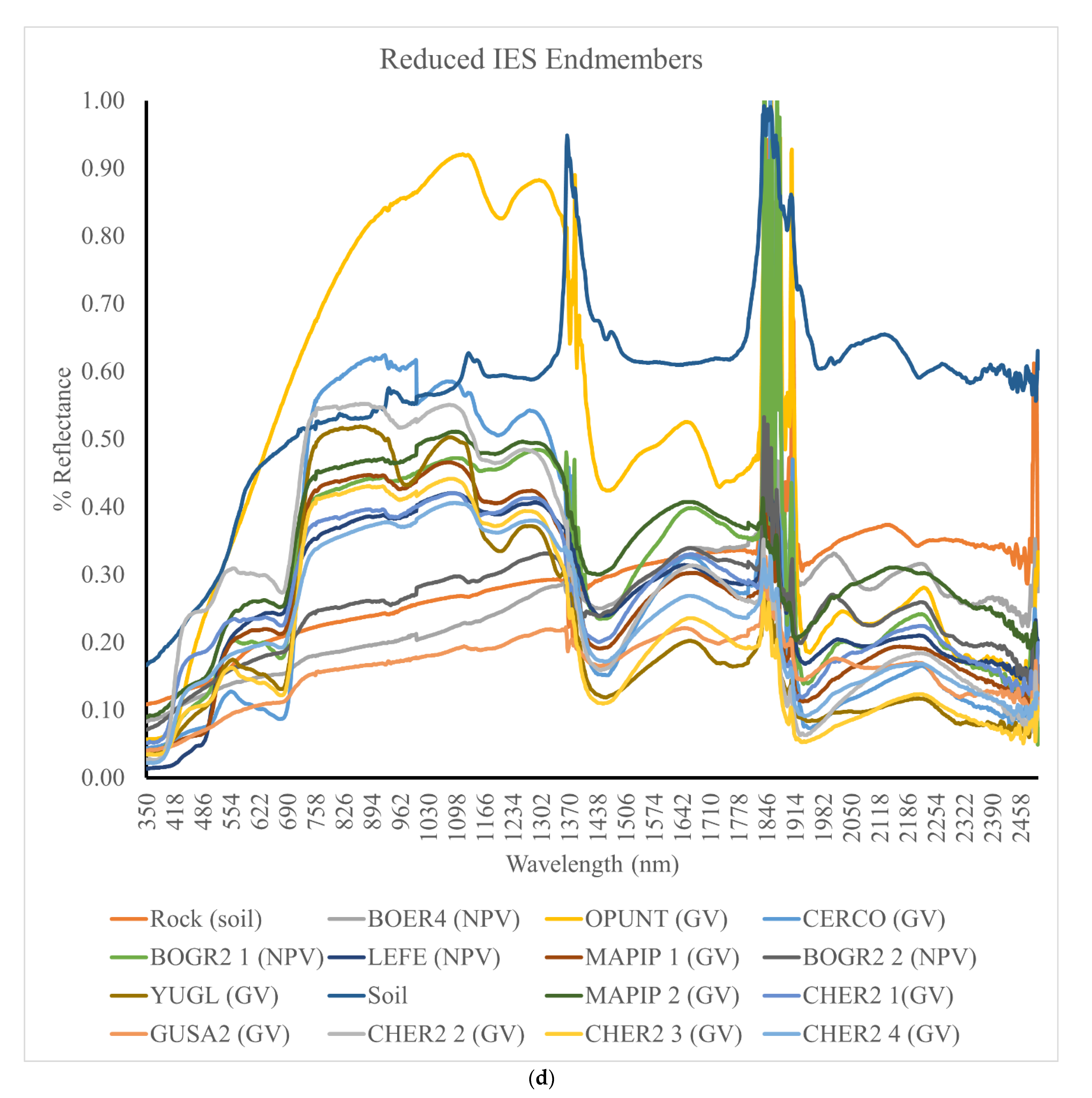
2.3.1. Spectral Library Creation and Optimization

A spectral library was constructed from the combined field-collected spectra from all dates using the open-source Visualization and Image Processing for Environmental Research (VIPER) 2.1 toolset [26] in ENVI 5.2. The field spectra were convolved to Landsat 8 OLI and Landsat 5 TM bands, creating two master libraries of the same set of spectra. Bands 2–7 were then reserved from the OLI library and bands 1–5 and 7 were reserved from the TM library to align the spectral coverage of the two sensors. The spectral separability of NPV, GV, and S were evaluated using Jeffries-Matusita distance prior to analysis; each individual pair comparison scored 1.93 or above (GV-NPV: 1.94; NPV-S: 1.99; GV-S: 1.99), with the maximum possible score of 2 [27]. These scores are considered highly separable for classification purposes [28].

Four endmember selection methods, outlined below, were used to derive optimized libraries for the MESMA (

Table 2. Results of four endmember (EM) selection methods on spectral library composition

Endmember Selection Method	Citation	No. NPV EM	No. GV EM	No. S EM
EMC	Tane et al., 2018	3	3	2
inCOB	Roberts et al., 2003	4	8	2
IES	Roth et al., 2012	5	21	2
Reduced IES	Roth et al., 2012	3	11	2

). Spectral reflectance curves of selected endmembers in each optimized library can be viewed in Appendix A.

There are three main metrics for evaluating potential endmembers based on spectral characteristics: count-based endmember selection (CoB), endmember average RMSE (EAR), and minimum average spectral angle (MASA). The three together are referred to as EMC (EAR/MASA/CoB) metrics.

The first two metrics, EAR and MASA, are similar to each other in that they evaluate intraclass variability; minimizing both values selects the endmembers that best model other members of the same class. EAR and MASA use the same formula, but MASA evaluates summed spectral angle in place of RMSE to determine the endmember that best models others of the same class [29].

Count-based endmember selection (CoB) is another metric to select the endmembers that best model others within the same class [30]. MESMA is applied to the spectral library instead of the image, yielding two values: the number of spectra within the class modeled by a given endmember (inCoB), and the number of spectra outside of the class modeled by a given endmember (outCoB). An ideal endmember will have an inCoB equal to the number of spectra in the same class, with outCoB equal to zero [26].

Multiple methods have been developed for endmember selection based on some combination of EMC metrics. For this study, two methods were used to derive two separate libraries. The first library (‘EMC’) selected three endmembers per class (NPV/GV/S): the single spectra with the lowest EAR, the lowest MASA, and the highest inCoB, respectively. In cases where the same individual endmember was selected through multiple metrics (for example, if the same spectra had both the lowest EAR and highest inCoB), fewer endmembers were selected for that class. This method was validated by Tane and colleagues [29] in their comparison of endmember selection methods and has the benefit of taking advantage of all metrics for selecting the spectra maximally representative of in-class variability. The resulting EMC library contained 8 endmembers: 3 NPV, 3 GV, and 2 S.

The second library (‘inCoB’) filtered only by inCoB value; all unique inCoB values >0 were reserved. EAR and MASA were considered only to break ties between spectra with the same inCoB value. This method was validated by Roberts and colleagues [30] in a study of a semiarid shrubland system in California. This method ensures that all selected endmembers can be used to model others of the same class, a factor not guaranteed by favorable EAR or MASA values. The inCOB library contained 14 endmembers: 4 NPV, 8 GV, 2 S.

Two iterative endmember selection (IES) techniques were also tested. IES maximizes class separability by selecting potential endmembers with the highest kappa values for modeling the entire library [31]. Two libraries were created using IES as an optimization method- an ‘original’ IES and a ‘reduced’ IES library. The original IES (IES) used only a single pass of the algorithm, while the reduced IES library used a fresh pass on each derived library, until the derived library no longer reduced with a new pass. The advantage to reduced IES over single-pass IES is savings in computational power by reducing the number of endmembers in the library [32]. The IES library contained 28 endmembers (5 NPV, 21 GV, and 2 S), while the reduced IES library contained 16 (3 NPV, 11 GV, and 2 S).

2.3.2. Multiple Endmember Spectral Mixture Analysis

Landsat pixels were unmixed by modeling fractional cover of green (photosynthetic) vegetation (GV), non-photosynthetic vegetation (NPV), soil (S), and photometric shade. The four libraries were each used to unmix Landsat imagery from 30 June 2019.

Three parameters were altered on each run to improve model accuracy. Adjustments were made to the overall RMSE threshold, the multifusion threshold, and the use of stable zone unmixing. First, the overall model RMSE threshold, below which a pixel remains unmodeled, was set at either 0.025 or 0.007, the former being standard in the literature [14] and the latter adjusted to match the accepted optimum setting for the multifusion threshold.

The multifusion threshold, which is the RMSE at which the algorithm switches from a model with fewer endmembers to more endmembers, was set at either 0.025 or 0.007. Adjusting this value lower should make the model more likely to select more endmembers to model a pixel in complex environments; this is potentially useful in an environment like the SNWR, where variability of cover is high at fine spatial scales, and all cover types are expected to be present within most pixels. Roberts et al. [32] found the optimum setting to be 0.7% after testing in multiple complex environments; a threshold of 2.5% was also tested to correspond to the overall RMSE threshold.

Finally, stable zone unmixing, which subsets the bands in an image set for analysis by preserving only those which maximize separability of each endmember pair [33], was tested for each threshold configuration.

With all parameter adjustments combined, each library was used to unmix the Landsat image eight times, yielding 32 MESMA runs in total (see Appendix A). For all runs, the range of possible endmember fractions was constrained from –0.05 to 1.05, consistent with the literature for this environment [17], and the maximum shade fraction was constrained to 30% to prevent over-modeling of shade in the largely barren and open study area. Only three- and four-endmember models were enabled due to the high variability of cover over small spatial scales in the study area noted in the mixed reference plots (

Table 3. Cover fractions of NPV, GV, and soil for all reference plots. Some rows may not sum to 100% due to rounding.

Plot ID	NPV Fraction	GV Fraction	Soil Fraction	Community Type	Imagery Source
Green 1–5	0%	100%	0%	Agriculture	Landsat / NAIP
Soil 1–5	0%	0%	100%	Barren (Arroyo/Wash)	Landsat / NAIP
BOER4_1	45%	13%	43%	Grassland	UAS
BOER4_2	55%	5%	40%	Grassland	UAS
LATR2_1	15%	32%	53%	Shrubland	UAS
LATR2_2	38%	16%	46%	Shrubland	UAS
LATR2_3	39%	15%	46%	Shrubland	UAS
LATR2_4	32%	21%	46%	Shrubland	UAS
BOGR2_1	71%	2%	27%	Grassland	UAS
BOGR2_2	51%	10%	40%	Grassland	UAS
BOGR2_3	62%	2%	36%	Grassland	UAS
Transition 1	35%	9%	56%	Grassland	UAS
Transition 2	44%	11%	45%	Grassland	UAS
Transition 3	42%	9%	48%	Grassland	UAS

), creating the expectation that all cover types would be present in a majority of pixels. All models were shade-normalized prior to accuracy assessment.

Accuracy assessment was performed to determine which MESMA-derived fraction images best modeled all three classes of cover in 2019. The library and settings for the run that derived the best fit 2019 fraction image were used to unmix imagery from 2009 and 2014. Because suitable reference imagery was not available, independent accuracy assessment was not performed for the 2009 and 2014 fraction images.

2.3.3. Accuracy Assessment

Two types of reference plots were used to evaluate the fit of the models: plots of pure green vegetation or soil; and mixed plots of NPV, GV, and soil (Table 3). To derive the mixed plots, 90 × 90 m grids representing the ground footprint of nine Landsat pixels were overlaid on the UAS reference imagery. The size of the plots was set to allow for minor co-registration errors between the Landsat and reference imagery. Three plots were randomly selected from each reference imagery collection site, plus two more at the creosote collection site to allow for a more representative balance between grass- and shrubland, to yield 12 mixed plots (Figure 1, Table 3). The plots were overlaid with a dot matrix of 18 by 18 points, or 324 points per plot (Figure 3). The cover type beneath each point was classified through manual interpretation to yield estimates of fractional cover of NPV, GV, and S for each plot. A least-squares regression analysis was then used to compare the fractional cover between the reference and MESMA-estimated cover fractions [17,34].

Pure cover plots were derived from the 2019 Landsat 8 imagery displayed in a false color composite (bands 7, 5, and 2) to emphasize soil through the SWIR band and vegetation through the NIR band. Five plots of 100% soil cover were identified in arroyos and other natural drainages based on red saturation (the higher the saturation, the drier/likely purer soil, lack of vegetation). Five plots of 100% green vegetation cover were derived from agricultural areas based on green saturation (the greener the saturation, the more densely vegetated). National Agriculture Imagery Program (NAIP) imagery from 2014 was used to verify the accuracy of these interpretations. We were unable to locate unmixed areas of non-photosynthetic vegetation of sufficient size in the study area; even in grassland environments, there was only one plot where NPV cover exceeded 60% (Table 3). The same least-squares regression was used to compare fractional cover estimates between the pure reference plots and the MESMA-estimated cover fractions. RMSE, mean average error (MAE), and R² values were derived for each of the three cover classes in both types of reference plots.

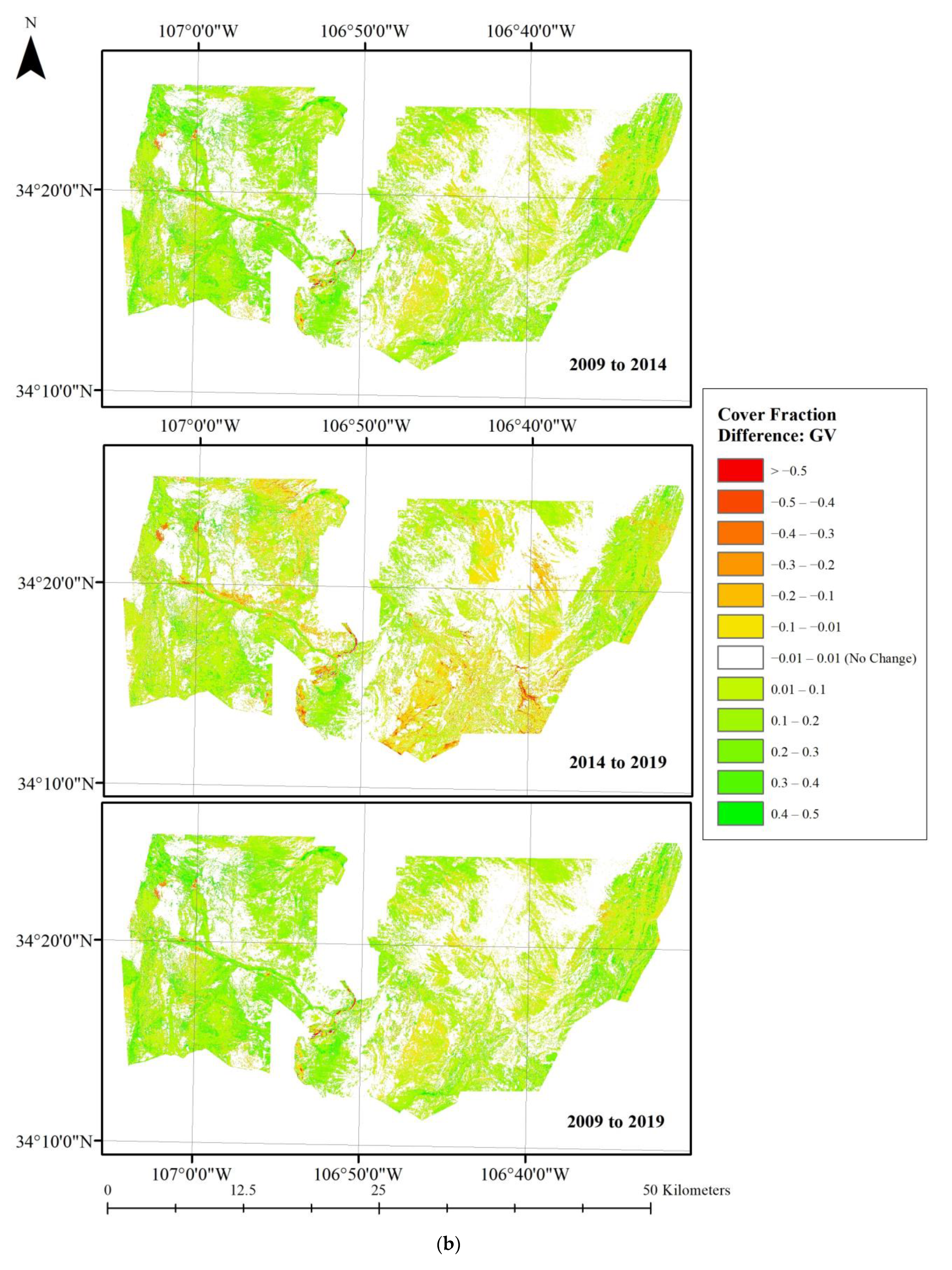
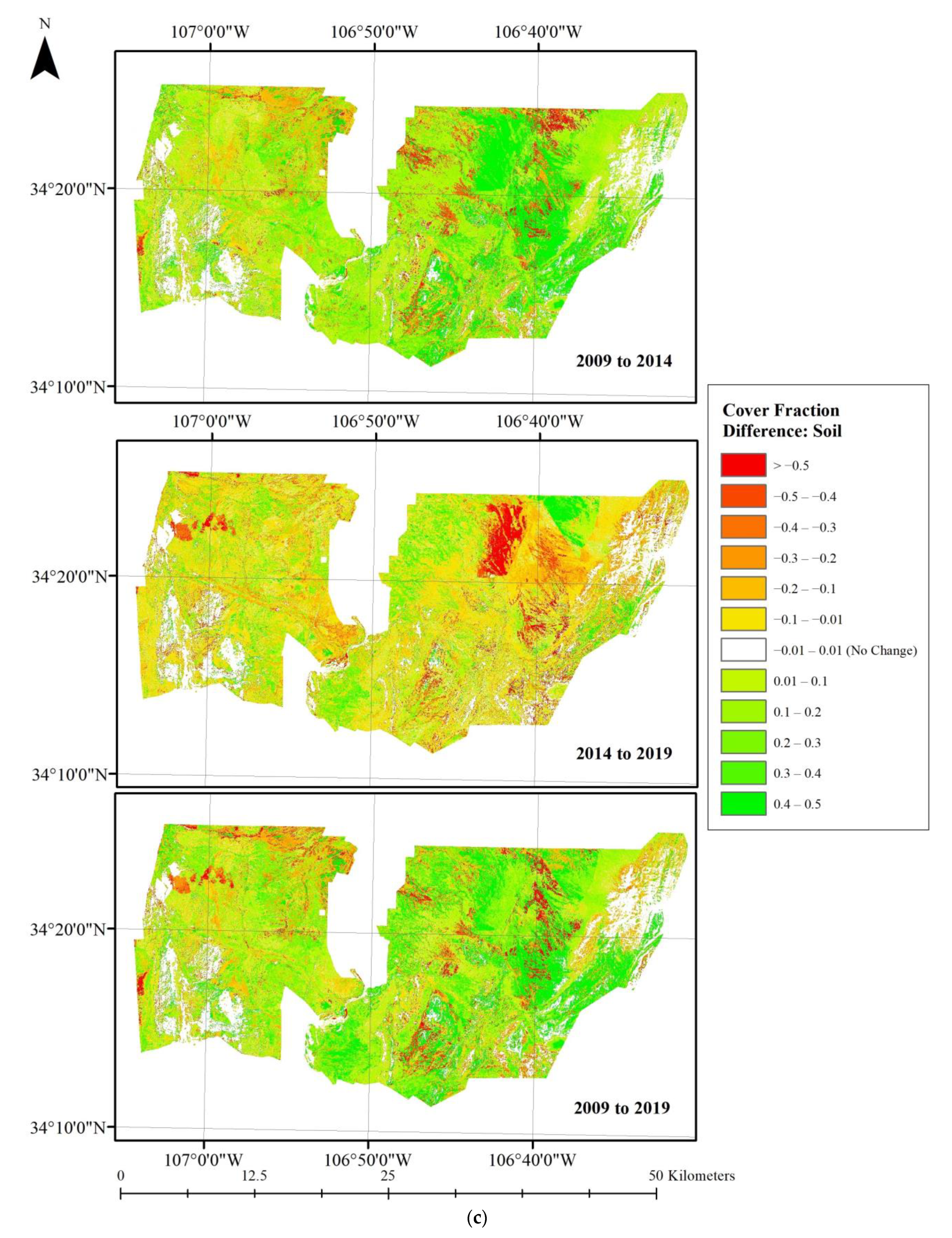
2.3.4. Changes in Fractional Cover by Vegetation Community

Fraction images from 2009, 2014, and 2019 were differenced in the following combinations: 2009/2014; 2014/2019; and 2009/2019. The differenced images were overlaid with a vegetation community classification map from a prior LTER study [25] and zonal statistics were calculated to evaluate changes in NPV, GV, and soil over the study period in black grama grassland, blue grama grassland, the grassland ecotone between the two, and creosote shrubland. These community types collectively form ~35% of total cover on the SNWR, and ~57% of cover on the east side of the refuge, where long-term research sites are located.

3. Results

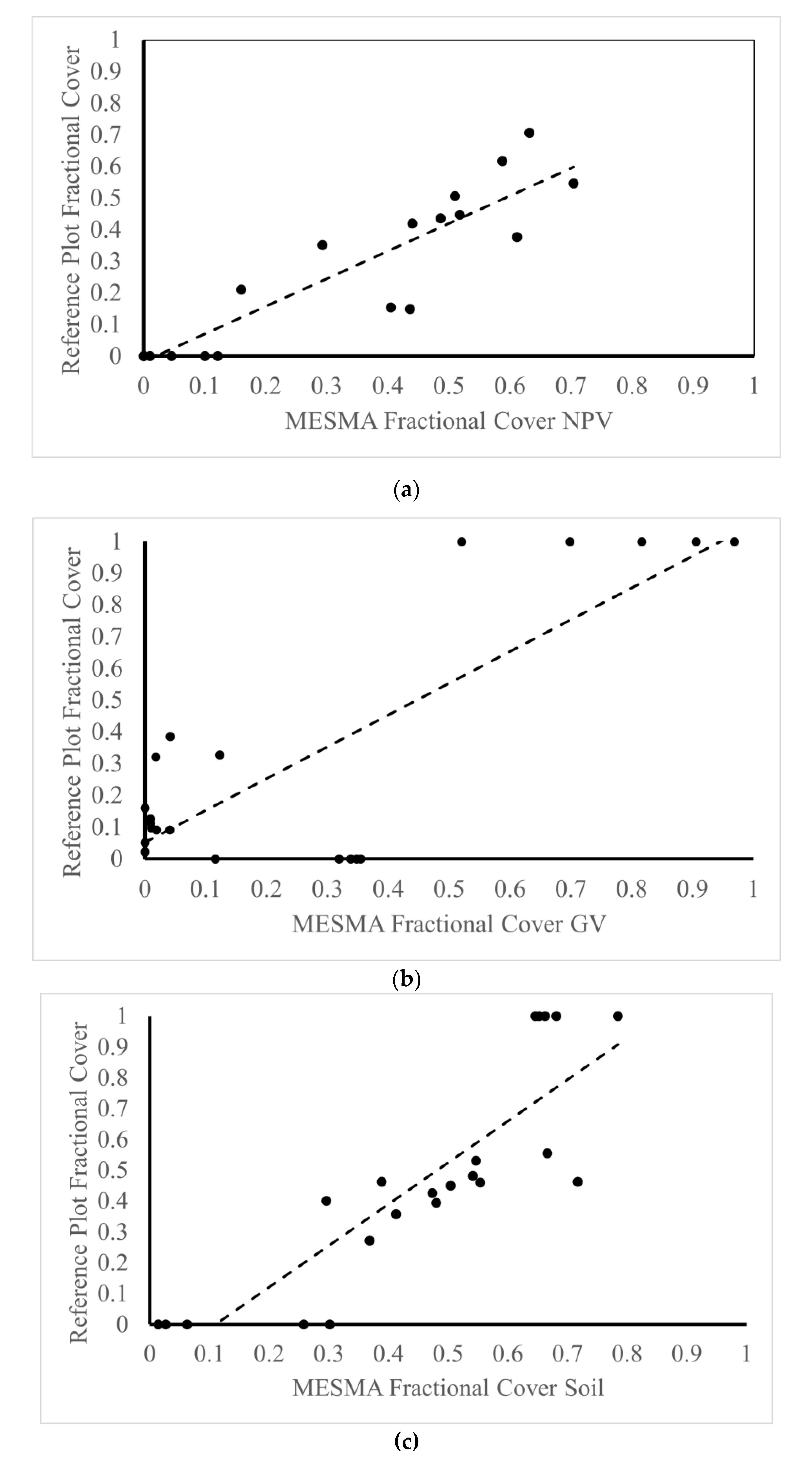
3.1. Accuracy Assessment

The best fit model was derived from the MESMA using an EMC library with RMSE and multifusion threshold set to 0.025 with no stable zone unmixing (Figure 4). The class with the lowest level of agreement was GV, with an R² of 0.67 and the highest RMSE and MAE of all classes. The class with the highest level of agreement was NPV, with the lowest RMSE and MAE of all classes, and an R² of 0.85. Soil also showed agreement, with an R² of 0.74, though with slightly higher RMSE and MAE than NPV. The library and metrics used to derive the best fit model for 2019 were used to unmix imagery for 2009 and 2014 to assess cover dynamics during and after the drought period.

While some of the other fraction images showed higher agreement modeling individual classes, particularly soil, none of the rest successfully modeled all three. 55% (n = 20) of models failed to model a sufficient number of pixels to perform an accuracy assessment, largely driven by the inCoB library failing to produce a single assessable model (see Appendix A). Of the models for which accuracy assessment was possible, both the IES and Reduced IES libraries failed to model NPV and GV, with R² values never exceeding 0.41 and often <0.1 (see Appendix A). Only one other EMC library produced a model with R² > 0.7 for any class: the EMC with RMSE of 0.025 and multifusion of 0.007 had higher agreement for soil, with R² of 0.74.

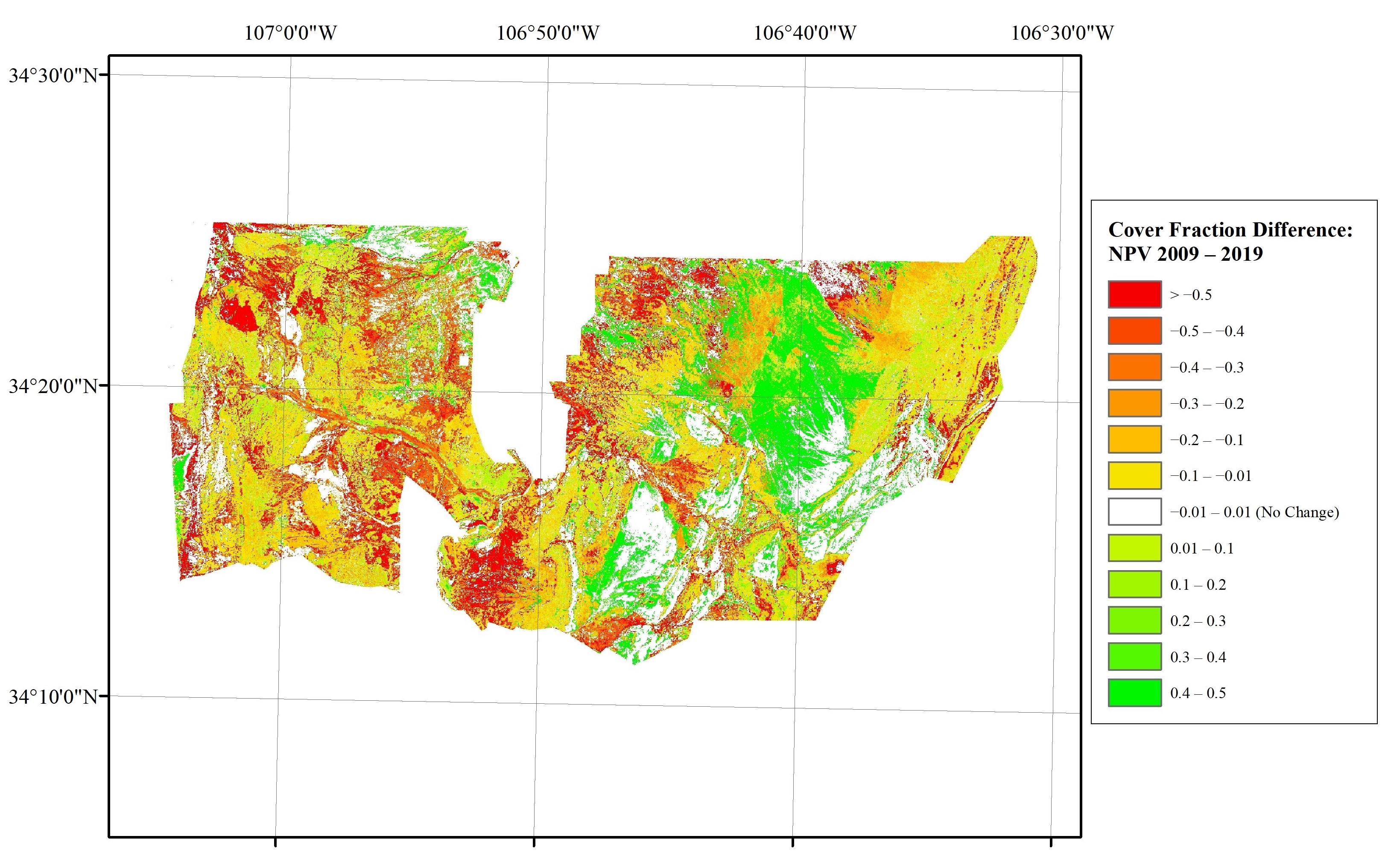
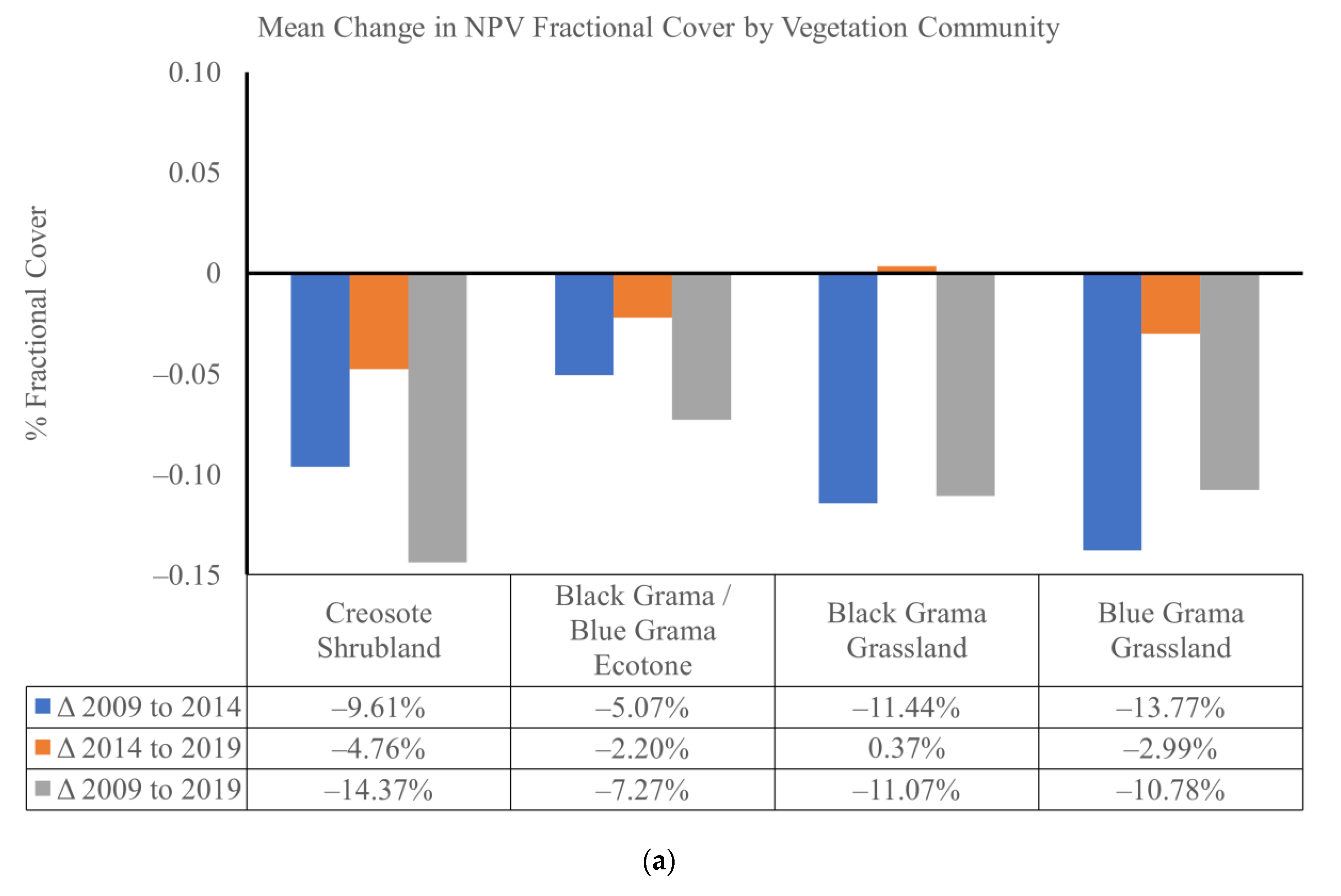
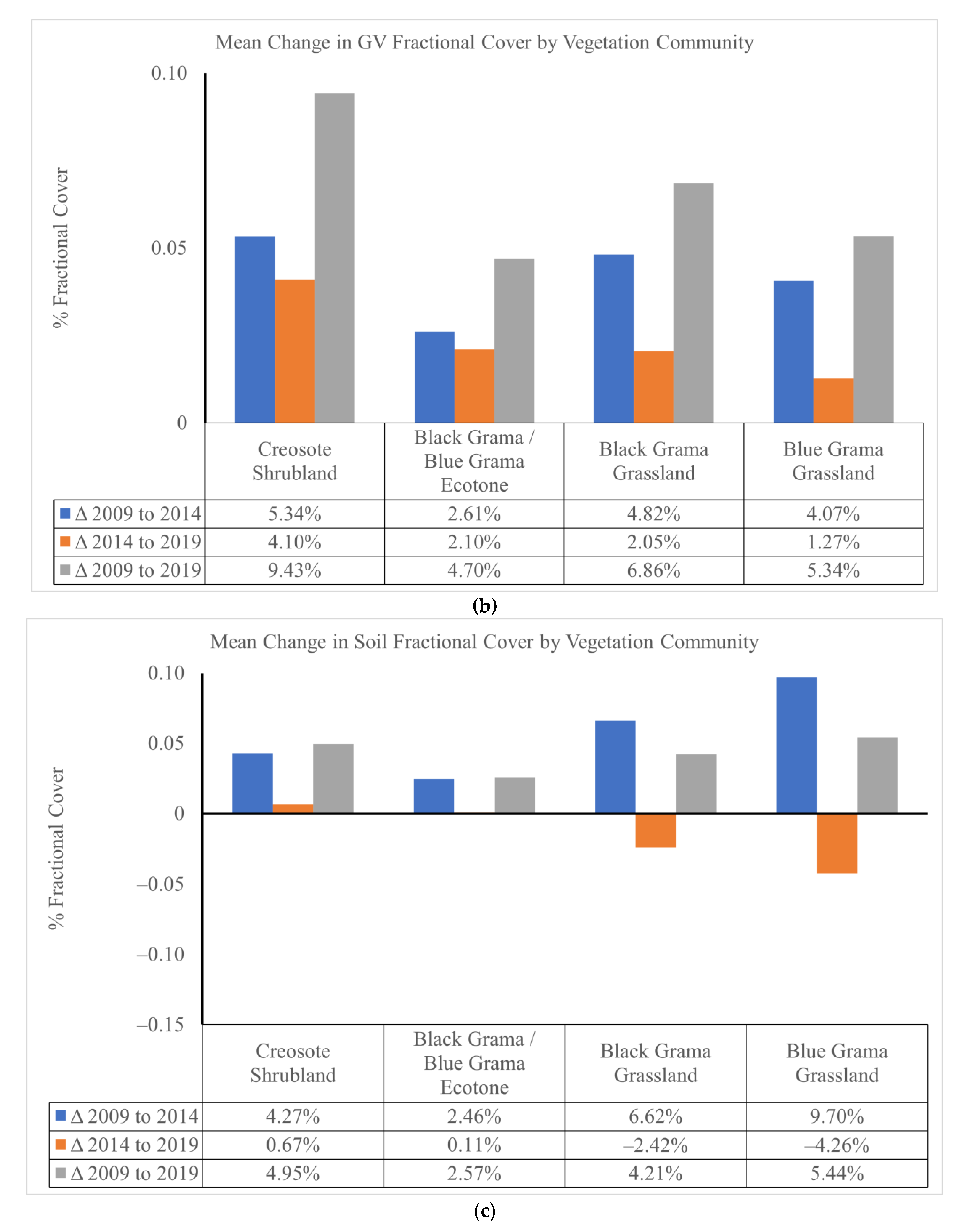
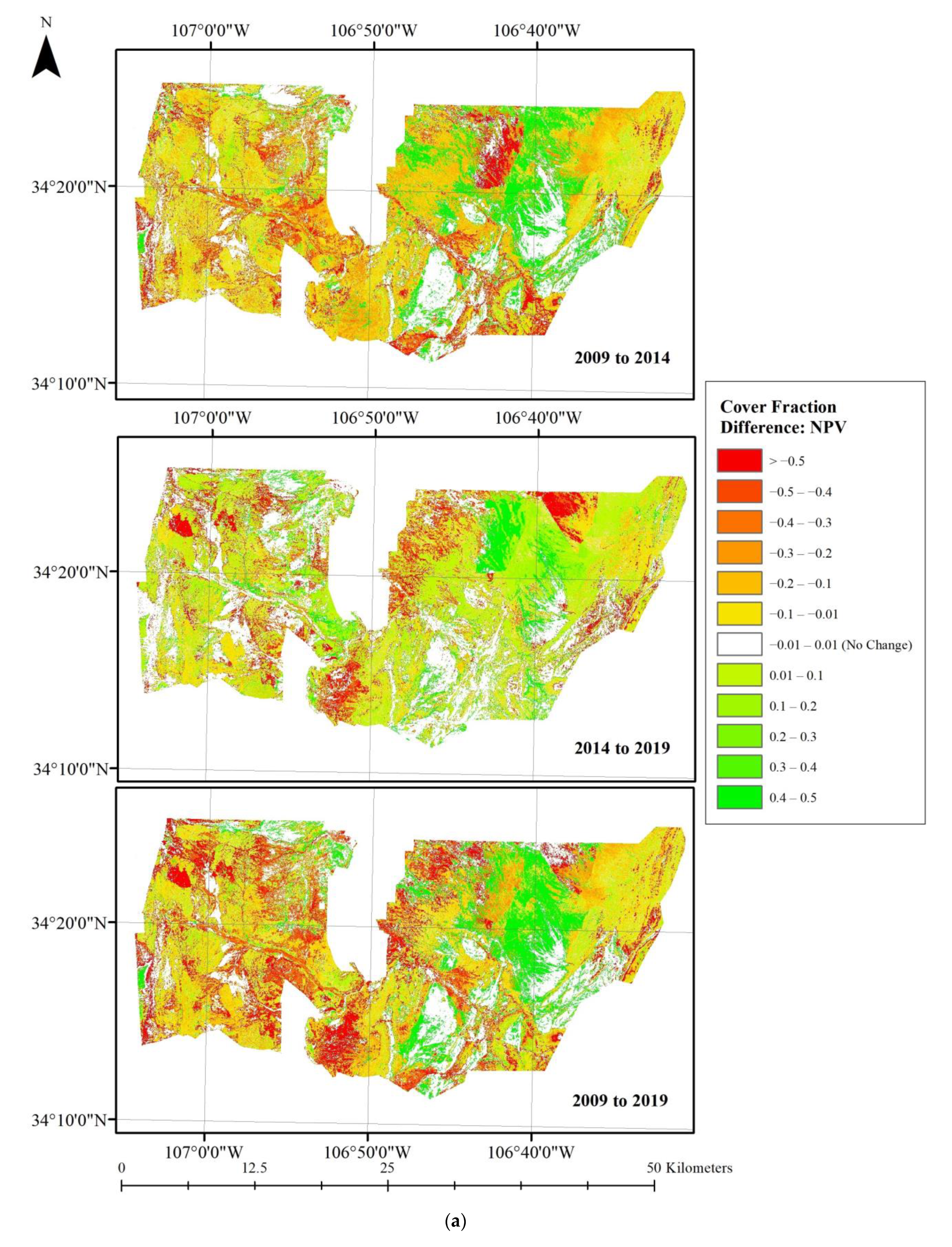
3.2. Changes in Fractional Cover by Vegetation Community

Changes in fractional cover were evaluated for the drought period (2009–2014) and the post-drought period (2014–2019) for each cover type (Figure 5). The general trends captured on the landscape scale by the differenced images show a pattern of vegetation loss during the drought period, as evidenced by the general increases in soil fraction accompanied by declines in NPV (Figure 6). The differenced images do not indicate an overall return to the pre-drought baseline, which is underlined when the change over time is examined by community type (Figure 5).

Non-photosynthetic vegetation fractions declined in all community types during the drought period. Blue grama grassland had the steepest drought period decline, at 13%, followed by black grama grassland at 11% and creosote shrubland at 9%. The ecotone experienced the smallest decline, at 5%, perhaps due to species diversity enhancing drought resilience [35]. In the post-drought period, NPV fractions continued to decline in creosote shrubland and in the ecotone, at 4% and 2% respectively. Blue grama grassland experienced modest recovery during the post-drought period, at 2%, which was not sufficient to return to baseline cover. There was virtually no change in NPV fraction in black grama grassland.

Green vegetation fractions increased in all community types over the study period, including during the drought period. The largest increase was in creosote shrubland, with a 5% increase during the drought period and a continued 4% increase during the post-drought period—a total 9% increase over the study period. Black and blue grama grassland both experienced increases of 4–5% during the drought period and an increase of 1–2% during the post-drought period. The ecotone experienced a slightly smaller increase, with 2% during the drought period and 2% during the post-drought period.

Soil fractions increased in all community types over the course of the total study period (2009–2019), with virtually all increases occurring during the drought period. The steepest drought period increase, 9%, occurred in the blue grama grassland. Black grama grassland soil fraction increased by 6%, creosote shrubland by 4%, and the ecotone by 2%. The black grama grassland and the blue grama grassland both experienced slight declines in soil fraction during the post-drought period of 2% and 4% respectively, which was not sufficient to return to the pre-drought baseline. There was virtually no change in soil fraction in the post-drought period in the ecotone or creosote shrubland.

4. Discussion

Only one MESMA run, using EMC endmember selection and RMSE and multifusion thresholds of 0.025, produced a fraction image that successfully modeled fractional cover in 2019. The IES and CoB libraries likely failed due to phenological mismatches between these libraries and the Landsat imagery. Because CoB weights the spectra that capture the highest amount of variability within a class, spectra that modeled the full range of phenological variation from May through September may not have been appropriate for modeling vegetation spectra in June specifically. IES weights endmembers that best model an entire library; similarly, the spectra that best modeled the library as a whole may have captured inappropriate spectral variations for modeling vegetation spectra in June.

The interventions in thresholding and stable zone unmixing generally did not provide appreciable increases in model accuracy. Stable zone unmixing is more likely to improve results for image sets with high spectral resolution [33]; the Landsat scenes, after adjustments to the layer stacks to align the spectral coverage of OLI 8 and TM5, left only six bands for analysis. Adjustments to the RMSE and multifusion thresholds gave similar results in terms of percentage of pixels modeled and overall accuracy in different runs derived from the same library. However, adjusting the multifusion threshold to 0.025 to match the overall RMSE threshold boosted accuracy for GV for the best fit model. It is known that lower multifusion thresholds favor the selection of models with more endmembers [32].

The most dramatic change in all community types was the decrease in NPV fraction, with declines of roughly 10% in most communities, which is consistent with expectations of grassland dieback during drought. The increases in GV across community types in the drought and post-drought period are consistent with observations of community reordering occurring under climate change in semiarid grasslands [6]. A study of drought legacy effects on aboveground net primary production (ANPP) additionally found an increase in ANPP at two SNWR sites when rainfall increased in the study area in 2013 [36], despite the continued regional drought pattern, which may account for some of the GV increase observed in these results. The blue grama grassland was the only community to experience recovery in NPV fraction in the post-drought period. This observation, combined with the similar declines in NPV fraction between black grama and blue grama grassland, contradicts observations of black grama grassland’s greater resilience in drought [37]. However, the change in GV should be viewed with some caution given the RMSE of the best fit model for green vegetation exceeded the percent change in cover observed (see Appendix A).

There were notable limitations to the best fit 2019 model, the foremost of which was its unreliability at detecting green vegetation at less than ~30% cover (Figure 4), consistent with the literature for this environment [15], particularly given the limited spectral information from the imagery set analyzed [38]. Multiple climatic and physiological factors likely contributed to this issue. First, GV was likely a weak signal due to the comparatively low presence of green vegetation throughout the grassland and shrubland in study area: in the mixed reference plots, green vegetation averaged 12% cover and never exceeded 33%, even in shrubland. The already low concentrations of GV were likely limited in 2019 due to a weak monsoon pattern, leading to only a limited ‘green up’ of grasses at the SNWR and to some extent even perennial shrubs. The spectral similarity between non-photosynthetic vegetation and soil, and the weak spectral curve of ‘green’ desert grasses and shrubs, even in the best of conditions, may have also contributed to the difficulty in deriving an accurate model for GV [5].

Two methods might be used to address this shortcoming. The first, and most straightforward, is the use of an imagery set with more spectral information. The drawback is the limited availability of hyperspectral imagery for the area of interest and the comparatively short temporal record of this imagery hindering the ability to assess dynamics over long time periods, one of the main advantages of Landsat. MODIS, another multispectral image source with greater spectral coverage than Landsat, could present an alternative, but Okin [39] found that NPV and soil were not separable using MESMA on MODIS bands, and instead used a relative spectral mixture analysis (RSMA) to track changes in fractions relative to a specified time. RSMA would be useful for tracking landscape-level trends in changes in fractions of GV, NPV, and S, but would not be suitable for mapping as it does not attempt to quantify absolute cover [39]. Another method might be the introduction of multitemporal endmembers and the unmixing of multidate image stacks [33,40]. With phenological variation as an additional variable, it may be possible to emphasize even a relatively weak green signal [34].

Though no independent accuracy assessment was performed to confirm the reliability of the 2009 and 2014 fraction images, other multidate MESMA studies have successfully used the same field-spectra derived library to unmix imagery sets of the same area across time [17,34]. It is worth noting that the high interannual climatic variability of deserts leads to substantial changes in average spectral curves within classes, and spectral separability between classes [5], which could impact the reliability of results from year to year. Both the field spectra and the reference imagery in 2019 will allow future retrospective investigations to address this possible issue, given that both will be available to the public through the NSF LTER database.

5. Conclusions

We present a workflow to utilize MESMA to estimate cover fractions of GV, NPV, and S in semiarid grass- and shrubland with high accuracy using Landsat imagery as a base. The ability of MESMA to track NPV dynamics provides a more comprehensive representation of vegetation dynamics in semiarid systems over traditional vegetation indices such as NDVI due to these indices reliance on greenness, which is often ephemeral in these systems. The changes detected during and after the drought period indicate better understanding of NPV fraction will be critical to tracking vegetation dynamics in these systems, especially as drought events are expected to increase in frequency and intensity in this region [2,3]. Because of its ability to accurately model NPV fraction, MESMA is useful tool for tracking vegetation dynamics at the landscape scale in semiarid systems.

References

1. Masson-Delmotte, V.; Zhai, P.; Pirani, A.; Connors, S.L.; Péan, C.; Berger, S.; Caud, N.; Chen, Y.; Goldfarb, L.; Gomis, M.I.; et al. (Eds.) IPCC: Climate Change 2021: The Physical Science Basis. Contribution of Working Group I to the Sixth Assessment Report of the Intergovernmental Panel on Climate Change; Cambridge University Press: Cambridge, UK, 2021. [Google Scholar]
2. Williams, A.P.; Cook, E.R.; Smerdon, J.E.; Cook, B.I.; Abatzoglou, J.T.; Bolles, K.; Baek, S.H.; Badger, A.M.; Livneh, B. Large Contribution from Anthropogenic Warming to an Emerging North American Megadrought. Science 2020, 368, 314–318. [Google Scholar] [CrossRef]
3. Hurd, B.H.; Coonrod, J. Climate Change and Its Implications for New Mexico’s Water Resources and Economic Opportunities; Technical Report 45; New Mexico State University Agricultural Experiment Station: Las Cruces, NM, USA, 2008. [Google Scholar]
4. Knapp, A.K.; Carroll, C.J.W.; Denton, E.M.; La Pierre, K.J.; Collins, S.L.; Smith, M.D. Differential Sensitivity to Regional-Scale Drought in Six Central US Grasslands. Oecologia 2015, 177, 949–957. [Google Scholar] [CrossRef] [Green Version]
5. Okin, G.S.; Roberts, D.A. Remote Sensing in Arid Regions: Challenges and Opportunities. In Remote Sensing For Natural Resource Management and Environmental Monitoring: Manual of Remote Sensing, 1st ed.; Ustin, S.L., Ed.; John Wiley & Sons: New York, NY, USA, 2004; pp. 111–145. [Google Scholar]
6. Jones, S.K.; Ripplinger, J.; Collins, S.L. Species Reordering, Not Changes in Richness, Drives Long-Term Dynamics in Grassland Communities. Ecol. Lett. 2017, 20, 1556–1565. [Google Scholar] [CrossRef]
7. Willis, K.S. Remote Sensing Change Detection for Ecological Monitoring in United States Protected Areas. Biol. Conserv. 2015, 182, 233–242. [Google Scholar] [CrossRef]
8. McDowell, N.G.; Coops, N.C.; Beck, P.S.A.; Chambers, J.Q.; Gangodagamage, C.; Hicke, J.A.; Huang, C.; Kennedy, R.; Krofcheck, D.J.; Litvak, M.; et al. Global Satellite Monitoring of Climate-Induced Vegetation Disturbances. Trends Plant Sci. 2015, 20, 114–123. [Google Scholar] [CrossRef] [PubMed] [Green Version]
9. Eisfelder, C.; Kuenzer, C.; Dech, S. Derivation of Biomass Information for Semi-Arid Areas Using Remote-Sensing Data. Int. J. Remote Sens. 2012, 33, 2937–2984. [Google Scholar] [CrossRef]
10. Weiss, J.L.; Gutzler, D.S.; Coonrod, J.E.A.; Dahm, C.N. Long-Term Vegetation Monitoring with NDVI in a Diverse Semi-Arid Setting, Central New Mexico, USA. J. Arid. Environ. 2004, 58, 249–272. [Google Scholar] [CrossRef]
11. Montandon, L.M.; Small, E.E. The Impact of Soil Reflectance on the Quantification of the Green Vegetation Fraction from NDVI. Remote. Sens. Environ. 2008, 112, 1835–1845. [Google Scholar] [CrossRef]
12. Okin, G.S. The Contribution of Brown Vegetation to Vegetation Dynamics. Ecology 2010, 91, 743–755. [Google Scholar] [CrossRef] [PubMed]
13. Guerschman, J.P.; Scarth, P.F.; McVicar, T.R.; Renzullo, L.J.; Malthus, T.J.; Stewart, J.B.; Rickards, J.E.; Trevithick, R. Assessing the Effects of Site Heterogeneity and Soil Properties When Unmixing Photosynthetic Vegetation, Non-Photosynthetic Vegetation and Bare Soil Fractions from Landsat and MODIS Data. Remote Sens. Environ. 2015, 161, 12–26. [Google Scholar] [CrossRef]
14. Dennison, P.E.; Roberts, D.A. Endmember Selection for Multiple Endmember Spectral Mixture Analysis Using Endmember Average RMSE. Remote Sens. Environ. 2003, 87, 123–135. [Google Scholar] [CrossRef]
15. Okin, G.S.; Roberts, D.A.; Murray, B.; Okin, W.J. Practical Limits on Hyperspectral Vegetation Discrimination in Arid and Semiarid Environments. Remote Sens. Environ. 2001, 77, 212–225. [Google Scholar] [CrossRef]
16. Yang, J.; Weisberg, P.J.; Bristow, N.A. Landsat Remote Sensing Approaches for Monitoring Long-Term Tree Cover Dynamics in Semi-Arid Woodlands: Comparison of Vegetation Indices and Spectral Mixture Analysis. Remote Sens. Environ. 2012, 119, 62–71. [Google Scholar] [CrossRef]
17. Brewer, W.L.; Lippitt, C.L.; Lippitt, C.D.; Litvak, M.E. Assessing Drought-Induced Change in a Piñon-Juniper Woodland with Landsat: A Multiple Endmember Spectral Mixture Analysis Approach. Int. J. Remote Sens. 2017, 38, 4156–4176. [Google Scholar] [CrossRef]
18. Xiao, J.; Moody, A. A Comparison of Methods for Estimating Fractional Green Vegetation Cover within a Desert-to-Upland Transition Zone in Central New Mexico, USA. Remote Sens. Environ. 2005, 98, 237–250. [Google Scholar] [CrossRef]
19. Rudgers, J.; Litvak, M.; Luo, Y.; Miller, T.; Newsome, S. LTER: Sevilleta (SEV) Site: Climate Variability at Dryland Ecotones; National Science Foundation Project Description: Alexandria, VA, USA, 2016. [Google Scholar]
20. Ryerson, D.E.; Parmenter, R.R. Vegetation Change Following Removal of Keystone Herbivores from Desert Grasslands in New Mexico. J. Veg. Sci. 2001, 12, 167–180. [Google Scholar] [CrossRef]
21. LTER. Sevilleta LTER. Available online: https://lternet.edu/site/sevilleta-lter/ (accessed on 4 September 2021).
22. PRISM Climate Data. Available online: http://prism.oregonstate.edu (accessed on 20 January 2020).
23. Muldavin, E.H.; Moore, D.I.; Collins, S.L.; Wetherill, K.R.; Lightfoot, D.C. Aboveground Net Primary Production Dynamics in a Northern Chihuahuan Desert Ecosystem. Oecologia 2008, 155, 123–132. [Google Scholar] [CrossRef] [PubMed]
24. United States Drought Monitor. Available online: https://droughtmonitor.unl.edu/ (accessed on 20 January 2020).
25. Muldavin, E.H.; Shore, G.A.; Taugher, K.; Milne, B.T. A Vegetation Classification and Map for the Sevilleta National Wildlife Refuge, New Mexico: Final Report; New Mexico Natural Heritage and Sevilleta LTER: Albuquerque, NM, USA, 1998. [Google Scholar]
26. Roberts, D.A.; Halligan, K.; Dennsion, P.; Dudley, K.; Somers, B.; Crabbé, A. VIPER Tools Version 2.1; UCSB Viper Lab: Santa Barbara, CA, USA, 2019. [Google Scholar]
27. Richards, J.A. Feature Reduction. In Remote Sensing Digital Image Analysis: An Introduction, 4th ed.; Springer: Berlin, Germany, 2006; pp. 280–343. [Google Scholar]
28. Kachmar, M.; Sánchez-Azofeifa, G.A.; Rivard, B.; Kakubari, Y. Improved Forest Cover Classification in an Industrialized Mountain Area in Japan. Mt. Res. Dev. 2005, 25, 349–356. [Google Scholar] [CrossRef]
29. Tane, Z.; Roberts, D.; Veraverbeke, S.; Casas, Á.; Ramirez, C.; Ustin, S. Evaluating Endmember and Band Selection Techniques for Multiple Endmember Spectral Mixture Analysis Using Post-Fire Imaging Spectroscopy. Remote Sens. 2018, 10, 389. [Google Scholar] [CrossRef] [Green Version]
30. Roberts, D.A.; Dennison, P.E.; Gardner, M.E.; Hetzel, Y.; Ustin, S.L.; Lee, C.T. Evaluation of the Potential of Hyperion for Fire Danger Assessment by Comparison to the Airborne Visible/Infrared Imaging Spectrometer. IEEE Trans. Geosci. Remote Sens. 2003, 41, 1297–1310. [Google Scholar] [CrossRef]
31. Roth, K.L.; Dennison, P.E.; Roberts, D.A. Comparing Endmember Selection Techniques for Accurate Mapping of Plant Species and Land Cover Using Imaging Spectrometer Data. Remote Sens. Environ. 2012, 127, 139–152. [Google Scholar] [CrossRef]
32. Roberts, D.A.; Quattrochi, D.A.; Hulley, G.C.; Hook, S.J.; Green, R.O. Synergies between VSWIR and TIR Data for the Urban Environment: An Evaluation of the Potential for the Hyperspectral Infrared Imager (HyspIRI) Decadal Survey Mission. Remote Sens. Environ. 2012, 117, 83–101. [Google Scholar] [CrossRef]
33. Somers, B.; Asner, G.P.; Tits, L.; Coppin, P. Endmember Variability in Spectral Mixture Analysis: A Review. Remote Sens. Environ. 2011, 115, 1603–1616. [Google Scholar] [CrossRef]
34. Lippitt, C.L.; Stow, D.A.; Roberts, D.A.; Coulter, L.L. Multidate MESMA for Monitoring Vegetation Growth Forms in Southern California Shrublands. Int. J. Remote Sens. 2018, 39, 655–683. [Google Scholar] [CrossRef]
35. Xu, Z.; Ren, H.; Cai, J.; Wang, R.; Li, M.-H.; Wan, S.; Han, X.; Lewis, B.J.; Jiang, Y. Effects of Experimentally-Enhanced Precipitation and Nitrogen on Resistance, Recovery and Resilience of a Semi-Arid Grassland after Drought. Oecologia 2014, 176, 1187–1197. [Google Scholar] [CrossRef]
36. Griffin-Nolan, R.J.; Carroll, C.J.W.; Denton, E.M.; Johnston, M.K.; Collins, S.L.; Smith, M.D.; Knapp, A.K. Legacy Effects of a Regional Drought on Aboveground Net Primary Production in Six Central US Grasslands. Plant Ecol. 2018, 219, 505–515. [Google Scholar] [CrossRef]
37. Gosz, R.J.; Gosz, J.R. Species Interactions on the Biome Transition Zone in New Mexico: Response of Blue Grama (Bouteloua Gracilis) and Black Grama (Bouteloua Eripoda) to Fire and Herbivory. J. Arid. Environ. 1996, 34, 101–114. [Google Scholar] [CrossRef] [Green Version]
38. Thorp, K.R.; French, A.N.; Rango, A. Effect of Image Spatial and Spectral Characteristics on Mapping Semi-Arid Rangeland Vegetation Using Multiple Endmember Spectral Mixture Analysis (MESMA). Remote Sens. Environ. 2013, 132, 120–130. [Google Scholar] [CrossRef]
39. Okin, G.S. Relative Spectral Mixture Analysis—A Multitemporal Index of Total Vegetation Cover. Remote Sens. Environ. 2007, 106, 467–479. [Google Scholar] [CrossRef]
40. Dudley, K.L.; Dennison, P.E.; Roth, K.L.; Roberts, D.A.; Coates, A.R. A Multi-Temporal Spectral Library Approach for Mapping Vegetation Species across Spatial and Temporal Phenological Gradients. Remote Sens. Environ. 2015, 167, 121–134. [Google Scholar] [CrossRef]
Figure 1. Map of study area, with SNWR boundary in black. Circles are reference plots used to assess accuracy of MESMA-derived fractional images. White circles are mixed cover plots derived from 2019 UAS imagery; green and black circles are pure vegetation and soil plots, respectively, derived from 2019 Landsat 8 OLI imagery.
Remotesensing 13 03840 g001
Figure 2. Monthly precipitation at the SNWR with the drought period as defined by the NOAA National Integrated Drought Information System shaded in grey. Landsat image dates used for MESMA are indicated with dashed grey lines. Precipitation data from Oregon State PRISM Climate Group.
Remotesensing 13 03840 g002
Figure 3. Sample accuracy assessment plot encompassing 90 × 90 m (nine Landsat pixels), with an 18 × 18 point grid. The cover type beneath each point was classified manually as GV, NPV, or S to yield fractional cover estimates for the plot.
Remotesensing 13 03840 g003
Figure 4. Accuracy assessment results of the best fit MESMA fraction image: (a) NPV R2 = 0.8474; (b) GV R2 = 0.6696; (c) Soil R2 = 0.7401.
Remotesensing 13 03840 g004
Figure 5. Graph of fractional cover changes detected by cover class within three grassland biomes (black grama, blue grama, and the ecotone between the two) and creosote shrubland. Community boundaries were derived from a classification map produced by the Sevilleta LTER in 1998. The results are divided into three time intervals: (a) 2009–2010 (drought + recovery period); (b) 2009–2014 (drought period); (c) 2014–2019 (recovery period).
Remotesensing 13 03840 g005aRemotesensing 13 03840 g005b
Figure 6. Map of differences in fractional cover over the drought and recovery period, 2009–2019. Results are divided by cover class: (a) NPV, (b) GV, and (c) soil. The map in the first subset row in each subfigure represents 2009–2014 (drought period); second row 2014–2019 (recovery period); and third row 2009–2019 (drought + recovery period). White indicates no change; green indicates a positive difference from baseline; red indicates a negative difference from baseline.
Remotesensing 13 03840 g006aRemotesensing 13 03840 g006bRemotesensing 13 03840 g006c