Review

Spatio-Temporal Mixed Pixel Analysis of Savanna Ecosystems: A Review

1
Department for Earth Observation, Friedrich Schiller University Jena, 07743 Jena, Germany
2
Department of Physical Geography, Friedrich Schiller University Jena, 07743 Jena, Germany
3
Scientific Services, South African National Parks, Skukuza 0001, South Africa
4
Centre for African Ecology, School of Animal, Plant and Environmental Sciences, University of the Witwatersrand, Johannesburg 2050, South Africa
5
Centre for Environmental Studies, Department of Geography, Geoinformatics and Meteorology, University of Pretoria, Pretoria 0001, South Africa
6
SAEON Arid Lands Node, Hadison Park, Kimberly 8306, South Africa
*
Author to whom correspondence should be addressed.
Remote Sens. 2021, 13(19), 3870; https://doi.org/10.3390/rs13193870
Submission received: 19 August 2021 / Revised: 20 September 2021 / Accepted: 20 September 2021 / Published: 27 September 2021

Abstract

:
Reliable estimates of savanna vegetation constituents (i.e., woody and herbaceous vegetation) are essential as they are both responders and drivers of global change. The savanna is a highly heterogenous biome with high variability in land cover types while also being very dynamic at both temporal and spatial scales. To understand the spatial-temporal dynamics of savannas, using Earth Observation (EO) data for mixed-pixel analysis is crucial. Mixed pixel analysis provides detailed land cover data at a sub-pixel level which are essential for conservation purposes, understanding food supply for herbivores, quantifying environmental change, such as bush encroachment, and fuel availability essential for understanding fire dynamics, and for accurate estimation of savanna biomass. This review paper consulted 197 studies employing mixed-pixel analysis in savanna ecosystems. The review indicates that studies have so far attempted to resolve the savanna mixed-pixel issues by using mainly coarse resolution data, such as Terra-Aqua MODIS and AVHRR and medium resolution Landsat, to provide fractional cover data. Hence, there is a lack of spatio-temporal mixed-pixel analysis for savannas at high spatial resolutions. Methods used for mixed-pixel analysis include parametric and non-parametric methods which range from pixel-unmixing models, such as linear spectral mixture analysis (SMA), time series decomposition, empirical methods to link the green vegetation parameters with Vegetation Indices (VIs), and machine learning methods, such as regression trees (RT) and random forests (RF). Most studies were undertaken at local and regional scale, highlighting a research gap for savanna mixed pixel studies at national, continental, and global level. Parametric methods for modeling spatio-temporal mixed pixel analysis were preferred for coarse to medium resolution remote sensing data, while non-parametric methods were preferred for very high to high spatial resolution data. The review indicates a gap for long time series spatio-temporal mixed-pixel analysis of savannas using high resolution data at various scales. There is potential to harmonize the available low resolution EO data with new high-resolution sensors to provide long time series of the savanna mixed pixel, which, according to this review, is missing.

Graphical Abstract

1. Introduction

Savanna ecosystems are heterogenous landscapes composed of a mixture of discontinuous patches of woody vegetation (i.e., trees and shrubs) and a continuous grass layer, governed by key local and global drivers (Figure 1) [1]. Globally, savannas cover about one fifth of the earth’s surface and over half of the area of Africa [1,2]. About 20% of the world’s population live in savannas. Savannas are pivotal and play a crucial role in the global carbon cycle; they store about 15% of the global carbon stock and contribute about 30% to the global terrestrial net primary productivity [2,3]. At continental level, such as in Africa, savannas are critical to wildlife biodiversity and contribute immensely to environmental conservation, economic, and livelihood gains in form of nature-based tourism, food supply, livestock grazing, and firewood for populations who live within these ecosystems [3,4,5].
Human population growth increasingly poses a threat to savanna ecosystems due to land use, land cover changes, and management policies [6] Climate change, such as prolonged droughts and erratic rainfalls, along with government policies for reforestation and afforestation, continue to threaten the resilience of savanna ecosystems [7,8]. As such, savannas have witnessed extended land clearing in the past three centuries which threaten the ability of savannas to continue serving as a carbon sink [9]. In South American savannas, about 48% of the Caatinga and 53% of the Cerrado savannas are reported to be impacted by humans due to agricultural expansion, which leads to the fragmentation of these savanna biomes [10]. To keep savanna ecosystems sustainable, and to monitor, manage, and better understand the spatio-temporal and the ecological variations in the savanna, accurate representation and quantification of the savanna ecosystem is essential. Estimation of savanna vegetation physiognomies is crucial for habitat quality assessment, understanding earth’s energy exchange, carbon and nutrient fluxes, and for better conservation management of savanna ecosystems.
Earth Observation (EO) information provide a suitable tool for the monitoring of savanna ecosystems [11,12,13,14]. However, due to the nature of savanna, it is one of the challenging biome to monitor using EO data [11,15], particularly because of the difficulty to distinguish between woody and herbaceous components. The savanna landscape is shaped by complex interactions of top-down and bottom-up processes, resulting in heterogenous woody and herbaceous layers with plant density, height, and canopy cover varying over space and time [1,2,15]. Rainfall, fires, herbivory, and human activities are major drivers of the complex savanna landscape [1,2,16]. At a global level (Figure 1), savannas are reported to be influenced by climate, specifically mean annual temperature (MAT), mean annual precipitation (MAP), rainfall seasonality, fire regime and soil type [2,17], and atmospheric CO2 levels [18,19,20]. At a local level, fire regime, such as fire reoccurrence, fire behavior, soil properties, such as fertility, water availability, herbivory, and micro-climate factors, play a major role in influencing savanna cover types (Figure 1) [1,2,17,21,22]. Fire and herbivory and their interaction serve as disturbance mechanisms that affect the structure of the savanna and result in a variable and dynamic mixture of tree, shrubs, and grasses [16,22,23,24].
The rates of changes in fire regimes in savannas are increasing over time [25]. The pressure on land clearance and the tampering of fires and grazing regimes, along with climate change and increasing CO2 and how they contribute to the degradation of savanna, are not yet fully known at continental scales [26]. However, regional differences are suggested for those factors in Africa, South America, and the Australian savannas. Brazilian savanna, for example, which experience the highest rate of land clearing and fire suppression, are reported to have the highest rates of woody encroachment. This may suggest that fragmentation and fire suppression can have regional consequences on the response of spatio-temporal mixed pixel analysis [26]. Land clearance can limit fire and herbivory by fragmenting the landscapes and reducing their connectivity, which can potentially lead to increased woody cover in the uncleared areas [26]. Droughts may kill woody cover directly; however, the effect of drought on fire may also depend on the rainfall regimen. Fires and browsing are limitations for tree recruitment into the grass layer, which may lead to escape heights issues [27]. When trees surpass the escape height, they can no longer be suppressed by fire or browsing, making trees mature, and this possibly may lead to increased woody cover [27]. Additionally, C4 grasses are intolerant to shading of closed canopies, and the absence of understory grass can lead to fire suppression [26].
Using EO information for savanna monitoring has advanced in previous decades, and several approaches have been used to characterize the savanna [15]. Remote sensing approaches for savanna monitoring include utilization of vegetation indices, such as the Normalized Difference Vegetation Indices (NDVI) based on phenological differences between trees and grasses, photosynthetic and non-photosynthetic differences of the vegetation using low spatial resolution EO data [11,28], time series methods, combinations of vegetation indices with Spectral Mixture Analysis (SMA) methods, or SMA methods alone [29,30,31,32,33], to derive fractional cover for spatial temporal dynamics of the savanna. EO applications in savannas have also applied traditional hard and discrete classifications, as well as object-oriented methods, for distinguishing between the woody and herbaceous components of the savanna [34,35,36,37,38,39].
Hard classification methods, however, assume that pixels are pure, that is to say, they represent a single homogenous cover of the land cover class (e.g., in the context of savannas, pixels of homogenous woody vegetation, or homogenous herbaceous vegetation) [36,40,41]. The savanna indeed is a highly heterogeneous landscape which leads to a mixture of more than one land component within the pixel, a concept known as mixed pixel. The concept of mixed pixel is common in ecosystems with high cover dynamics and variability [40,42,43], and it arises as a result of the spatial, temporal, and spectral variability in the landscape of the savanna, often compounded by the relationship between a sensors’ spatial resolution and the cover dynamics, which lead to a pixel being a product of many land cover spectral responses instead of a single homogenous spectral response in the EO pixel [40].
In addition to the mixed pixel problem in the savanna, studies over the savannas have mainly utilized medium to low spatial resolution (ranging from 15 m–1 km) EO data, such as MODIS, Advanced Very High-Resolution Radiometer (AVHRR), and Landsat [44,45,46,47,48,49]. This, along with hard classifications, lead to the inadequate capturing of savanna environments and tendency to overestimate or underestimate vegetation cover [50]. Few studies have employed high spatial resolution (<15 m) EO data for separating between savanna vegetation components and tend to be confined to local and regional scales. A few studies have sometimes fused between either medium and high resolution or low and high resolution EO data to improve mixed-pixel classification [28,51,52].
Due to weaknesses in hard categorical and discrete mapping approaches, fractional vegetation estimates, such as Vegetation Continuous Fields (VCF) methods, have gained a momentum [53,54,55]. Vegetation Continuous Fields (VCF) methods are based on quantifying sub-pixel proportions in a single pixel. However, although the VCF concept does compensate for errors in discrete approaches, the existing VCFs are mainly only available at global scales and are popularly available for low spatial resolution EO data and focused mainly to estimate tree cover. Global VCFs products are generated from MODIS [56,57,58,59,60,61,62]; AVHRR [44,53,63,64,65,66]; Landsat [59,67,68,69]; Visible Infrared Imaging Radiometer Suite (VIIRS) [58,70]; or from a combination of some of these EO data [65]. VCF are widely applied in environmental change, forestry monitoring and estimation, such as deforestation and forest degradation [71,72], atmosphere-biosphere models [73], prediction of forests vegetation biodiversity and species diversity [74], and environmental resources monitoring, such as estimating stock volume [56]. Although VCF have a wide environmental application, they have limited local focus and less validation, especially at local scales in savanna environments. Where VCF products have been validated for savannas, they are reported to present a challenge in areas with low and sparse tree cover between 20–30% [75,76]. MODIS VCF, for example, are reportedly not well resolved below 20–30% tree cover [77], especially for African savannas where the mean VCF tree cover is around 20% [5,77,78,79]. Besides, the MODIS VCF product has defined woody cover as larger than 5 m tall, and most of the savanna vegetation may fall below that threshold [80].
Accurate fractional cover of savannas is required as they are essential to produce reliable vegetation parameters for forest assessments, environmental change, monitoring of bush encroachment, monitoring fuel load for fire dynamics, biomass for wildlife, for climate models, and modeling of trees-grass interactions [12]. Current sub-pixel data in savannas have focused primarily on woody fractional cover [5,81,82,83,84,85]. Fewer studies focused on separating between the woody vegetation cover and the herbaceous vegetation cover [12,86,87], and very few estimated full vegetation cover fractions, such as to resolve between trees, shrubs, and the herbaceous cover altogether. Therefore, high spatial resolution fractional cover at localized levels is required to circumvent the weaknesses of the available data.
For the reasons outlined above, this paper reviews the existing literature on the topic of spatio-temporal mixed pixel analysis of the savanna ecosystems. The literature review focused on publications which have investigated the savanna mixed pixel problem to resolve either single or multiple fractional cover. We focused only on the publications which have used EO data as input data for modeling mixed pixel. To the best of our knowledge, there is no existing comprehensive review paper on the use of EO data for spatio-temporal mixed pixel analysis of the savanna. However, a few reviews that were not necessarily focused on savanna ecosystems but on fractional cover estimation were identified. Gao et al. [88] reviewed remote sensing algorithms for estimation of fractional vegetation cover using vegetation indices, and Zhang et al. [89] reviewed the progress and summary of methods for crop residue fractional cover estimation, while Somers et al. [90] reviewed and summarized the methods for mitigating variability in endmembers. These three reviews differ from our focus in the sense that they focused on crops, and on pure index values, and on the mitigation of endmembers variability in the spectral mixture analysis. All three of the reviews placed no specific emphasis on the savanna biome.
The aim of this review paper is to give a comprehensive overview on the application of remote sensing data for spatio-temporal mixed pixel analysis with emphasis on the savanna ecosystems and to identify possible research gaps. We aim to do this by addressing the following questions:
  • What types of savanna land cover dynamics have been estimated?
  • In which geographic locations are the studies conducted?
  • What is the geographic extend of the study sites?
  • Which mixed pixel estimation methods have been applied?
  • Are there any emerging trends pertaining to the estimation methods?
  • What are the most preferred remote sensing systems, platforms and resolutions?
  • What are the characteristics of the temporal data used as input for modeling the mixed pixel?
  • What is the outlook on the validation and accuracy of the reviewed studies?
The approach and methods used in this review is outlined in Section 2. The result from the review is presented in Section 3. Discussions are presented in in Section 4, and conclusion is given in Section 5.

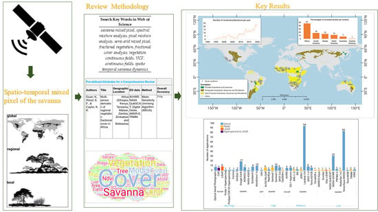
2. Review Methodology

For relevant literature to be identified, the Web of Science and Google Scholar were searched using the following singular or set of combined key words: “savanna mixed pixel”, ”spectral mixture analysis”, ”pixel mixture analysis”, ”semi-arid mixed pixel”, ”dryland mixed pixel”, ”mixed pixel”, ”sub-pixel”, ”pixel-unmixing”, pixel decomposing”, ”fractional cover”, ”vegetation fractional cover”, ”fractional vegetation”, ”fractional cover analysis”, ”vegetation continuous fields”, ”VCF”; “continuous fields”, ”spatio temporal savanna dynamics”, ”remote sensing”, ”multi-spectral”, ”multi-temporal”, ”earth observation”, using “OR” to combine the terms. A wide range of key words were selected as the problem of mixed pixel is addressed by different, inconsistent, and interchangeably used terminologies. The search range time is between 1990 to 2020. This resulted in an initial total number of 4079 journal articles. The 4079 journal articles were screened further to form part of the final review according to the following criteria:
  • The journal article must be focused on mixed pixel analysis.
  • The journal article study area is located in a savanna biome.
  • The journal article is fully or in parts using EO as input data to derive single or multiple fractional land cover.
  • A number of global VCF articles and very few articles with focus on semi-arid or dryland biomes, such as grasslands and savanna desert ecotones, were considered. Vegetation Continuous Fields methods are fundamental to the development of fractional and sub-pixel mapping, although not entirely focusing on the savanna most of the time.
After the screening process, 197 publications were retained for the final review process (Supplementary Materials Table S1). The retained papers were further analyzed and their pre-defined parameters and attributes extracted to form part of the in-depth analysis. The parameters extracted and analyzed are the year of publication, journal name, geographic location of the study area, spatial extent of the study area, type of EO data used (i.e., sensor mission name, sensor platform type, spatial resolution, temporal resolution), method of estimation, type of biophysical parameters estimated, characteristics of the input data, EO data used for validation data, and the overall accuracy of the EO data used for mixed pixel analysis.

3. Results

Figure 2 illustrates the list of journals included in the literature review. Majority of the papers were published across 10 high impact journals, with the journal of Remote Sensing of Environment having the highest number of published manuscripts. The “Others” category of journals is made up of journals containing only one publication.

3.1. Geographic and Spatial Scale

The geographic locations of the reviewed publications study areas are depicted in Figure 3. About 47% of the papers have a study area located in Africa, followed by South America with 18%. This is possibly because more than 50% of Africa is covered by savanna, concentrated in different parts of the continent and made up of varying savanna ecosystems.
The African savannas range from the Serengeti grassland savannas with scattered trees in East Africa (Kenya and Tanzania), to humid savannas in West Africa, dryland savannas of the Sahel region which are savanna desert ecotones, Miombo savanna woodlands, and semi-arid savannas in Southern Africa. The second highest number of studies focusing on Southern America can be justified by the fact that the continent is home to the Cerrado and Caatinga grasslands. The Cerrado, for example, is considered one of the global biodiversity hot-spots and one of the most diverse tropical savannas in the world [91]. These two biomes are recognized as biosphere reserves due to high level of species biodiversity, but, at the same time, they both have a high rate of fragmentation and are reported to be highly endangered due to high rates of deforestation and habitat fragmentation due to agriculture [10]. About 55% of the Cerrado’s original vegetation has been estimated by remote sensing to have been already converted by human actions [10]. The Caatinga biome, on the other hand, is reported to be one of the most threatened tropical ecosystems, with a greatest destruction rate [10]. Between 30.4% and 51.7% of the Caatinga is reported to be altered by human activities, making it as the third most heavily impacted biome in Brazil [92]. The Chaco and the Caatinga are considered to the most endangered biome in Brazil, at a risk of disappearing, which highlights an urgent priority for conservation due to great deforestation there [93]. About 8% of study sites were based in Australia. Only about 1% of the retained papers focus on Central America. The global category includes mainly the VCF literature, which are widely applied for estimation of global trees fractional cover by Hansen et al. [60,66,67,76,94,95,96]. Vegetation Continuous Fields are crucial in showing development and progress for fractional cover estimation but are mainly presented at a global scale and are derived from low spatial resolution remote sensing and are not necessarily focusing on savanna biomes alone [65,66].
The number of published mixed pixel studies in the savannas have increased in recent years. There is a peak in the number of studies in 2019, representing 11% of the total number of studies, and 10% of the studies were conducted in 2020 (Figure 3). The trend of increasing studies is less clear between 1994 and 2010; however, it is more pronounced between 2010 and 2020. Approximately 63% of the reviewed papers fall in the last 9 years of the 27 years length of the review period. This may be due to the increased availability and free accessibility of remote sensing data and the introduction of machine learning algorithms to successfully process big data reported in the last decade. A review on machine learning applications to land cover classification based on multispectral earth observation found more or less the same trend of number of publications doubling between 2015 to 2020 [97]. In addition, Wulder et al. [98] reported the emergence of a new era of land cover analysis, which is made possible by free access data and ready-to-analyze EO data along with the availability of high-performance computer processing capabilities to enable rapid data processing.
The vast majority of the studies (~63%) were conducted at a local scale (Figure 4). Approximately 24% of the reviewed publications were conducted at a regional scale.
Regional scale represents studies with a study area located in more than one neighboring country or where more than one country is included in the study area. Only about 6% of studies were conducted at a global scale, 5% at a national scale, and 2% at a continental scale (Figure 4). Data processing and storage power has increased, but it seems that working with EO data at continental and global scale remain a challenge [99]. Another reason could also be because savannas are so variable at large scales, and, hence, methods must be developed and calibrated at smaller scales. Savanna mixed-pixel analysis of vegetation components often requires multi-temporal images spanning over several seasons to capture phenological differences in order to increase accuracy [5]. These multi-temporal images are required to go through pre-processing, which increases the computational demand [99]. At a global scale, generating and collecting reliable and geographically representative validation data tend to be a challenge. Besides the MODIS VCF studies which offer global fractional tree cover products [59,100], we identified only one study which conducted mixed pixel analysis of savannas at a global scale. Hill and Guerschman [11] used MODIS to characterize vegetation fractional cover with a focus on grasslands and savannas at a global scale. In addition, Jia et al. [101] used a general regression neural networks algorithm on MODIS data to estimate land surface fractional vegetation cover on a global scale. There was no study found at a sub-national regional level to qualify as regional at a single country level. A few of the regional scale studies were conducted in African savanna mosaics along the Sahel drylands of West Africa with several countries, such as Mali and Niger, included in the study area [102,103,104]. For example, Souverijns et al. [105] estimated fractional land cover over a period of 30 years at a regional scale in Senegal, Burkina Faso, Nigeria, Niger, and Sudan. In other regions, Guan et al. [106] estimated vegetation fractional land cover over tropical savanna regional areas covering Ethiopia, Kenya, Tanzania, Malawi, Zambia, Zimbabwe, and Botswana.

3.2. Estimated Mixed-Pixel Parameters

The majority of the reviewed studies (62%) estimated multiple fractional covers when analyzing mixed pixels (Figure 5). Multiple cover estimation means that the authors did not just focus on estimating one type of cover but estimated multiple fractional covers, such as grass, trees, shrubs, and bare ground, or various combinations of these. Theseira et al. [107] estimated multiple fractional covers by applying a spectral mixture model to derive grassland, areas of low and high savanna trees, grassland, savanna shrub, and bare ground; Xian et al. [108] used non-parametric regression trees to characterize a shrubland environment into continuous fields of herbaceous, litter, shrub, and bare ground; and Bauman et al. mapped continuous fields of tree and shrub cover in the Gran Chaco savanna ecosystem in South America [109]. Trees were the most estimated single fractional cover. Approximately 20% of the reviewed studies estimated tree cover (Figure 5). Hansen et al. [60,61] estimated global tree VCF. It is possible that there can be overlap between tree cover and woody cover, since woody cover may include trees and shrubs. This is further confounded by tree cover and woody cover often being used as interchangeable terms, as well as the differences between studies in defining the difference between a tree and a shrub (e.g., criteria of height and multi-stemming). Roughly 13% of the reviewed papers estimated woody fractional vegetation cover, which typically includes both tree and shrub cover (Figure 5). Many studies estimated woody cover in African savannas [84,110]. For example, Higginbottom et al. [111] and Naidoo et al. [83] used a fusion of optical data with SAR to estimate fractional woody cover in African savanna. In other regions, Yang and Crew [48] used Landsat data to estimate woody cover in the Texas savannas in North America.

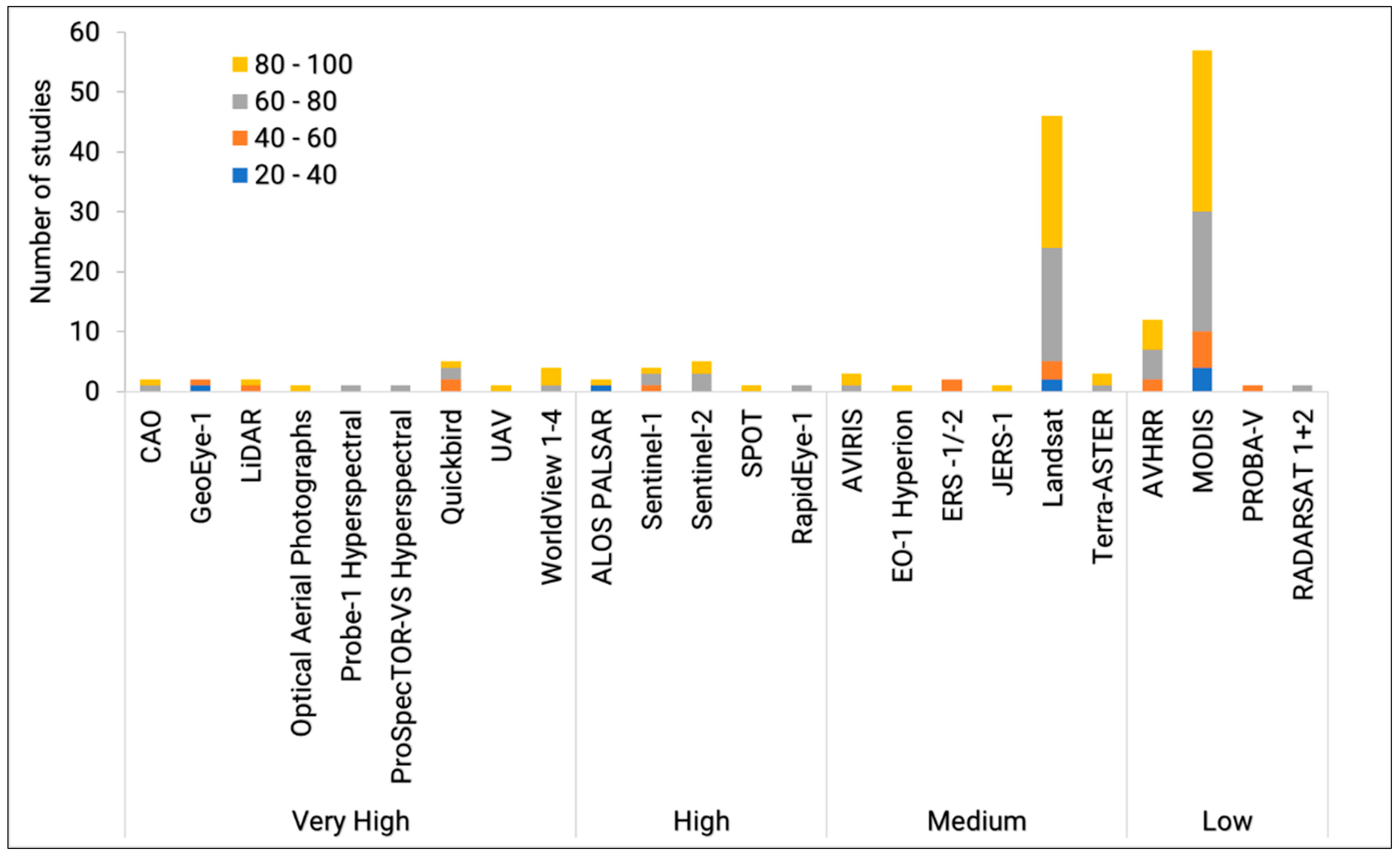
3.3. Type of Earth Observation Data Used

In many scenarios, there are multiple EO data types employed by a single paper. For example, Gessner et al. [112] employed a multi-resolution approach that included four different sources of remote sensing data (Quickbird-2, IKONOS-2, Landsat TM, and MODIS) to derive fractional cover at a regional scale in an African grassland, savanna, and shrubland biome.
Additionally, the overview shows the employed EO sensor systems classified according to optical, radar, LiDAR, or LiDAR and hyperspectral (Figure 6). Spatial resolution is classified from very high to low resolution.
A total of 39 EO data types were used in the reviewed studies. This reflects a wide range of EO applications for savanna mixed pixel analysis [47,105,113,114,115,116,117,118]. Of these, 26 (89%) were optical, 11 (7%) radar, 2 (3%) LiDAR, and 1 (1%) were a combination of optical hyperspectral and LiDAR. The most frequently used EO data were optical Landsat (n = 94), MODIS (n = 83), AVHRR (n = 26), and Google earth (n = 22). These EO systems have a short return period, long time series, and are freely available. For example, Landsat, MODIS, and AVHRR have been in operation for more than 20 years, providing freely available and continuous EO data. Landsat has been providing data for thematic Land Use and Land Cover (LULC) mapping for more than 30 years now. Google Earth is not necessarily a sensor fleet but is included in the list of EO data used because, as a very high spatial resolution data, it has been used in many of the reviewed papers as a reference data for validation and accuracy assessments. Both MODIS and AVHRR datasets are well suited for large study area scenarios, as well as for applications where a long time series is most crucial. The major advantage of AVHRR in the spatio-temporal dynamics of the savanna mixed pixel analysis is that it offers long time series spanning as far back as 1981. AVHRR, regardless of it being known for its broad channels and that AVHRR Vegetation Indices (VIs) products are reported to be less accurate when compared with MODIS VIs, long-term NDVI time series, AVHRR Global Inventory Modeling and Mapping Studies (GIMMS), have been found to be suitable for long-term vegetation studies in dry areas [119]. The long time series and high revisiting times of these low-resolution remote sensing data is effective to limit gaps in the time series as a result of cloud cover issues [120]. Creating consistent time series from very high and high spatial resolution data, however, is often not easy. This is because of their low revisiting and smaller area coverage. This probably explain why high and very high spatial resolution images are under-represented in the analysis of mixed pixel compared to low and medium spatial resolution with high revisiting time.
High spatial resolution (HR) and very high spatial resolution (VHR) sensors, such as IKONOS-2, Quickbird, GeoEye, and SPOT 5-6, have been applied less often. This is likely due to the low revisiting time and high data costs [121]. Historically, VHR and HR tend to have smaller swath coverage to be considered for large spatial scale studies compared to coarse and medium resolutions. Low temporal resolution tends to be less suitable for tracking seasonal dynamics in the vegetation [121]. The aspect of seasonal variation is often influential in the separability of vegetation components in the mixed pixel analysis of the savanna [11].
Synthetic Aperture Radar (SAR) played a very minor role in the type of EO sensor data used. This is despite the fact that SAR data tends to be a better option for multi-temporal mixed pixel analysis because it is not severely affected by most weather conditions and is unaffected by cloud cover. Furthermore, the limited application of SAR may also be due to computational challenges given the spatial and spectral distortions and geometric distortions as a result of the complex nature of processing SAR [122]. Within the reviewed publications, there were fewer scenarios of fusion between SAR and optical EO data. This is despite the fact that studies that combined SAR with the optical reported higher accuracies compared to when SAR or optical were used alone. For instance, Baumann et al. [109] developed a novel approach to map continuous fields of tree cover and shrub cover across the South American Gran Chaco, using Landsat-8 optical and SAR Sentinel-1. The study found that the best model for VCF estimation was the one which fused optical and SAR, performing far better than models using data from only one sensor. Borges et al. [123] used Sentinel-1 and Sentinel-2 to map savanna land cover, and Naidoo et al. [83] tested the utility of multi-seasonal and multi-sensor use of Landsat TM/ETM and ALOS PALSAR to map woody fractional cover over South Africa’s semi-arid savannas. All three studies reported higher and improved accuracies for models which integrated SAR with optical data [109,113].

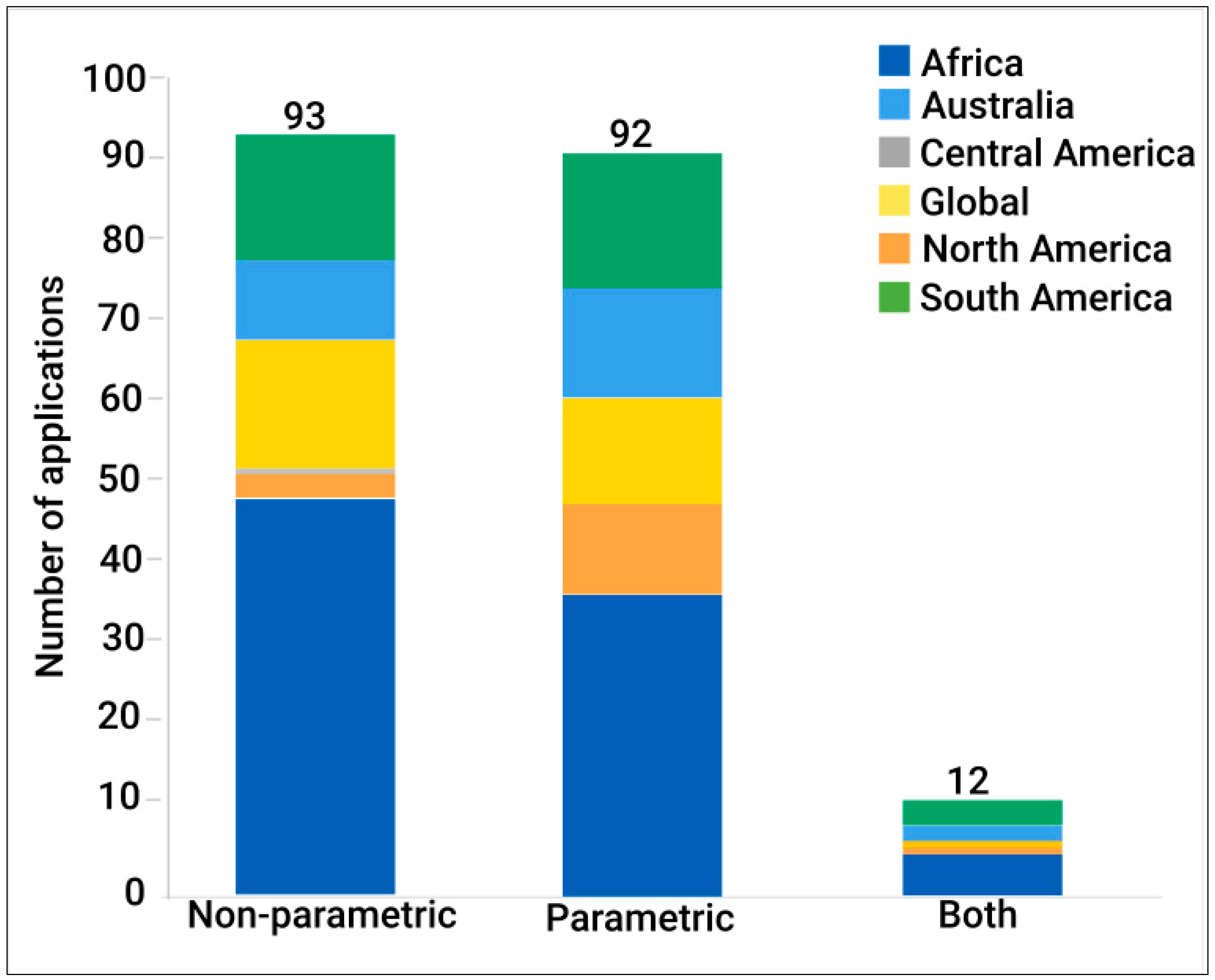
3.4. Methods Used for Estimation of Mixed Pixel Parameters

Categorization of Savanna Mixed Pixel Estimation Methods

Table 1 shows that various methods were used to estimate mixed pixel parameters using EO data. The identified methods were categorized into parametric and non-parametric approaches (Table 1). Maximum Likelihood (ML) classification is one of the parametric methods for categorical classification. Here, a gaussian normal distribution is assumed. For example, supervised classification is a parametric classification which assumes a multi-variate gaussian distribution of each class that is extracted from the training data by estimating the central tendency statistics, such as the mean and covariance matrix, which are used as the parameters for discrimination between land covers [124]. Parametric methods for categorical and discrete classifications include Step-wise Discriminant Analysis (DA) and Minimum Distance (MD). However, because these classifications only use decision boundaries, they tend to be prone to noisy classifications when applied in regions with high heterogeneity. Parametric classifications are reported to lack robust capabilities and tend to be unsatisfactory in characterizing land cover in large areas with complex environments, such as the savannas [124].
However, non-parametric classifiers side-step the parametric issues. Non-parametric methods use an iterative process. Examples of non-parametric classifiers include Nearest Neighbor (1-NN and k-NN), kernel methods [125], neural networks, and classification trees, Random Forest (RF) and Regression Trees (RT) [94]. Non-parametric methods, however, require more training data and are computationally intensive due to large sets of training data. Non-parametric methods are postulated to circumvent the issues of arbitrary boundaries. These issues are common in parametric methods. Non-parametric methods are reported to offer computational flexibility and are more robust to apply to processing of large areas data and well suited to areas where the distribution of the land cover is not well known [53]. Parametric methods, on the other hand, are unsatisfactory in large areas and, especially, in complex environments with no obvious land cover class gradient. Some publications employed both parametric and non-parametric methods (indicated as “Both” in Figure 7, Figure 8 and Figure 9 and Table 1).
Table 1. Examples of methods used for spatio-temporal mixed-pixel analysis. The methods are categorized as parametric, non-parametric, and both (a combination of parametric and non-parametric methods).
ReferenceMethod NameMethod TypeEstimated Biophysical Parameter
[75]Regression Tree(Non-parametric)Tree Cover
[126]Spectral Mixture Analysis (Pixel Unmixing)ParametricPercent vegetation cover per pixel (% woody vegetation, % herbaceous vegetation, % bare ground), leaf type (% needleleaf and % broadleaf) and leaf duration (% evergreen and % deciduous) and % bare
[39]Object-Based Image Analysis Nearest neighbor
Maximum Likelihood Random Forest
Regression Tree Support Vector Machines
Parametric and Non-parametric (Both)Multiple Cover: Trees, Shrubs, Bare Soils, Grass
[105]Random ForestNon-parametricMultiple Cover: Shrubland, Forest, Urban, Cropland, Seasonal water, Bare Soil, Permanent water
In Figure 7, the literature review shows the percentage of applications for each method categorization. The review shows that 93 (~47%) of the reviewed publications used non-parametric methods, while 92 (~47%) used parametric methods, and only 12 (~6%) used a combination of parametric and non-parametric methods.
From a geographic perspective (Figure 8), non-parametric methods have the highest percentage of application in Africa, with more than 50% of the studies having used non-parametric methods located in Africa. When it comes to Australia, studies conducted in Australia have a slightly higher preference of parametric methods of ca. 11% use compared to ~2.5% application of non-parametric methods there. Due to Africa having a range of savanna ecosystems with high cover variability due to variable fire regimes and land uses (e.g., livestock grazing and wildlife conservation), the high variability in cover may prompt researchers to opt for methods which are capable of dealing with high spatial heterogeneity in land cover [15].
When we observed the type of methods from VHR to low spatial resolution in Figure 9, we found non-parametric methods to be the most frequently applied to VHR and HR EO systems with 60% and 77%, respectively. Contrary to that, parametric method were the most frequently used methods for medium and low resolution EO data with 55% and 51% application there, respectively. Generally, we found that, for EO sensors falling in the categories of VHR and HR, approximately more than half 11 (57%) of them have more than 50% of non-parametric methods application. Apart from MODIS, sensors of medium and low resolution tend to have employed parametric methods more frequently.

3.5. Temporal Characteristics of the EO Input Data

Figure 10 represents the type of input EO data attributes for spatio-temporal mixed pixel analysis of savannas. The two most widely used EO input data attributes are band statistics (40%) and spectral indices (28%) (Figure 10a). For this review, band statistics consists of metrics from spectral bands and metrics from indices, such as maximum band value, mean of NDVI, mean of reflectance, maximum NDVI value, mean band value, standard deviation NDVI value, and amplitude band value. Vegetation indices are used as a proxy for vegetation cover in spatio-temporal mixed pixel studies. Many of the normalized indices used red reflectance and NIR and applied parametric linear regression methods, SMA, non-parametric time series decomposition trend methods, such as harmonic analysis or machine learning methods, for mixed pixel parameters estimation [127,128,129,130]. The third most used data input is seasonal metrics (14%). Seasonal metrics correspond to those input data whose spectral values correspond to phenological cycles and stages in the spectral or reflectance metrics or indices, for example, NDVI peak greenness, value rate of green up, total length of growing season, the timing of the onset of green up, and the onset of the maximum NDVI.
The majority of the studies used inter-annual (68%) temporal data, which means the time series enabled the modeling of inter-annual differences of multiple years (Figure 10b). The majority of the temporal EO data used in the mixed pixel analysis are multi-temporal time series (77%) (Figure 10c). A larger part of the studies applied shorter time series (~61.4%) EO data with a length of 1–5 years in (Figure 10d).
The length of investigation for each reviewed paper was examined (Figure 11). The starting year and the ending year analysis are considered to derive the paper’s study period (x-axis) and the publication year (y-axis). The results show that many studies have used multiple years to understand the spatio-temporal dynamics of the mixed pixel. More than 60% of the reviewed papers used data spanning over multiple years to look into the spatio-temporal dynamics of the mixed pixel. However, the majority of those studies have a length of investigation between 1 to 5 years, which indicates a leaning towards use of shorter time series. The longest study period is 59 years, which analyzed long archives of optical aerial photographs combined with satellite data to assess woody vegetation spatio-temporal dynamics in South Africa [131]. Blentlinger and Herrero [132] also characterized woody cover in a protected area for over 44 years in a neotropical savanna ecosystem in Belize, Central America.

3.6. Accuracy and Validation of the Reviewed Publications

In Figure 12, the accuracy of the reviewed studies which reported a clear overall accuracy is summarized. Overall accuracy considered for the analysis means the study reported a standard accuracy metric of either confusion matrix overall accuracy, kappa, or a R2 from a regression model. About 85% of the reviewed studies reported a clear overall accuracy. For the papers which reported an overall accuracy, the majority (46%) have an accuracy class between 80–100% (Figure 12a). For the studies which reported an overall accuracy, EO datasets used as reference data for accuracy assessment are shown (Figure 12b).
In order to find out which EO datasets achieved a better accuracy, a comparison is made between the four accuracy categories (Figure 13) across the spatial resolutions (very high, high, medium, and low) of those EO datasets utilized by the studies. The EO dataset types which have the highest percentage of studies achieving a >60% accuracies are those which have used medium spatial resolution (88%), followed by 84% of studies which have used the HR spatial resolution EO data. Studies which used VHR EO data have the lowest (74%) number of studies, which achieved accuracies of >60%, followed by those studies which have used low spatial resolution EO data (82%). The majority of studies have used low spatial resolution compared to others, with HR EO datasets being the least used across those studies which reported an overall accuracy. Although less frequently used, HR studies achieved better accuracies compared to VHR and low resolution. Medium resolution studies which have the highest percentages of studies (88%), with high accuracies (>60%), is the second most used type of EO datasets across the 159 studies that have reported an overall accuracy and the most used EO data type among all the 197 reviewed studies.
For the three method categories used for mixed pixel analysis in Figure 14, 90% of the studies which have used more than one method type achieved >60% accuracy, followed by 87% of studies which used only parametric methods, and 79% of studies which used only non-parametric methods. Although all methods have a high percentage of papers achieving >60% accuracies, those papers which applied more than one method seem to have performed the best by a small margin. This is regardless of the fact that fewer papers have used a combination of methods.

4. Discussion

4.1. Geographic Patterns of Spatio-Temporal Mixed Pixel Analysis in the Savannas

Because of their large spatial extend and since they are a prime target for conversion from their natural states to agriculture, the provision of rangelands for livestock and subsistence for native populations, majority of the studies have been conducted in the African and South American savannas (Figure 3) [3,5,14,28,30,32,36,38,39,46,47,52,86,95,106,112,114,116,117,118,129,130,133,134,135,136,137,138,139,140,141,142,143,144,145,146,147,148,149,150,151,152,153,154,155,156,157,158,159,160,161,162,163,164,165,166]. The African and Southern American savannas have a significant role in vegetation trends as a result of interactions by climate change and increasing carbon dioxide [15]. The Cerrado, along with the Caatinga, is one of the important savanna or dryland biomes of South America which have very rich flora and high endemism but only have each roughly 2.2% and 1% of their area protected for conservation, respectively, by the year 2015 [91]. The Cerrado, due to mechanized agriculture, conversion for human occupation, invasive grasses, and uncontrolled fires, is going through an intensification of anthropogenic processes, which is a major threat to biodiversity [10]. The Caatinga biome, at the same time, is also undergoing human density, replacement of gallery and dry forests due to desertification, charcoal production, timber, and cattle ranching [10].
The majority of mixed pixel analysis of the savanna have been conducted at the local and regional level with very few studies at a global and continental scale (Figure 4). Mixed pixel analysis at larger spatial scales, such as continental and global scale, tend to be a challenge which lead to more studies focusing at local spatial scales [43]. This is due to the fact that land cover trends tend to differ in some ecoregions due to climate and land use [11]. These difference in land cover trends occur in specific ecoregions and will require more detailed analysis at fine spatial and temporal scales for better understanding. Studies on mixed pixels found that regions with high heterogeneity are a challenge for analysis. Accounting for inherent heterogeneity in savannas, areas of transitional zones between major ecosystems, areas with major anthropogenic activities, boreal forests and tundra, and mountain range areas is reported to be a major challenge. When classifying biomes heterogeneity from high to low, the savanna biome is ranked the highest in terms of heterogeneity [43]. Since 64% of the global vegetated areas are reported to be a mixture of vegetation cover types, this is an indication that much of the global land surface is faced with mixed pixel and high heterogeneity. The majority of the mixed pixels are also composed of cover types with different vegetation heights especially in transitional ecological zones [43]. Land surfaces in savanna biomes at a global scale are not uniform but highly diverse and heterogenous. This means that robust methods to account for site differences and the mixed nature of covers are required when analyzing savanna at a global and continental scale to account for the variations in cover. It is possibly because of the obstacles in analysis of the savanna at continental and global scale which led to more studies to focus analysis at savanna local spatial scale. At local scales, the complexity may not be as comparable to large area analysis, as there is less probability of different ecosystems occurring at a local scale.

4.2. The Use of EO Technology for Spatio-Temporal Mixed Pixel Analysis in Savannas

Optical EO data were utilized more often with medium spatial resolution (30 m) Landsat being the single majority applied sensor for spatio-temporal mixed-pixel analysis of the savanna (Figure 6) [83,113,114,166]. Landsat as the most commonly used EO sensor offers at least three decades of imagery with medium spatial resolution. Landsat provides consistent measurements of inter-annual variability of vegetation over the entire earth’s surface and the same will be assumed for the savanna ecosystems [120,167]. However, Landsat does not capture adequate intra-annual or phenological variability because of the 16-day interval for image acquisition [52,139].
The wide use of optical data comes with an under-representation of other EO technologies, such as Synthetic Aperture Radar (SAR) and LiDAR, in spatio-temporal mixed pixel analysis of the savanna. For improved classification, long-time series are required and integration of SAR and LiDAR with optical time series to improve classifications in the savanna is highly recommended [15]. SAR offers an added advantage to optical time series because it is largely weather independent. SAR has been used alone [84,85,166,168,169] and sometimes together with optical imagery [83,113,114,118]. Improved accuracies are reported when models use SAR or when SAR and optical are combined in the spatio-temporal mixed pixel analysis of the savanna [83,109]. Radar remote sensing does not depend on sun illumination or cloud condition and, therefore, is a good potential to offer continuous time series of EO data for long term monitoring of the savannas.
Most of the studies used short time series EO data for savanna spatio-temporal mixed pixel analysis (Figure 10d and Figure 11) [28]. Reliable spatio-temporal trends of the savannas require long time series [29,119,130,170]. EO sensors with many years of data archives are already available. This review has highlighted that the most preferred EO systems are those with a long history of existence. However, it seems the potential of long time series are not fully exploited so far in understanding the mixed pixel dynamics of the savanna. The satellite EO systems with long time series tend to be those with medium to low spatial resolution. The solution may be to fuse and harmonize long time series of low and medium spatial resolution (MODIS, AVHRR, and Landsat) with very high spatial resolution EO satellite data, such as the newly launched Sentinel-1 and Sentinel-2, for longer time series exploits; to fuse radar and optical remote sensing data and explore the recently launched HR EO datasets, such as the Sentinel-1 and Sentinel-2, for improved estimation of the savanna mixed pixel. The heterogenous nature of the savanna mixed pixel requires a consideration of high spatial, spectral, temporal, and radiometric resolution for accurate separation between savanna components.

4.3. Future Outlook

The rapid increase in the availability of data for land cover characterization offers great potential for contributing to new land surface cover information. However, this potential requires improved analysis methods beyond the use of vegetation indices and transformation of images. Big data is now more prevalent and open source data mining tools are readily available [171]. The recent launch of sensors with improved spatial and temporal resolutions, such as the Sentinel-1 and Sentinel-2 [118,143]; application of big data processing [143]; and the combination of SAR, LiDAR, and optical data [118] signals the future direction of remote sensing of savanna environments from space. Multi-sensor, multi-scale imaging is recommended, especially for three-dimensional characterization of the savanna [11].
Cloud computing platforms, such as the Google Earth Engine (GEE), are reported to be a milestone in creating robust reference data to train ML algorithms for analysis in mixed and highly seasonal ecosystems, especially where reference maps for time series classifications are inadequate or unavailable [98,143]. GEE is a powerful tool which brings together multitudes of EO datasets for analysis. The GEE platform offers remarkable computational power with ready-to-analyze data available. Cloud platforms, such as GEE, have the potential to process data that requires high computational power since the process do no take up hard disk space on the computer, thus providing a potential opportunity to perform analysis at continental or global scale and counter-act the issue of data complexities and the lack of studies at large scales (i.e., global and continental) in savanna ecosystems. The GEE platform is especially well suited to large scale analysis in developing countries where access to advanced computational and data processing facilities is a challenge.

5. Conclusions

Estimating mixed pixel parameters in the savanna is essential for long-term understanding of the spatio-temporal dynamics and trends. Mixed pixel vegetation cover is an important biodiversity parameter in savannas where the estimation of the above ground biomass in savanna varies according to fraction of the trees, shrubs, and grasses. The review shows that the spatial focus of the spatio-temporal mixed pixel analysis is on the African and South America savannas due to the size and the importance of biodiversity conservation in the two regions. The majority of the studies are conducted at a local and regional scale which highlights a gap for studies at national, continental, and global scale. The gap in studies at the larger scales (continental and global), in addition, means that robust methods which are capable of large data analysis and handling the complex and highly heterogenous nature of the savanna are required. The preference to use medium (Landsat) and low (AVHRR and MODIS) spatial resolution optical EO datasets highlights the gap in use of high spatial resolution and radar remote sensing to estimate the mixed pixel of the savanna. In addition, the use of short time series of up to 5 years maximum emphasizes that long time series data which are essential for understanding spatio-temporal dynamics of the savannas are required in the estimation of the mixed pixel of savannas.
Although there was no difference in the use of parametric versus non-parametric methods, the preference to apply non-parametric methods when analyzing high spatial resolution EO indicates that more robust non-parametric methods are required to deal with the large scale EO datasets and the required high spatial resolution data to understand the spatio-temporal dynamics of the savanna mixed pixel. The increase in the use of non-parametric methods, for example, Random Forest machine learning methods, mainly used to estimate fractional woody cover in the African savannas, is a good example. Non-parametric methods, such as regression tree methods, are used mainly by the VCF studies which estimated global VCF tree cover probably due to their robustness and ability to handle large volume of data. The most used input data band statistics which are composed of mainly multi-temporal composites which capture phenology to separate savanna vegetation components shows that a multitude of temporal data are required for spatio-temporal dynamics of the savanna. It also indicates that understanding the spatio-temporal analysis of the savanna requires a large volume of data, along with big data infrastructures to handle them. The majority of the time series used are of inter-annual nature, however, consisting of rather short analysis periods. Therefore, the review highlights a research gap for savanna spatio-temporal mixed pixel analysis using high-resolution long time series. This gap can be addressed by increasing the incorporation of active EO, such as SAR. Optical EO data with long time series, such as Landsat, can be harmonized with the recently launched high resolution Sentinel-1 and Sentinel-2 sensors. In addition, exploring the fusion of high-resolution SAR and optical to address the gaps in time series data due to cloud cover is also a possibility. Satellite data are increasingly becoming available. This creates opportunities for big data and open-source data mining tools to be created, especially to provide fitting methods to monitor complex ecosystems, such as the savanna. The review set out to find out the type of EO datasets and methods used for mixed pixel analysis of the savanna and found a gap for high-resolution EO datasets. This indicate that although satellite data is increasingly available, the processing capabilities of high spatial resolution remote sensing data to monitor long term changes for savannas may be a challenge, especially at global and continental scales. When it comes to EO datasets and what type of methods they recruit for mixed pixel analysis and how accurate they tend to be, it seems that combinations of parametric and non-parametric methods are recommended, along with medium and high spatial resolution long time series EO datasets, for a more accurate spatio-temporal mixed pixel analysis of the savanna.

Supplementary Materials

The following are available online at https://www.mdpi.com/article/10.3390/rs13193870/s1, Table S1: List of all reviewed research articles.

Author Contributions

Conceptualization, H.S.N., M.U. and C.S.; Formal analysis & investigation: H.S.N. with assistance of M.U.; Writing-original draft preparation, H.S.N.; Review and editing, H.S.N., M.U., C.S., J.B., A.R., B.M. and I.P.J.S.; Supervision, M.U. and C.S. All authors have read and agreed to the published version of the manuscript.

Funding

The study is made possible by funding from the Deutscher Akademischer Austauschdienst: DAAD Ref No. SPACES II.2 CaBuDe 57531823. The work benefited from funding by the Federal Ministry of Education and Research (BMBF) under the project ‘SPACES2 Joint Project: South Africa Land Degradation Monitor (SALDi)’ (BMBF funding code: 01LL1701A) within the framework of the Strategy “Research for Sustainability” (FONA) www.fona.de/en.

Data Availability Statement

The data is available in the article and in the supplementary material. Supplementary data provided contains the data which is presented in the study.

Acknowledgments

Our utmost acknowledgements go to Sophie Reinnerman from the German Aerospace Center (DLR) for her provision of python code which enabled the analysis to generate Figure 11.

Conflicts of Interest

There is no declared conflict of interest from the authors.

Abbreviations

AVHRRAdvanced Very High-Resolution Radiometer
EOEarth Observation
GEEGoogle Earth Engine
GIMMSGlobal Inventory Modeling and Mapping Studies
HRHigh Resolution
INPENational Institute for Space Research
1/k-NNNearest Neighbor
LULCLand Use Land Cover
MDMinimum Distance
MAPMean Annual Precipitation
MATMean Annual Temperature
MLMachine Learning
MODISModerate Resolution Imaging Spectroradiometer
NDVINormalized Difference Vegetation Index
RFRandom Forest
RTRegression Tree
SAEONSouth African Environmental Observation Network
SARSynthetic Aperture Radar
SDAStep-wise Discriminant Analysis
SMASpectral Mixture Analysis
VCFVegetation Continuous Fields
VHRVery High Resolution
VIVegetation Indices
VIIRSVisible Infrared Imaging Radiometer Suite

References

  1. Scholes, R.J.; Archer, S.R. Tree-Grass Interactions in Savannas. Annu. Rev. Ecol. Syst. 1997, 28, 517–544. [Google Scholar] [CrossRef]
  2. Sankaran, M.; Hanan, N.P.; Scholes, R.J.; Ratnam, J.; Augustine, D.J.; Cade, B.S.; Gignoux, J.; Higgins, S.I.; le Roux, X.; Ludwig, F.; et al. Determinants of Woody Cover in African Savannas. Nature 2005, 438, 846–849. [Google Scholar] [CrossRef]
  3. Herrero, H.; Southworth, J.; Muir, C.; Khatami, R.; Bunting, E.; Child, B. An Evaluation of Vegetation Health in and around Southern African National Parks during the 21st Century (2000–2016). Appl. Sci. 2020, 10, 2366. [Google Scholar] [CrossRef] [Green Version]
  4. Herrero, H.V.; Southworth, J.; Bunting, E.; Kohlhaas, R.R.; Child, B. Integrating Surface-Based Temperature and Vegetation Abundance Estimates into Land Cover Classifications for Conservation Efforts in Savanna Landscapes. Sensors 2019, 19, 3456. [Google Scholar] [CrossRef] [PubMed] [Green Version]
  5. Nagelkirk, R.L.; Dahlin, K.M. Woody Cover Fractions in African Savannas from Landsat and High-Resolution Imagery. Remote Sens. 2020, 12, 813. [Google Scholar] [CrossRef] [Green Version]
  6. Angassa, A.; Oba, G. Effects of Grazing Pressure, Age of Enclosures and Seasonality on Bush Cover Dynamics and Vegetation Composition in Southern Ethiopia. J. Arid Environ. 2010, 74, 111–120. [Google Scholar] [CrossRef]
  7. Sankaran, M. Droughts and the Ecological Future of Tropical Savanna Vegetation. J. Ecol. 2019, 107, 1531–1549. [Google Scholar] [CrossRef] [Green Version]
  8. Ma, X.; Huete, A.; Yu, Q.; Coupe, N.R.; Davies, K.; Broich, M.; Ratana, P.; Beringer, J.; Hutley, L.B.; Cleverly, J.; et al. Spatial Patterns and Temporal Dynamics in Savanna Vegetation Phenology across the North Australian Tropical Transect. Remote Sens. Environ. 2013, 139, 97–115. [Google Scholar] [CrossRef]
  9. Feldt, T.; Karg, H.; Kadaouré, I.; Bessert, L.; Schlecht, E. Growing Struggle over Rising Demand: How Land Use Change and Complex Farmer-Grazier Conflicts Impact Grazing Management in the Western Highlands of Cameroon. Land Use Policy 2020, 95, 104579. [Google Scholar] [CrossRef]
  10. Werneck, F.P. The Diversification of Eastern South American Open Vegetation Biomes: Historical Biogeography and Perspectives. Quat. Sci. Rev. 2011, 30, 1630–1648. [Google Scholar] [CrossRef]
  11. Hill, M.J.; Guerschman, J.P. The MODIS Global Vegetation Fractional Cover Product 2001–2018: Characteristics of Vegetation Fractional Cover in Grasslands and Savanna Woodlands. Remote Sens. 2020, 12, 406. [Google Scholar] [CrossRef] [Green Version]
  12. Zhou, Q.; Liu, S.; Hill, M.J. A Novel Method for Separating Woody and Herbaceous and Time Series. Photogramm. Eng. Remote Sens. 2019, 85, 509–520. [Google Scholar] [CrossRef]
  13. Zhou, Q.; Hill, M.; Sun, Q.; Schaaf, C. Retrieving Understorey Dynamics in the Australian Tropical Savannah from Time Series Decomposition and Linear Unmixing of MODIS Data. Int. J. Remote Sens. 2016, 37, 1445–1475. [Google Scholar] [CrossRef]
  14. Tsalyuk, M.; Kelly, M.; Getz, W.M. Improving the Prediction of African Savanna Vegetation Variables Using Time Series of MODIS Products. ISPRS J. Photogramm. Remote Sens. 2017, 131, 77–91. [Google Scholar] [CrossRef] [Green Version]
  15. Hill, M.J. Remote Sensing of Savannas and Woodlands: Editorial. Remote Sens. 2021, 13, 1490. [Google Scholar] [CrossRef]
  16. Archibald, S.; Scholes, R.J.; Roy, D.P.; Roberts, G.; Boschetti, L. Southern African Fire Regimes as Revealed by Remote Sensing. Int. J. Wildland Fire 2010, 19, 861–878. [Google Scholar] [CrossRef] [Green Version]
  17. Oliveras, I.; Malhi, Y. Many Shades of Green: The Dynamic Tropical Forest–Savannah Transition Zones. Philos. Trans. R. Soc. B Biol. Sci. 2016, 371, 20150308. [Google Scholar] [CrossRef] [Green Version]
  18. Moncrieff, G.R.; Scheiter, S.; Bond, W.J.; Higgins, S.I. Increasing Atmospheric CO2 Overrides the Historical Legacy of Multiple Stable Biome States in Africa. New Phytol. 2014, 201, 908–915. [Google Scholar] [CrossRef]
  19. Buitenwerf, R.; Bond, W.J.; Stevens, N.; Trollope, W.S.W. Increased Tree Densities in South African Savannas: >50 Years of Data Suggests CO2 as a Driver. Glob. Chang. Biol. 2012, 18, 675–684. [Google Scholar] [CrossRef]
  20. Bond, W.J.; Midgley, G.F. Carbon Dioxide and the Uneasy Interactions of Trees and Savannah Grasses. Philos. Trans. Soc. B Biol. Sci. 2012, 367, 601–612. [Google Scholar] [CrossRef] [Green Version]
  21. Archibald, S.; Scholes, R.J. Leaf Green-up in a Semi-Arid African Savanna-Separating Tree and Grass Responses to Environmental Cues. J. Veg. Sci. 2007, 18, 583–594. [Google Scholar] [CrossRef]
  22. Archibald, S.; Bond, W.J.; Hoffmann, W.; Lehmann, C.; Staver, C.; Stevens, N. Distribution and determinants of savannas. In Savanna Woody Plants and Large Herbivores; John Wiley & Sons, Ltd.: London, UK, 2019; pp. 1–24. ISBN 9781119081111. [Google Scholar]
  23. Higgins, S.I.; Bond, W.J.; Trollope, W.S.W. Fire, Resprouting and Variability: A Recipe for Grass–Tree Coexistence in Savanna. J. Ecol. 2000, 88, 213–229. [Google Scholar] [CrossRef]
  24. Staver, A.C.; Archibald, S.; Levin, S. Tree Cover in Sub-Saharan Africa: Rainfall and Fire Constrain Forest and Savanna as Alternative Stable States. Ecology 2011, 92, 1063–1072. [Google Scholar] [CrossRef]
  25. Stevens, N.; Lehmann, C.E.R.; Murphy, B.P.; Durigan, G. Savanna Woody Encroachment Is Widespread across Three Continents. Glob. Chang. Biol. 2017, 23, 235–244. [Google Scholar] [CrossRef] [Green Version]
  26. Osborne, C.P.; Charles-Dominique, T.; Stevens, N.; Bond, W.J.; Midgley, G.; Lehmann, C.E.R. Human Impacts in African Savannas Are Mediated by Plant Functional Traits. New Phytol. 2018, 220, 10–24. [Google Scholar] [CrossRef]
  27. Laris, P.S. Spatiotemporal Problems with Detecting and Mapping Mosaic Fire Regimes with Coarse-Resolution Satellite Data in Savanna Environments. Remote Sens. Environ. 2005, 99, 412–424. [Google Scholar] [CrossRef]
  28. Gaughan, A.E.; Holdo, R.M.; Anderson, T.M. Using Short-Term MODIS Time-Series to Quantify Tree Cover in a Highly Heterogeneous African Savanna. Int. J. Remote Sens. 2013, 34, 6865–6882. [Google Scholar] [CrossRef]
  29. Daldegan, G.A.; Roberts, D.A.; de Figueiredo Ribeiro, F. Spectral Mixture Analysis in Google Earth Engine to Model and Delineate Fire Scars over a Large Extent and a Long Time-Series in a Rainforest-Savanna Transition Zone. Remote Sens. Environ. 2019, 232, 111340. [Google Scholar] [CrossRef]
  30. Munyati, C.; Sinthumule, N.I. Assessing Change in Woody Vegetation Cover in the Kruger National Park, South Africa, Using Spectral Mixture Analysis of a Landsat TM Image Time Series. Int. J. Environ. Stud. 2013, 70, 94–110. [Google Scholar] [CrossRef]
  31. Salih, A.A.M.; Ganawa, E.-T.; Elmahl, A.A. Spectral Mixture Analysis (SMA) and Change Vector Analysis (CVA) Methods for Monitoring and Mapping Land Degradation/Desertification in Arid and Semiarid Areas (Sudan), Using Landsat Imagery. Egypt. J. Remote Sens. Space Sci. 2017, 20, S21–S29. [Google Scholar] [CrossRef]
  32. Mayes, M.T.; Mustard, J.F.; Melillo, J.M. Forest Cover Change in Miombo Woodlands: Modeling Land Cover of African Dry Tropical Forests with Linear Spectral Mixture Analysis. Remote Sens. Environ. 2015, 165, 203–215. [Google Scholar] [CrossRef]
  33. Gill, T.K.; Phinn, S.R. Improvements to ASTER-Derived Fractional Estimates of Bare Ground in a Savanna Rangeland. IEEE Trans. Geosci. Remote Sens. 2009, 47, 662–670. [Google Scholar] [CrossRef]
  34. Arroyo, L.A.; Johansen, K.; Armston, J.; Phinn, S. Integration of LiDAR and QuickBird Imagery for Mapping Riparian Biophysical Parameters and Land Cover Types in Australian Tropical Savannas. For. Ecol. Manag. 2010, 259, 598–606. [Google Scholar] [CrossRef]
  35. Johansen, K.; Arroyo, L.A.; Armston, J.; Phinn, S.; Witte, C. Mapping Riparian Condition Indicators in a Sub-Tropical Savanna Environment from Discrete Return LiDAR Data Using Object-Based Image Analysis. Ecol. Indic. 2010, 10, 796–807. [Google Scholar] [CrossRef]
  36. Okhimamhe, A.A. ERS SAR Interferometry for Land Cover Mapping in a Savanna Area in Africa. Int. J. Remote Sens. 2003, 24, 3583–3594. [Google Scholar] [CrossRef]
  37. Rian, S.; Xue, Y.; MacDonald, G.M.; Touré, M.B.; Yu, Y.; de Sales, F.; Levine, P.A.; Doumbia, S.; Taylor, C.E. Analysis of Climate and Vegetation Characteristics along the Savanna-Desert Ecotone in Mali Using MODIS Data. GISci. Remote Sens. 2009, 46, 424–450. [Google Scholar] [CrossRef] [Green Version]
  38. Marston, C.G.; Aplin, P.; Wilkinson, D.M.; Field, R.; O’Regan, H.J. Scrubbing Up: Multi-Scale Investigation of Woody Encroachment in a Southern African Savannah. Remote Sens. 2017, 9, 419. [Google Scholar] [CrossRef] [Green Version]
  39. Kaszta, Ż.; van de Kerchove, R.; Ramoelo, A.; Cho, M.A.; Madonsela, S.; Mathieu, R.; Wolff, E. Seasonal Separation of African Savanna Components Using Worldview-2 Imagery: A Comparison of Pixel- and Object-Based Approaches and Selected Classification Algorithms. Remote Sens. 2016, 8, 763. [Google Scholar] [CrossRef] [Green Version]
  40. Foody, G.M. Relating the Land-Cover Composition of Mixed Pixels to Artificial Neural Classification Output. Photogramm. Eng. Remote Sens. 1996, 62, 491–499. [Google Scholar]
  41. Whiteside, T.G.; Boggs, G.S.; Maier, S.W. Comparing Object-Based and Pixel-Based Classifications for Mapping Savannas. Int. J. Appl. Earth Obs. Geoinf. 2011, 13, 884–893. [Google Scholar] [CrossRef]
  42. Foody, G.M.; Mathur, A. The Use of Small Training Sets Containing Mixed Pixels for Accurate Hard Image Classification: Training on Mixed Spectral Responses for Classification by a SVM. Remote Sens. Environ. 2006, 103, 179–189. [Google Scholar] [CrossRef]
  43. Yu, W.; Li, J.; Liu, Q.; Zeng, Y.; Zhao, J.; Xu, B.; Yin, G. Global Land Cover Heterogeneity Characteristics at Moderate Resolution for Mixed Pixel Modeling and Inversion. Remote Sens. 2018, 10, 856. [Google Scholar] [CrossRef] [Green Version]
  44. Asner, G.P.; Wessman, C.A.; Privette, J.L. Unmixing the Directional Reflectances of AVHRR Sub-Pixel Landcovers. IEEE Trans. Geosci. Remote Sens. 1997, 35, 868–878. [Google Scholar] [CrossRef]
  45. Liu, Y.; Hill, M.J.; Zhang, X.; Wang, Z.; Richardson, A.D.; Hufkens, K.; Filippa, G.; Baldocchi, D.D.; Ma, S.; Verfaillie, J.; et al. Using Data from Landsat, MODIS, VIIRS and PhenoCams to Monitor the Phenology of California Oak/Grass Savanna and Open Grassland across Spatial Scales. Agric. For. Meteorol. 2017, 237–238, 311–325. [Google Scholar] [CrossRef]
  46. Hüttich, C.; Herold, M.; Strohbach, B.J.; Dech, S. Integrating In-Situ, Landsat, and MODIS Data for Mapping in Southern African Savannas: Experiences of LCCS-Based Land-Cover Mapping in the Kalahari in Namibia. Environ. Monit. Assess. 2011, 176, 531–547. [Google Scholar] [CrossRef]
  47. Schwieder, M.; Leitão, P.J.; da Cunha Bustamante, M.M.; Ferreira, L.G.; Rabe, A.; Hostert, P. Mapping Brazilian Savanna Vegetation Gradients with Landsat Time Series. Int. J. Appl. Earth Obs. Geoinf. 2016, 52, 361–370. [Google Scholar] [CrossRef]
  48. Yang, X.; Crews, K.A. Fractional Woody Cover Mapping of Texas Savanna at Landsat Scale. Land 2019, 8, 9. [Google Scholar] [CrossRef] [Green Version]
  49. Chu, D. Fractional Vegetation Cover. In Remote Sensing of Land Use and Land Cover in Mountain Region, 2nd ed.; Liang, S., Wang, J., Eds.; Academic Press: Cambridge, MA, USA, 2020; pp. 477–510. ISBN 978-0-12-815826-5. [Google Scholar]
  50. Liu, F.-J.; Huang, C.; Pang, Y.; Li, M.; Song, D.-X.; Song, X.-P.; Channan, S.; Sexton, J.O.; Jiang, D.; Zhang, P.; et al. Assessment of the Three Factors Affecting Myanmar’s Forest Cover Change Using Landsat and MODIS Vegetation Continuous Fields Data. Int. J. Digit. Earth 2016, 9, 562–585. [Google Scholar] [CrossRef]
  51. Gessner, U.; Machwitz, M.; Conrad, C.; Dech, S. Estimating the Fractional Cover of Growth Forms and Bare Surface in Savannas. A Multi-Resolution Approach Based on Regression Tree Ensembles. Remote Sens. Environ. 2013, 129, 90–102. [Google Scholar] [CrossRef] [Green Version]
  52. Ferreira, M.E.; Ferreira, L.G.; Sano, E.E.; Shimabukuro, Y.E. Spectral Linear Mixture Modelling Approaches for Land Cover Mapping of Tropical Savanna Areas in Brazil. Int. J. Remote Sens. 2007, 28, 413–429. [Google Scholar] [CrossRef]
  53. DeFries, R.S.; Townshend, J.R.G.; Hansen, M.C. Continuous Fields of Vegetation Characteristics at the Global Scale at 1-Km Resolution. J. Geophys. Res. Atmos. 1999, 104, 16911–16923. [Google Scholar] [CrossRef]
  54. Jeganathan, C.; Dadhwal, V.K.; Gupta, K.; Raju, P.L.N. Comparison of MODIS Vegetation Continuous Field—Based Forest Density Maps with IRS-LISS III Derived Maps. J. Indian Soc. Remote Sens. 2009, 37, 539–549. [Google Scholar] [CrossRef]
  55. Sarif, M.O.; Jeganathan, C.; Mondal, S. MODIS-VCF Based Forest Change Analysis in the State of Jharkhand. Proc. Natl. Acad. Sci. India Sec. A Phys. Sci. 2017, 87, 751–767. [Google Scholar] [CrossRef]
  56. Cartus, O.; Santoro, M.; Schmullius, C.; Li, Z. Large Area Forest Stem Volume Mapping in the Boreal Zone Using Synergy of ERS-1/2 Tandem Coherence and MODIS Vegetation Continuous Fields. Remote Sens. Environ. 2011, 115, 931–943. [Google Scholar] [CrossRef]
  57. Gao, Y.; Ghilardi, A.; Mas, J.-F.; Quevedo, A.; Paneque-Gálvez, J.; Skutsch, M. Assessing Forest Cover Change in Mexico from Annual MODIS VCF Data (2000–2010). Int. J. Remote Sens. 2018, 39, 7901–7918. [Google Scholar] [CrossRef]
  58. Hansen, M.C.; DeFries, R.S.; Townshend, J.R.G.; Carroll, M.; Dimiceli, C.; Sohlberg, R.A. Global Percent Tree Cover at a Spatial Resolution of 500 Meters: First Results of the MODIS Vegetation Continuous Fields Algorithm. Earth Interact. 2009, 7, 1–15. [Google Scholar] [CrossRef] [Green Version]
  59. Sexton, J.O.; Song, X.-P.; Feng, M.; Noojipady, P.; Anand, A.; Huang, C.; Kim, D.-H.; Collins, K.M.; Channan, S.; DiMiceli, C.; et al. Global, 30-m Resolution Continuous Fields of Tree Cover: Landsat-Based Rescaling of MODIS Vegetation Continuous Fields with Lidar-Based Estimates of Error. Int. J. Digit. Earth 2013, 6, 427–448. [Google Scholar] [CrossRef] [Green Version]
  60. Hansen, M.C.; Townshend, J.R.G.; DeFries, R.S.; Carroll, M. Estimation of Tree Cover Using MODIS Data at Global, Continental and Regional/Local Scales. Int. J. Remote Sens. 2005, 26, 4359–4380. [Google Scholar] [CrossRef]
  61. Hansen, M.C.; DeFries, R.S.; Townshend, J.R.G.; Marufu, L.; Sohlberg, R. Development of a MODIS Tree Cover Validation Data Set for Western Province, Zambia. Remote Sens. Environ. 2002, 83, 320–335. [Google Scholar] [CrossRef]
  62. Hansen, M.C.; Roy, D.P.; Lindquist, E.; Adusei, B.; Justice, C.O.; Altstatt, A. A Method for Integrating MODIS and Landsat Data for Systematic Monitoring of Forest Cover and Change in the Congo Basin. Remote Sens. Environ. 2008, 112, 2495–2513. [Google Scholar] [CrossRef]
  63. Atkinson, P.M.; Cutler, M.E.J.; Lewis, H. Mapping Sub-Pixel Proportional Land Cover with AVHRR Imagery. Int. J. Remote Sens. 1997, 18, 917–935. [Google Scholar] [CrossRef]
  64. Cherchali, S.; Amram, O.; Flouzat, G. Retrieval of Temporal Profiles of Reflectances from Simulated and Real NOAA-AVHRR Data over Heterogeneous Landscapes. Int. J. Remote Sens. 2000, 21, 753–775. [Google Scholar] [CrossRef]
  65. Hansen, M.C.; DeFries, R.S.; Townshend, J.R.G.; Sohlberg, R.; Dimiceli, C.; Carroll, M. Towards an Operational MODIS Continuous Field of Percent Tree Cover Algorithm: Examples Using AVHRR and MODIS Data. Remote Sens. Environ. 2002, 83, 303–319. [Google Scholar] [CrossRef]
  66. Defries, R.S.; Hansen, M.C.; Townshend, J.R.G. Global Continuous Fields of Vegetation Characteristics: A Linear Mixture Model Applied to Multi-Year 8 Km AVHRR Data. Int. J. Remote Sens. 2000, 21, 1389–1414. [Google Scholar] [CrossRef]
  67. Hansen, M.C.; Egorov, A.; Roy, D.P.; Potapov, P.; Ju, J.; Turubanova, S.; Kommareddy, I.; Loveland, T.R. Continuous Fields of Land Cover for the Conterminous United States Using Landsat Data: First Results from the Web-Enabled Landsat Data (WELD) Project. Remote Sens. Lett. 2011, 2, 279–288. [Google Scholar] [CrossRef]
  68. Potapov, P.; Tyukavina, A.; Turubanova, S.; Talero, Y.; Hernandez-Serna, A.; Hansen, M.C.; Saah, D.; Tenneson, K.; Poortinga, A.; Aekakkararungroj, A.; et al. Annual Continuous Fields of Woody Vegetation Structure in the Lower Mekong Region from 2000–2017 Landsat Time-Series. Remote Sens. Environ. 2019, 232, 111278. [Google Scholar] [CrossRef]
  69. Hansen, M.C.; Potapov, P.V.; Moore, R.; Hancher, M.; Turubanova, S.A.; Tyukavina, A.; Thau, D.; Stehman, S.V.; Goetz, S.J.; Loveland, T.R.; et al. High-Resolution Global Maps of 21st-Century Forest Cover Change. Science 2013, 342, 850. [Google Scholar] [CrossRef] [Green Version]
  70. DiMiceli, C.; Townshend, J.R.; Sohlberg, R.A.; Kim, D.H.; Kelly, M. Vegetation Continuous Fields–Transitioning from MODIS to VIIRS. In Proceedings of the AGU Fall Meeting Abstracts; Volkamer Research Group: Boulder, CA, USA, December 2015; Volume 2015, p. A21C-0141. [Google Scholar]
  71. Amarnath, G.; Babar, S.; Murthy, M.S.R. Evaluating MODIS-Vegetation Continuous Field Products to Assess Tree Cover Change and Forest Fragmentation in India—A Multi-Scale Satellite Remote Sensing Approach. Egypt. J. Remote Sens. Space Sci. 2017, 20, 157–168. [Google Scholar] [CrossRef]
  72. Gao, Y.; Ghilardi, A.; Paneque-Galvez, J.; Skutsch, M.; Mas, J.F. Validation of MODIS Vegetation Continuous Fields for Monitoring Deforestation and Forest Degradation: Two Cases in Mexico. Geocarto Int. 2016, 31, 1019–1031. [Google Scholar] [CrossRef]
  73. Zhan, X.; DeFries, R.S.; Los, S.O.; Yang, Z.-L. Application of Vegetation Continuous Fields Data in Atmosphere-Biosphere Interaction Models. In Proceedings of the IGARSS IEEE 2000 International Geoscience and Remote Sensing Symposium; Taking the Pulse of the Planet: The Role of Remote Sensing in Managing the Environment; Proceedings (Cat. No.00CH37120); IEEE: Piscataway, NJ, USA, 2000; Volume 5, pp. 1948–1950. [Google Scholar]
  74. Feilhauer, H.; Schmidtlein, S. Mapping Continuous Fields of Forest Alpha and Beta Diversity. Appl. Veg. Sci. 2009, 12, 429–439. [Google Scholar] [CrossRef]
  75. Hansen, M.C.; DeFries, R.S.; Townshend, J.R.G.; Carroll, M.; Dimiceli, C.; Sohlberg, R.A. Development of 500 Meter Vegetation Continuous Field Maps Using MODIS Data. In Proceedings of the IGARSS 2003 IEEE International Geoscience and Remote Sensing Symposium; Proceedings (IEEE Cat. No.03CH37477); IEEE: Piscataway, NJ, USA, 2003; Volume 1, pp. 264–266. [Google Scholar]
  76. Carroll, M.; Townshend, J.; Hansen, M.; DiMiceli, C.; Sohlberg, R.; Wurster, K. MODIS Vegetative Cover Conversion and Vegetation Continuous Fields. In Land Remote Sens.and Global Environmental Change: NASA’s Earth Observing System and the Science of ASTER and MODIS; Ramachandran, B., Justice, C.O., Abrams, M.J., Eds.; Springer: New York, NY, USA, 2011; pp. 725–745. ISBN 978-1-4419-6749-7. [Google Scholar]
  77. Staver, A.C.; Hansen, M.C. Analysis of Stable States in Global Savannas: Is the CART Pulling the Horse?—A Comment. Glob. Ecol. Biogeogr. 2015, 24, 985–987. [Google Scholar] [CrossRef]
  78. Hanan, N.P.; Tredennick, A.T.; Prihodko, L.; Bucini, G.; Dohn, J. Analysis of Stable States in Global Savannas—A Response to Staver and Hansen. Glob. Ecol. Biogeogr. 2015, 24, 988–989. [Google Scholar] [CrossRef]
  79. Hanan, N.P.; Tredennick, A.T.; Prihodko, L.; Bucini, G.; Dohn, J. Analysis of Stable States in Global Savannas: Is the CART Pulling the Horse? Glob. Ecol. Biogeogr. 2014, 23, 259–263. [Google Scholar] [CrossRef] [PubMed]
  80. Vaughn, N.R.; Asner, G.P.; Smit, I.P.; Riddel, E.S. Multiple Scales of Control on the Structure and Spatial Distribution of Woody Vegetation in African Savanna Watersheds. PLoS ONE 2015, 10, 0145192. [Google Scholar] [CrossRef] [PubMed]
  81. Zhang, W.; Brandt, M.; Wang, Q.; Prishchepov, A.V.; Tucker, C.J.; Li, Y.; Lyu, H.; Fensholt, R. From Woody Cover to Woody Canopies: How Sentinel-1 and Sentinel-2 Data Advance the Mapping of Woody Plants in Savannas. Remote Sens. Environ. 2019, 234, 111465. [Google Scholar] [CrossRef]
  82. Yang, X. Woody Plant Cover Estimation in Texas Savanna from MODIS Products. Earth Interact. 2019, 23, 1–14. [Google Scholar] [CrossRef]
  83. Naidoo, L.; Mathieu, R.; Main, R.; Wessels, K.; Asner, G.P. L-Band Synthetic Aperture Radar Imagery Performs Better than Optical Datasets at Retrieving Woody Fractional Cover in Deciduous, Dry Savannahs. Int. J. Appl. Earth Obs. Geoinf. 2016, 52, 54–64. [Google Scholar] [CrossRef]
  84. Wessels, K.; Mathieu, R.; Knox, N.; Main, R.; Naidoo, L.; Steenkamp, K. Mapping and Monitoring Fractional Woody Vegetation Cover in the Arid Savannas of Namibia Using LiDAR Training Data, Machine Learning, and ALOS PALSAR Data. Remote Sens. 2019, 11, 2633. [Google Scholar] [CrossRef] [Green Version]
  85. Urbazaev, M.; Thiel, C.; Mathieu, R.; Naidoo, L.; Levick, S.R.; Smit, I.P.J.; Asner, G.P.; Schmullius, C. Assessment of the Mapping of Fractional Woody Cover in Southern African Savannas Using Multi-Temporal and Polarimetric ALOS PALSAR L-Band Images. Remote Sens. Environ. 2015, 166, 138–153. [Google Scholar] [CrossRef] [Green Version]
  86. Anchang, J.Y.; Prihodko, L.; Kaptué, A.T.; Ross, C.W.; Ji, W.; Kumar, S.S.; Lind, B.; Sarr, M.A.; Diouf, A.A.; Hanan, N.P. Trends in Woody and Herbaceous Vegetation in the Savannas of West Africa. Remote Sens. 2019, 11, 576. [Google Scholar] [CrossRef] [Green Version]
  87. Sow, M.; Mbow, C.; Hély, C.; Fensholt, R.; Sambou, B. Estimation of Herbaceous Fuel Moisture Content Using Vegetation Indices and Land Surface Temperature from MODIS Data. Remote Sens. 2013, 5, 2617–2638. [Google Scholar] [CrossRef] [Green Version]
  88. Gao, L.; Wang, X.; Johnson, B.A.; Tian, Q.; Wang, Y.; Verrelst, J.; Mu, X.; Gu, X. Remote Sensing Algorithms for Estimation of Fractional Vegetation Cover Using Pure Vegetation Index Values: A Review. ISPRS J. Photogramm. Remote Sens. 2020, 159, 364–377. [Google Scholar] [CrossRef]
  89. Zhang, M.; Li, Q.; Meng, J.; Wu, B. Review of crop residue fractional cover monitoring with remote sensing. Spectrosc. Spectr. Anal. 2011, 31, 3200–3205. [Google Scholar]
  90. Somers, B.; Asner, G.P.; Tits, L.; Coppin, P. Endmember Variability in Spectral Mixture Analysis: A Review. Remote Sens. Environ. 2011, 115, 1603–1616. [Google Scholar] [CrossRef]
  91. Myers, N. Biodiversity Hotspots Revisited. BioScience 2003, 53, 916–917. [Google Scholar] [CrossRef] [Green Version]
  92. Leal, I.R.; Da Silva, J.M.C.; Tabarelli, M.; Lacher, T.E., Jr. Changing the Course of Biodiversity Conservation in the Caatinga of Northeastern Brazil. Conserv. Biol. 2005, 19, 701–706. [Google Scholar] [CrossRef]
  93. Espírito-Santo, M.M.; Sevilha, A.C.; Anaya, F.C.; Barbosa, R.; Fernandes, G.W.; Sanchez-Azofeifa, G.A.; Scariot, A.; de Noronha, S.E.; Sampaio, C.A. Sustainability of Tropical Dry Forests: Two Case Studies in Southeastern and Central Brazil. For. Ecol. Manag. 2009, 258, 922–930. [Google Scholar] [CrossRef]
  94. Hansen, M.; Dubayah, R.; Defries, R. Classification Trees: An Alternative to Traditional Land Cover Classifiers. Int. J. Remote Sens. 1996, 17, 1075–1081. [Google Scholar] [CrossRef]
  95. DeFries, R.; Hansen, M.; Steininger, M.; Dubayah, R.; Sohlberg, R.; Townshend, J. Subpixel Forest Cover in Central Africa from Multisensor, Multitemporal Data. Remote Sens. Environ. 1997, 60, 228–246. [Google Scholar] [CrossRef]
  96. Colditz, R.R.; Schmidt, M.; Conrad, C.; Hansen, M.C.; Dech, S. Land Cover Classification with Coarse Spatial Resolution Data to Derive Continuous and Discrete Maps for Complex Regions. Remote Sens. Environ. 2011, 115, 3264–3275. [Google Scholar] [CrossRef]
  97. Vali, A.; Comai, S.; Matteucci, M. Deep Learning for Land Use and Land Cover Classification Based on Hyperspectral and Multispectral Earth Observation Data: A Review. Remote Sens. 2020, 12, 2495. [Google Scholar] [CrossRef]
  98. Wulder, M.A.; Coops, N.C.; Roy, D.P.; White, J.C.; Hermosilla, T. Land Cover 2.0. Int. J. Remote Sens. 2018, 39, 4254–4284. [Google Scholar] [CrossRef] [Green Version]
  99. Koehler, J.; Kuenzer, C. Forecasting Spatio-Temporal Dynamics on the Land Surface Using Earth Observation Data—A Review. Remote Sens. 2020, 12, 3513. [Google Scholar] [CrossRef]
  100. Kobayashi, T.; Tsend-Ayush, J.; Tateishi, R. A New Global Tree-Cover Percentage Map Using MODIS Data. Int. J. Remote Sens. 2016, 37, 969–992. [Google Scholar] [CrossRef]
  101. Jia, K.; Liang, S.; Liu, S.; Li, Y.; Xiao, Z.; Yao, Y.; Jiang, B.; Zhao, X.; Wang, X.; Xu, S.; et al. Global Land Surface Fractional Vegetation Cover Estimation Using General Regression Neural Networks from MODIS Surface Reflectance. IEEE Trans. Geosci. Remote Sens. 2015, 53, 4787–4796. [Google Scholar] [CrossRef]
  102. Brandt, M.; Hiernaux, P.; Rasmussen, K.; Mbow, C.; Kergoat, L.; Tagesson, T.; Ibrahim, Y.Z.; Wélé, A.; Tucker, C.J.; Fensholt, R. Assessing Woody Vegetation Trends in Sahelian Drylands Using MODIS Based Seasonal Metrics. Remote Sens. Environ. 2016, 183, 215–225. [Google Scholar] [CrossRef] [Green Version]
  103. Jamali, S.; Seaquist, J.; Eklundh, L.; Ardö, J. Automated Mapping of Vegetation Trends with Polynomials Using NDVI Imagery over the Sahel. Remote Sens. Environ. 2014, 141, 79–89. [Google Scholar] [CrossRef]
  104. Bobée, C.; Ottlé, C.; Maignan, F.; de Noblet-Ducoudré, N.; Maugis, P.; Lézine, A.-M.; Ndiaye, M. Analysis of Vegetation Seasonality in Sahelian Environments Using MODIS LAI, in Association with Land Cover and Rainfall. J. Arid Environ. 2012, 84, 38–50. [Google Scholar] [CrossRef]
  105. Souverijns, N.; Buchhorn, M.; Horion, S.; Fensholt, R.; Verbeeck, H.; Verbesselt, J.; Herold, M.; Tsendbazar, N.-E.; Bernardino, P.N.; Somers, B.; et al. Thirty Years of Land Cover and Fraction Cover Changes over the Sudano-Sahel Using Landsat Time Series. Remote Sens. 2020, 12, 3817. [Google Scholar] [CrossRef]
  106. Guan, K.; Wood, E.F.; Caylor, K.K. Multi-Sensor Derivation of Regional Vegetation Fractional Cover in Africa. Remote Sens. Environ. 2012, 124, 653–665. [Google Scholar] [CrossRef]
  107. Theseira, M.A.; Thomas, G.; Sannier, C.A.D. An Evaluation of Spectral Mixture Modelling Applied to a Semi-Arid Environment. Int. J. Remote Sens. 2002, 23, 687–700. [Google Scholar] [CrossRef]
  108. Xian, G.; Homer, C.; Meyer, D.; Granneman, B. An Approach for Characterizing the Distribution of Shrubland Ecosystem Components as Continuous Fields as Part of NLCD. ISPRS J. Photogramm. Remote Sens. 2013, 86, 136–149. [Google Scholar] [CrossRef]
  109. Baumann, M.; Levers, C.; Macchi, L.; Bluhm, H.; Waske, B.; Gasparri, N.I.; Kuemmerle, T. Mapping Continuous Fields of Tree and Shrub Cover across the Gran Chaco Using Landsat 8 and Sentinel-1 Data. Remote Sens. Environ. 2018, 216, 201–211. [Google Scholar] [CrossRef]
  110. Spiekermann, R.; Brandt, M.; Samimi, C. Woody Vegetation and Land Cover Changes in the Sahel of Mali (1967–2011). Int. J. Appl. Earth Obs. Geoinf. 2015, 34, 113–121. [Google Scholar] [CrossRef]
  111. Higginbottom, T.P.; Symeonakis, E.; Meyer, H.; van der Linden, S. Mapping Fractional Woody Cover in Semi-Arid Savannahs Using Multi-Seasonal Composites from Landsat Data. ISPRS J. Photogramm. Remote Sens. 2018, 139, 88–102. [Google Scholar] [CrossRef] [Green Version]
  112. Gessner, U.; Machwitz, M.; Esch, T.; Tillack, A.; Naeimi, V.; Kuenzer, C.; Dech, S. Multi-Sensor Mapping of West African Land Cover Using MODIS, ASAR and TanDEM-X/TerraSAR-X Data. Remote Sens. Environ. 2015, 164, 282–297. [Google Scholar] [CrossRef]
  113. Lopes, M.; Frison, P.-L.; Durant, S.M.; Schulte to Bühne, H.; Ipavec, A.; Lapeyre, V.; Pettorelli, N. Combining Optical and Radar Satellite Image Time Series to Map Natural Vegetation: Savannas as an Example. Remote Sens. Ecol. Conserv. 2020, 6, 316–326. [Google Scholar] [CrossRef]
  114. Sano, E.E.; Ferreira, L.G.; Huete, A.R. Synthetic Aperture Radar (L Band) and Optical Vegetation Indices for Discriminating the Brazilian Savanna Physiognomies: A Comparative Analysis. Earth Interact. 2005, 9, 1–15. [Google Scholar] [CrossRef]
  115. Boggs, G.S. Assessment of SPOT 5 and QuickBird Remotely Sensed Imagery for Mapping Tree Cover in Savannas. Int. J. Appl. Earth Obs. Geoinf. 2010, 12, 217–224. [Google Scholar] [CrossRef]
  116. Morton, D.C.; DeFries, R.S.; Shimabukuro, Y.E.; Anderson, L.O.; del Bon Espírito-Santo, F.; Hansen, M.; Carroll, M. Rapid Assessment of Annual Deforestation in the Brazilian Amazon Using MODIS Data. Earth Interact. 2009, 9, 1–22. [Google Scholar] [CrossRef] [Green Version]
  117. Shimabukuro, Y.E.; Arai, E.; Duarte, V.; Dutra, A.C.; Cassol, H.L.G.; Sano, E.E.; Hoffmann, T.B. Discriminating Land Use and Land Cover Classes in Brazil Based on the Annual PROBA-V 100 m Time Series. IEEE J. Sel. Top. Appl. Earth Obs. Remote Sens. 2020, 13, 3409–3420. [Google Scholar] [CrossRef]
  118. de Souza Mendes, F.; Baron, D.; Gerold, G.; Liesenberg, V.; Erasmi, S. Optical and SAR Remote Sensing Synergism for Mapping Vegetation Types in the Endangered Cerrado/Amazon Ecotone of Nova Mutum—Mato Grosso. Remote Sens. 2019, 11, 1161. [Google Scholar] [CrossRef] [Green Version]
  119. Brandt, M.; Verger, A.; Diouf, A.A.; Baret, F.; Samimi, C. Local Vegetation Trends in the Sahel of Mali and Senegal Using Long Time Series FAPAR Satellite Products and Field Measurement (1982–2010). Remote Sens. 2014, 6, 2408–2434. [Google Scholar] [CrossRef] [Green Version]
  120. Gómez, C.; White, J.C.; Wulder, M.A. Optical Remotely Sensed Time Series Data for Land Cover Classification: A Review. ISPRS J. Photogramm. Remote Sens. 2016, 116, 55–72. [Google Scholar] [CrossRef] [Green Version]
  121. Knauer, K.; Gessner, U.; Dech, S.; Kuenzer, C. Remote Sensing of Vegetation Dynamics in West Africa. Int. J. Remote Sens. 2014, 35, 6357–6396. [Google Scholar] [CrossRef]
  122. Kulkarni, S.C.; Rege, P.P. Pixel Level Fusion Techniques for SAR and Optical Images: A Review. Inf. Fusion 2020, 59, 13–29. [Google Scholar] [CrossRef]
  123. Borges, J.; Higginbottom, T.P.; Symeonakis, E.; Jones, M. Sentinel-1 and Sentinel-2 Data for Savannah Land Cover Mapping: Optimising the Combination of Sensors and Seasons. Remote Sens. 2020, 12, 3862. [Google Scholar] [CrossRef]
  124. Hubert-Moy, L.; Cotonnec, A.; le Du, L.; Chardin, A.; Perez, P. A Comparison of Parametric Classification Procedures of Remotely Sensed Data Applied on Different Landscape Units. Remote Sens. Environ. 2001, 75, 174–187. [Google Scholar] [CrossRef]
  125. Peng, J.; Zhou, Y.; Chen, C.L.P. Region-Kernel-Based Support Vector Machines for Hyperspectral Image Classification. IEEE Trans. Geosci. Remote Sens. 2015, 53, 4810–4824. [Google Scholar] [CrossRef]
  126. Hansen, M.C.; Defries, R.S.; Townshend, J.R.G.; Sohlberg, R. Global Land Cover Classification at 1 Km Spatial Resolution Using a Classification Tree Approach. Int. J. Remote Sens. 2000, 21, 1331–1364. [Google Scholar] [CrossRef]
  127. Tong, X.; Brandt, M.; Hiernaux, P.; Herrmann, S.M.; Tian, F.; Prishchepov, A.V.; Fensholt, R. Revisiting the Coupling between NDVI Trends and Cropland Changes in the Sahel Drylands: A Case Study in Western Niger. Remote Sens. Environ. 2017, 191, 286–296. [Google Scholar] [CrossRef] [Green Version]
  128. Scanlon, T.M.; Albertson, J.D.; Caylor, K.K.; Williams, C.A. Determining Land Surface Fractional Cover from NDVI and Rainfall Time Series for a Savanna Ecosystem. Remote Sens. Environ. 2002, 82, 376–388. [Google Scholar] [CrossRef]
  129. Mbatha, N.; Xulu, S. Time Series Analysis of MODIS-Derived NDVI for the Hluhluwe-Imfolozi Park, South Africa: Impact of Recent Intense Drought. Climate 2018, 6, 95. [Google Scholar] [CrossRef] [Green Version]
  130. Cho, M.A.; Ramoelo, A. Optimal Dates for Assessing Long-Term Changes in Tree-Cover in the Semi-Arid Biomes of South Africa Using MODIS NDVI Time Series (2001–2018). Int. J. Appl. Earth Obs. Geoinf. 2019, 81, 27–36. [Google Scholar] [CrossRef]
  131. Levick, S.R.; Rogers, K.H. Context-Dependent Vegetation Dynamics in an African Savanna. Landsc. Ecol. 2011, 26, 515–528. [Google Scholar] [CrossRef]
  132. Blentlinger, L.; Herrero, H.V. A Tale of Grass and Trees: Characterizing Vegetation Change in Payne’s Creek National Park, Belize from 1975 to 2019. Appl. Sci. 2020, 10, 4356. [Google Scholar] [CrossRef]
  133. Abade, N.A.; de Carvalho Júnior, O.A.; Fontes Guimaräes, R.; Nunes De Oliveira, S. Comparative Analysis of MODIS Time-Series Classification Using Support Vector Machines and Methods Based upon Distance and Similarity Measures in the Brazilian Cerrado-Caatinga Boundary. Remote Sens. 2015, 7, 12160–12191. [Google Scholar] [CrossRef] [Green Version]
  134. Bueno, I.T.; Acerbi Júnior, F.W.; Silveira, E.M.O.; Mello, J.M.; Carvalho, L.M.T.; Gomide, L.R.; Withey, K.; Scolforo, J.R.S. Object-Based Change Detection in the Cerrado Biome Using Landsat Time Series. Remote Sens. 2019, 11, 570. [Google Scholar] [CrossRef] [Green Version]
  135. Hill, M.J.; Zhou, Q.; Sun, Q.; Schaaf, C.B.; Palace, M. Relationships between Vegetation Indices, Fractional Cover Retrievals and the Structure and Composition of Brazilian Cerrado Natural Vegetation. Int. J. Remote Sens. 2017, 38, 874–905. [Google Scholar] [CrossRef]
  136. Amaral, C.H.; Roberts, D.A.; Almeida, T.I.R.; Souza Filho, C.R. Mapping Invasive Species and Spectral Mixture Relationships with Neotropical Woody Formations in Southeastern Brazil. ISPRS J. Photogramm. Remote Sens. 2015, 108, 80–93. [Google Scholar] [CrossRef]
  137. de Carvalho, O.A.; Bloise, C.P.L.; de Carvalho, A.P.F.; Guimaraes, R.F.; de Souza Martins, E. Spectral Mixture Analysis of ASTER Image in Brazilian Savanna. In Proceedings of the IGARSS 2003 IEEE International Geoscience and Remote Sensing Symposium; Proceedings (IEEE Cat. No.03CH37477); IEEE: Piscataway, NJ, USA, 2003; Volume 5, pp. 3234–3236. [Google Scholar]
  138. Sano, E.E.; Ferreira, L.G.; Asner, G.P.; Steinke, E.T. Spatial and Temporal Probabilities of Obtaining Cloud-free Landsat Images over the Brazilian Tropical Savanna. Int. J. Remote Sens. 2007, 28, 2739–2752. [Google Scholar] [CrossRef]
  139. Müller, H.; Rufin, P.; Griffiths, P.; Barros Siqueira, A.J.; Hostert, P. Mining Dense Landsat Time Series for Separating Cropland and Pasture in a Heterogeneous Brazilian Savanna Landscape. Remote Sens. Environ. 2015, 156, 490–499. [Google Scholar] [CrossRef] [Green Version]
  140. Bendini, H.N.; Fonseca, L.M.G.; Schwieder, M.; Rufin, P.; Korting, T.S.; Koumrouyan, A.; Hostert, P. Combining Environmental and Landsat Analysis Ready Data for Vegetation Mapping: A Case Study in the Brazilian Savanna Biome. Int. Arch. Photogramm. Remote Sens. Spat. Inf. Sci. 2020, XLIII-B3-2020, 953–960. [Google Scholar] [CrossRef]
  141. Pereira, A.A.; Pereira, J.M.C.; Libonati, R.; Oom, D.; Setzer, A.W.; Morelli, F.; Machado-Silva, F.; de Carvalho, L.M.T. Burned Area Mapping in the Brazilian Savanna Using a One-Class Support Vector Machine Trained by Active Fires. Remote Sens. 2017, 9, 1161. [Google Scholar] [CrossRef] [Green Version]
  142. Adams, J.B.; Sabol, D.E.; Kapos, V.; Almeida Filho, R.; Roberts, D.A.; Smith, M.O.; Gillespie, A.R. Classification of Multispectral Images Based on Fractions of Endmembers: Application to Land-Cover Change in the Brazilian Amazon. Remote Sens. Environ. 1995, 52, 137–154. [Google Scholar] [CrossRef]
  143. Alencar, A.; Shimbo, Z.J.; Lenti, F.; Balzani Marques, C.; Zimbres, B.; Rosa, M.; Arruda, V.; Castro, I.; Fernandes Márcico Ribeiro, J.P.; Varela, V.; et al. Mapping Three Decades of Changes in the Brazilian Savanna Native Vegetation Using Landsat Data Processed in the Google Earth Engine Platform. Remote Sens. 2020, 12, 924. [Google Scholar] [CrossRef] [Green Version]
  144. Borini Alves, D.; Montorio Llovería, R.; Pérez-Cabello, F.; Vlassova, L. Fusing Landsat and MODIS Data to Retrieve Multispectral Information from Fire-Affected Areas over Tropical Savannah Environments in the Brazilian Amazon. Int. J. Remote Sens. 2018, 39, 7919–7941. [Google Scholar] [CrossRef]
  145. Parente, L.; Ferreira, L. Assessing the Spatial and Occupation Dynamics of the Brazilian Pasturelands Based on the Automated Classification of MODIS Images from 2000 to 2016. Remote Sens. 2018, 10, 606. [Google Scholar] [CrossRef] [Green Version]
  146. Ferreira, L.G.; Fernandez, L.E.; Sano, E.E.; Field, C.; Sousa, S.B.; Arantes, A.E.; Araújo, F.M. Biophysical Properties of Cultivated Pastures in the Brazilian Savanna Biome: An Analysis in the Spatial-Temporal Domains Based on Ground and Satellite Data. Remote Sens. 2013, 5, 307–326. [Google Scholar] [CrossRef] [Green Version]
  147. Traore, S.S.; Landmann, T.; Forkuo, E.K.; Traore, P.S. Assessing Long-Term Trends in Vegetation Productivity Change Over the Bani River Basin in Mali (West Africa). J. Geogr. Earth Sci. 2014, 2, 21–34. [Google Scholar] [CrossRef] [Green Version]
  148. Hill, M.J.; Zhou, Q.; Sun, Q.; Schaaf, C.B.; Southworth, J.; Mishra, N.B.; Gibbes, C.; Bunting, E.; Christiansen, T.B.; Crews, K.A. Dynamics of the Relationship between NDVI and SWIR32 Vegetation Indices in Southern Africa: Implications for Retrieval of Fractional Cover from MODIS Data. Int. J. Remote Sens. 2016, 37, 1476–1503. [Google Scholar] [CrossRef]
  149. Bunting, E.L.; Southworth, J.; Herrero, H.; Ryan, S.J.; Waylen, P. Understanding Long-Term Savanna Vegetation Persistence across Three Drainage Basins in Southern Africa. Remote Sens. 2018, 10, 1013. [Google Scholar] [CrossRef] [Green Version]
  150. Bucini, G.; Saatchi, S.; Hanan, N.; Boone, R.B.; Smit, I. Woody Cover and Heterogeneity in the Savannas of the Kruger National Park, South Africa. In Proceedings of the 2009 IEEE International Geoscience and Remote Sensing Symposium, Cape Town, South Africa, 12–17 July 2009; Volume 4, pp. IV-334–IV–337. [Google Scholar]
  151. de Lemos, H.; Verstraete, M.M.; Scholes, M. Parametric Models to Characterize the Phenology of the Lowveld Savanna at Skukuza, South Africa. Remote Sens. 2020, 12, 3927. [Google Scholar] [CrossRef]
  152. Jin, C.; Xiao, X.; Merbold, L.; Arneth, A.; Veenendaal, E.; Kutsch, W.L. Phenology and Gross Primary Production of Two Dominant Savanna Woodland Ecosystems in Southern Africa. Remote Sens. Environ. 2013, 135, 189–201. [Google Scholar] [CrossRef]
  153. Higginbottom, T.P.; Symeonakis, E. Identifying Ecosystem Function Shifts in Africa Using Breakpoint Analysis of Long-Term NDVI and RUE Data. Remote Sens. 2020, 12, 1894. [Google Scholar] [CrossRef]
  154. Ludwig, M.; Morgenthal, T.; Detsch, F.; Higginbottom, T.P.; Lezama Valdes, M.; Nauß, T.; Meyer, H. Machine Learning and Multi-Sensor Based Modelling of Woody Vegetation in the Molopo Area, South Africa. Remote Sens. Environ. 2019, 222, 195–203. [Google Scholar] [CrossRef]
  155. Dubovyk, O.; Landmann, T.; Erasmus, B.F.N.; Tewes, A.; Schellberg, J. Monitoring Vegetation Dynamics with Medium Resolution MODIS-EVI Time Series at Sub-Regional Scale in Southern Africa. Int. J. Appl. Earth Obs. Geoinf. 2015, 38, 175–183. [Google Scholar] [CrossRef]
  156. Forkuor, G.; Conrad, C.; Thiel, M.; Zoungrana, B.J.-B.; Tondoh, J.E. Multiscale Remote Sensing to Map the Spatial Distribution and Extent of Cropland in the Sudanian Savanna of West Africa. Remote Sens. 2017, 9, 839. [Google Scholar] [CrossRef] [Green Version]
  157. Campo-Bescós, M.A.; Muñoz-Carpena, R.; Southworth, J.; Zhu, L.; Waylen, P.R.; Bunting, E. Combined Spatial and Temporal Effects of Environmental Controls on Long-Term Monthly NDVI in the Southern Africa Savanna. Remote Sens. 2013, 5, 6513–6538. [Google Scholar] [CrossRef] [Green Version]
  158. Wessels, K.J.; Prince, S.D.; Zambatis, N.; MacFadyen, S.; Frost, P.E.; van Zyl, D. Relationship between Herbaceous Biomass and 1-km2 Advanced Very High Resolution Radiometer (AVHRR) NDVI in Kruger National Park, South Africa. Int. J. Remote Sens. 2006, 27, 951–973. [Google Scholar] [CrossRef]
  159. Murungweni, F.M.; Mutanga, O.; Odiyo, J.O. Rainfall Trend and Its Relationship with Normalized Difference Vegetation Index in a Restored Semi-Arid Wetland of South Africa. Sustainability 2020, 12, 8919. [Google Scholar] [CrossRef]
  160. Vermeulen, L.M.; Munch, Z.; Palmer, A. Fractional Vegetation Cover Estimation in Southern African Rangelands Using Spectral Mixture Analysis and Google Earth Engine. Comput. Electron. Agric. 2021, 182, 105980. [Google Scholar] [CrossRef]
  161. Cho, M.A.; Mathieu, R.; Asner, G.P.; Naidoo, L.; van Aardt, J.; Ramoelo, A.; Debba, P.; Wessels, K.; Main, R.; Smit, I.P.J.; et al. Mapping Tree Species Composition in South African Savannas Using an Integrated Airborne Spectral and LiDAR System. Remote Sens. Environ. 2012, 125, 214–226. [Google Scholar] [CrossRef]
  162. Shekede, M.D.; Mupandira, I.; Gwitira, I. Spatio-Temporal Clustering of Active Wildfire Pixels over a 19-Year Period in a Southern African Savanna Ecosystem of Zimbabwe. South Afr. Geogr. J. 2020, 1–20. [Google Scholar] [CrossRef]
  163. Cho, M.A.; Ramoelo, A.; Dziba, L. Response of Land Surface Phenology to Variation in Tree Cover during Green-Up and Senescence Periods in the Semi-Arid Savanna of Southern Africa. Remote Sens. 2017, 9, 689. [Google Scholar] [CrossRef] [Green Version]
  164. Ibrahim, S.; Balzter, H.; Tansey, K.; Tsutsumida, N.; Mathieu, R. Estimating Fractional Cover of Plant Functional Types in African Savannah from Harmonic Analysis of MODIS Time-Series Data. Int. J. Remote Sens. 2018, 39, 2718–2745. [Google Scholar] [CrossRef]
  165. Awuah, K.T.; Aplin, P.; Marston, C.G.; Powell, I.; Smit, I.P.J. Probabilistic Mapping and Spatial Pattern Analysis of Grazing Lawns in Southern African Savannahs Using WorldView-3 Imagery and Machine Learning Techniques. Remote Sens. 2020, 12, 3357. [Google Scholar] [CrossRef]
  166. Mathieu, R.; Naidoo, L.; Cho, M.A.; Leblon, B.; Main, R.; Wessels, K.; Asner, G.P.; Buckley, J.; van Aardt, J.; Erasmus, B.F.N.; et al. Toward Structural Assessment of Semi-Arid African Savannahs and Woodlands: The Potential of Multitemporal Polarimetric RADARSAT-2 Fine Beam Images. Remote Sens. Environ. 2013, 138, 215–231. [Google Scholar] [CrossRef]
  167. Phiri, D.; Morgenroth, J. Developments in Landsat Land Cover Classification Methods: A Review. Remote Sens. 2017, 9, 967. [Google Scholar] [CrossRef] [Green Version]
  168. Camargo, F.F.; Sano, E.E.; Almeida, C.M.; Mura, J.C.; Almeida, T. A Comparative Assessment of Machine-Learning Techniques for Land Use and Land Cover Classification of the Brazilian Tropical Savanna Using ALOS-2/PALSAR-2 Polarimetric Images. Remote Sens. 2019, 11, 1600. [Google Scholar] [CrossRef] [Green Version]
  169. Torres, R.; Davidson, M. Overview of Copernicus SAR Space Component and Its Evolution. In Proceedings of the IGARSS 2019-2019 IEEE International Geoscience and Remote Sensing Symposium, Yokohama, Japan, 28 July–2 August 2019; pp. 5381–5384. [Google Scholar]
  170. Schmidt, M.; Udelhoven, T.; Röder, A.; Gill, T.K. Long Term Data Fusion for a Dense Time Series Analysis with MODIS and Landsat Imagery in an Australian Savanna. J. Appl. Remote Sens. 2012, 6, 1–19. [Google Scholar] [CrossRef]
  171. DiMiceli, C.; Townshend, J.; Carroll, M.; Sohlberg, R. Evolution of the Representation of Global Vegetation by Vegetation Continuous Fields. Remote Sens. Environ. 2021, 254, 112271. [Google Scholar] [CrossRef]
Figure 1. Global, regional, and local factors influencing the tree-grass co-existence and the dynamics of savanna transitional zones of cover types over time. MAT, MAP, and CO2 represent Mean Annual Temperature, Mean Annual Precipitation, and Carbon dioxide, respectively. The savanna map is based on biome classification according to Hengl et al., 2018. The South American savannas, the Caatinga, and the Cerrado boundaries were updated using the National Institute for Space Research (INPE) products developed by Aguiar et al., 2016. Key drivers are derived from Sankaran et al., 2005, 2008; and Scholes and Archer, 1997.
Remotesensing 13 03870 g001
Figure 2. The overview of the final retained 197 papers, their publishers and the number of papers per journal.
Remotesensing 13 03870 g002
Figure 3. Global distribution of savanna biomes, study sites, and number of studies per geographic area (Terrestrial ecoregions of the world map is modified from Hengl et al., 2018, and incorporated with updated boundary maps of Cerrado and Caatinga derived from the National Institute for Space Research (INPE) products from Aguiar et al., 2016. Some of the study locations seem to be outside of the savanna biome because of scale mismatches (the global mapping scale versus savanna patches occurring at smaller and local scales). This is evident in areas with smaller savanna patches with a high number of reviewed papers, such as the California oak savannas. Another reason is because of the variable definition in the biome classification used, as it does not account for the oak savannas in north America, such as the California oak savanna and the southwestern oak savanna.
Remotesensing 13 03870 g003
Figure 4. Proportion of savanna spatio-temporal mixed pixel analysis publications according to the spatial extend of the study area.
Remotesensing 13 03870 g004
Figure 5. Biophysical parameters estimated.
Remotesensing 13 03870 g005
Figure 6. Count of sensor fleets and type of earth observation data mission types employed by the 197 studies, organized according to the spatial resolution (low > 30 m, medium (15–30 m), high (5–15 m and very high (<5 m). Studies were counted several times, where multiple sensors were used. UAV, Google Earth, and Optical Aerial Photographs are not necessarily sensor fleets but are included because of their importance as high and very high spatial resolution, although their missions are not re-constructible as such. The overview shows the frequency of use of different sensors, highlighting whether the data is optical, radar, LiDAR, or a combination, as well as the acquisition platforms (aircraft, satellite, or UAV).
Remotesensing 13 03870 g006
Figure 7. Methods category used to estimate the mixed pixel analysis parameters.
Remotesensing 13 03870 g007
Figure 8. Overview of the count of method type used to classify the remote sensing data with focus on geographic location of the study area.
Remotesensing 13 03870 g008
Figure 9. Overview of the method types applied per employed earth observation data. The earth observation data are presented with respect to the spatial resolution.
Remotesensing 13 03870 g009
Figure 10. Overview of the type of input data properties used in the spatio-temporal mixed pixel analysis: (a) type of input data, (b,c) temporality of input data, (d) length of time series.
Remotesensing 13 03870 g010
Figure 11. The length of analysis in years for the reviewed publications. Studies’ length of investigation is shown on x-axis with the publication year shown for every publication on y-axis. Inter-annual studies which represent investigating periods covering multiple years are illustrated by a line with orange square at the ends, while multiple images spanning over a single year (intra-annual) are represented by blue diamond shape point, and single images which represent a mono-temporal single date are indicated by single round green point symbol. The graph was generated with courtesy of a Python code generated by Sophie Reinnerman of German Aerospace Center (DLR).
Remotesensing 13 03870 g011
Figure 12. The percentage of studies per overall accuracy class (a) is shown only for those publications with overall accuracy clearly indicated, and (b) remote sensing data used in the validation process for those studies that reported an accuracy are shown.
Remotesensing 13 03870 g012
Figure 13. Overview of the employed EO datasets for mixed pixel analysis and their accuracies. The EO datasets are grouped according to their spatial resolution. The graph analysis only incorporated EO datasets from the 159 studies which reported an overall accuracy.
Remotesensing 13 03870 g013
Figure 14. Overall accuracy per methods category.
Remotesensing 13 03870 g014
Publisher’s Note: MDPI stays neutral with regard to jurisdictional claims in published maps and institutional affiliations.

