Airborne SAR Autofocus Based on Blurry Imagery Classification

Abstract

Existing airborne SAR autofocus methods can be classified as parametric and non-parametric. Generally, non-parametric methods, such as the widely used phase gradient autofocus (PGA) algorithm, are only suitable for scenes with many dominant point targets, while the parametric ones are suitable for all types of scenes, in theory, but their efficiency is generally low. In practice, whether many dominant point targets are present in the scene is usually unknown, so determining what kind of algorithm should be selected is not straightforward. To solve this issue, this article proposes an airborne SAR autofocus approach combined with blurry imagery classification to improve the autofocus efficiency for ensuring autofocus precision. In this approach, we embed the blurry imagery classification based on a typical VGGNet in a deep learning community into the traditional autofocus framework as a preprocessing step before autofocus processing to analyze whether dominant point targets are present in the scene. If many dominant point targets are present in the scene, the non-parametric method is used for autofocus processing. Otherwise, the parametric one is adopted. Therefore, the advantage of the proposed approach is the automatic batch processing of all kinds of airborne measured data.

1. Introduction

Different from the spaceborne synthetic aperture radar (SAR) [1,2,3,4,5,6], airborne SAR is frequently affected by atmospheric turbulence, and thus, its flight trajectory may deviate from a pre-planned straight-line trajectory [7,8,9,10]. Therefore, combining motion compensation (MoCo)/autofocus processing for airborne SAR imaging [11,12,13,14] is necessary. In many cases, the motion compensation technique combined with the inertial navigation system (INS) and/or global position system (GPS) data cannot meet the expected accuracy requirements because the aircraft may not be able to carry enough high-precision INS/GPS equipment [15,16,17]. Consequently, the autofocus technique based on radar raw data needs to be implemented in airborne SAR imaging.

Generally, SAR autofocus methods can be classified as being parametric [18,19,20] or non-parametric [21,22,23,24,25]. The main principle of the parametric method is to model the motion error as a polynomial model with several parameters and then to estimate the parameters of the model according to some criteria. The criteria mainly include contrast optimization (CO) [19], minimum entropy (ME) [20], and sharpness [26], among which the ME criterion is the most widely used. When the motion error is more complex, a higher-order polynomial model is required, so the efficiency of the parametric method is usually low in the case of high accuracy requirements. As the non-parametric method does not need to model the motion error, its efficiency is relatively high. However, the non-parametric ones usually estimate the motion error by extracting the phase or phase gradient directly from the radar data, so it requires many dominant point targets in the scene. Otherwise, it leads to an unbearable estimation error. In summary, the latest literature shows that the current state-of-the-art autofocus methods still have some shortcomings, that is, they can not guarantee efficiency and accuracy at the same time.

From the perspectives of autofocus accuracy, first, and efficiency, second, when the scene contains many dominant points, we should choose the non-parametric method to achieve autofocus processing to improve efficiency. On the contrary, we should choose the parametric one to ensure accuracy. However, in actual data processing, we usually do not know whether many dominant point targets are present in the scene in advance so we cannot determine which autofocus algorithm should be chosen. To solve this problem, this paper proposes an airborne SAR autofocus approach combined with blurry imagery classification. Blurry imagery classification based on a typical VGGNet [27] is embedded into the traditional autofocus framework as a preprocessing step before autofocus processing. By using this preprocessing step, the type of scene can be automatically determined before autofocus processing. If no dominant point targets are present in the scene, it is regarded as the first kind of scene and the parametric method is used for autofocus processing. Otherwise, it is regarded as the second kind of scene, and the non-parametric one is adopted.

In some latest reports, deep learning has been applied to the ISAR imaging community [28,29,30,31], but these state-of-the-art methods cannot be used for SAR autofocus processing because they mainly aim to enhance the imaging performance of ISAR sparse imaging. As far as we know, there is no public report on how to integrate deep learning with SAR autofocus processing as well as blurry imagery classification.

The rest of this paper is organized as follows. In Section 2, we discuss the existing problems of current autofocus algorithms and the motivation of our approach. The proposed approach is detailed in Section 3. In Section 4, the processing results of real data are provided to validate the effectiveness of the proposed approach. The conclusion is drawn in Section 5.

2. Problem Formulation and Motivation

Autofocus processing is a core step of airborne SAR data processing. We summarize the applicable conditions from standard autofocus methods, as shown in

Table 1. Comparison of parametric and non-parametric autofocus methods.

	Autofocus Methods	Applicable Conditions
Non-parametric methods	DSA	Corner reflectors
	PGA	Dominant points
Parametric methods	MD	Low-frequency motion error
	CO/ME	Non-real-time processing

. In theory, non-parametric methods, such as the dominant scatterer algorithm (DSA) and widely used phase gradient autofocus (PGA) algorithm, can estimate any form of motion error but they need to lay out corner reflectors in the scene in advance or many dominant point targets are present in the scene. They may not be suitable for evenly distributed scenes, such as grasslands and deserts. The CO/ME algorithm in parametric methods adopts the criterion of optimal image quality, which is suitable for all kinds of scenes in theory. However, it needs polynomial modeling for the motion error and iterative search, and thus, its efficiency is usually low. Although the MapDrift (MD) algorithm does not need iterative processing and its efficiency is usually higher than that of the CO/ME algorithm, it is difficult to estimate the high-frequency motion error. In summary, we can see that the parametric and non-parametric methods each have advantages and disadvantages. Therefore, for different types of scenes, we need to use different autofocus algorithms, which makes the current airborne SAR data processing not universal and unable to achieve the batch processing of airborne SAR data.

We present the autofocus results of two sets of airborne SAR data, as shown in Figure 1 and Figure 2. We can see that the accuracy of the non-parametric method is low in the case where the intensity distribution of the targets is uniform (e.g., fewer dominant point targets) (see Figure 1a). For the scenes with more dominant point targets, its accuracy is higher (see Figure 2a). In contrast, the parametric method has a higher accuracy for both types of scenes (see Figure 1b and Figure 2b), but its efficiency is far lower than that of the non-parametric one. Therefore, in general, when many dominant point targets are present in the scene, a non-parametric method is recommended in terms of efficiency and accuracy. When few dominant point targets are present in the scene, using the parametric one to ensure accuracy at the expense of partial efficiency is recommended. Therefore, in practice, the automatic classification of blurry imagery before autofocus processing is required to determine which autofocus algorithm should be adopted. For this purpose, we divide the blurry imagery into two categories. One does not contain dominant point targets (called scene type #1 in the following), and the other is with dominant point targets (called scene type #2 in the following).

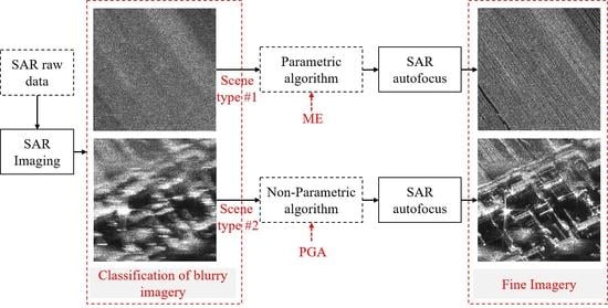
3. Autofocus Approach Based on Blurry Imagery Classification

The flowchart of the proposed autofocus approach based on blurry imagery classification is presented in Figure 3. The first step is to obtain the coarsely focused imagery through SAR imaging processing. The range migration algorithm (RMA) is used as the standard imaging algorithm. After that, we introduce the blurry imagery classification into autofocus processing as a pre-processing, which is different from the traditional autofocus algorithm. The classification of blurry imagery adopts the popular deep learning approach, and the learning network adopts the typical VGGNet [27]. Finally, when the blurry imagery is classified as the scene type #1, the ME algorithm as a parametric method is applied for autofocus processing. On the contrary, if the blurry imagery is classified as the scene type #2, the non-parametric one is adopted (the widely used PGA algorithm is adopted in this article). The proposed approach is detailed in the following.

3.1. Imaging Processing

First, before the classification of blurry imagery, one needs to use the standard imaging algorithm to obtain the coarsely focused imagery, namely, blurry imagery. The standard frequency-domain imaging algorithms mainly include the range-Doppler algorithm and chirp scaling algorithm [32], which are more efficient than the wavenumber-domain algorithms, but they are only suitable for the broadside mode or small squint angle case. The RMA and polar formation algorithm (PFA) belong to the wavenumber-number algorithm [33,34]. They are suitable for the case of large squint angles. Due to the assumption of wavefront curvature, PFA is generally only suitable for small-scene imaging. Therefore, RMA is adopted as the standard imaging algorithm in this article.

It should be pointed out that in the case of large motion error and/or large squint angle, RMA can introduce a serious defocusing in the range direction [33,34]. The influence of range defocusing on blurry image classification is not considered in this article. Therefore, the method proposed in this article is based on the assumption of broadside mode. Futhermore, if the motion error is too large, azimuth defocusing will be too serious, which may lead to wrong classification of blurry imagery. Therefore, this article also needs to use INS/GPS data with certain accuracy to roughly compensate the radar raw data.

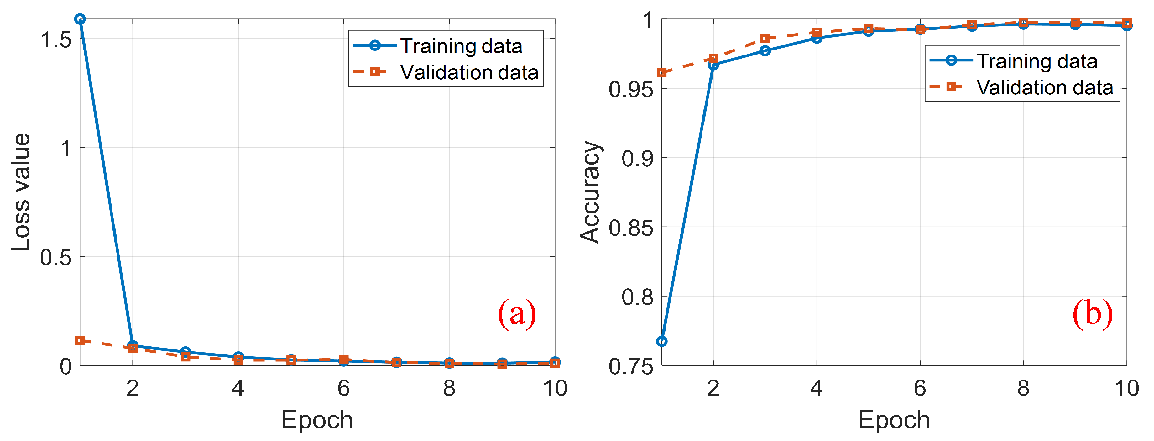
3.2. Blurry Imagery Classification

After applying the standard imaging algorithm (i.e., RMA) to radar raw data, we obtain the blurry imagery. The imaging scene types are divided into two categories, as shown in Figure 4. The purpose of this section is to classify arbitrary blurry imagery accurately to determine to which scene type it belongs. Currently, the deep learning network has been widely used in image classification, so we use this type of approach to classify blurry imagery. Due to the robustness of VGGNet in image classification, VGGNet [27] is used as the learning network. It should be noted that the SAR imagery without autofocus processing usually has different degrees of defocusing and that the defocusing degree is unknown. Therefore, to increase the robustness of the imagery classification learning network, imageries with different defocusing degrees are added to the training data, as shown in Figure 4.

In addition, the imageries used for network training are usually small. For example, the pixels of the imageries for training are 512 × 512, but the actual blurry imagery may have much more pixels (e.g., 8192 × 8192). One solution is to reduce the pixels of the large imagery to the same size as the training imagery by downsampling processing and, then, to input the downsampled imagery into the network for classification. However, because the actual large imageries are very complex, if the downsampled imagery is directly input into the classification network, it may not achieve the classification effect (shown in Section 4). To solve this problem, we divide the large imagery into several small imageries (no overlapping between the imageries) with the same size as the training imageries. After all of the small imageries are input into the classification network, each small imagery corresponds to a classification result. Some small imageries may be classified as scene type #1, while the remaining small imageries are classified as scene type #2. To ensure the robustness of the algorithm, a suitable threshold should be set carefully. If the proportion of all small imageries classified into the scene type #1 exceeds this threshold, this large imagery is regarded as scene type #1. Otherwise, it is considered scene type #2. The discussion of the threshold is presented in Section 4.

3.3. Autofocus Processing

Through the classification of blurry imagery, if it is classified as scene type #1, the parametric method should be applied for autofocus processing. This article uses the image quality optimization algorithm based on the ME criterion. Of course, we can also use other criteria, such as CO or sharpness. The estimation of motion error parameters based on ME criterion can be solved by

$$\stackrel{⌢}{A}=\arg \underset{A}{\min }\{E(G(k,n))\},$$

(1)

where $E\left(·\right)$ donetes the entropy value of the focused imagery $G\left(k,n\right)$. $\left(k,n\right)$ represents the index of the range and azimuth sampling points. A is the parameter set of the motion error to be optimized. The expression of the entropy value is given by

$$E=lnS-\frac{1}{S}\sum _k\sum _n{\left|G\left(k,n\right)\right|}^2·ln{\left|G\left(k,n\right)\right|}^2,$$

(2)

where $S={\displaystyle \sum _k}{\displaystyle \sum _n}{\left|G\left(k,n\right)\right|}^2$.

If it is determined as scene type #2, the widely used PGA algorithm is used in this article. In the standard PGA algorithm, the phase gradient is estimated by the maximum likelihood (ML) estimator, which is given by [35]

$$\Delta \widehat{\dot{}}\phi \left(t_n\right)=arg\left\{\sum _{k=1}^{N}G\left(k,n+1\right)·G^{*}\left(k,n\right)\right\}.$$

(3)

where N denotes the number of seleted range cells.

It should be pointed out that the above blurry imagery classification and autofocus processing are only applicable to spotlight mode and cannot be directly applied to stripmap and other imaging modes. To make the proposed approach suitable for all modes, one can easily introduce the azimuth sub-aperture technique widely used in traditional autofocus processing. For each sub-aperture, we use the processing flowchart shown in Figure 3. After obtaining the motion errors of all sub-apertures, one can integrate all of the azimuth sub-aperture motion errors to obtain the motion error of full-aperture data and finally carry out MoCo and iterative processing.

4. Processing Results of Real Data

Here, we use the processing results of real data to verify the blurry image classification and autofocus processing.

4.1. Classification Verification

Since the imagery before autofocus processing is usually blurry or defocused, we usually classify blurry imageries. Before blurry imagery classification, we need to use a lot of training data to train VGGNet. First, one needs to build the training dataset. Usually, the defocusing degree of blurry imageries is unknown in advance, so we need to generate a large number of blurry images with different defocusing degrees. There are about 7000 imageries for both types of scenes. To achieve this, we use several well-focused SAR imageries to generate imageries with different defocusing degrees by introducing different phase errors in the unfocused domain. It should be noted that the introduced phase error should be a form of higher-order polynomials. However, to simplify the process of blurry imagery generation and considering that the quadratic phase error is the main component, we only introduce a pure quadratic phase error. Figure 4 shows partial datasets of two kinds of scenes with different defocusing degrees. Eighty-five percent of the generated datasets is randomly selected as the training set and fifteen percent is selected as the validation set. The two types of scenes are extracted independently. The imageries in the training and validation dataset are acquired from an X-band radar system working in sliding spotlight mode. The carrier frequency is 8.9 GHz and the resolution is 0.12 m.

It is worth mentioning that, during the production of the training data, we judge the scene type through our experience. For example, no obvious dominant point targets are present in the imageries of the first row in Figure 4, so it is determined to be of scene type #1, while dominant point targets can be seen in the imageries of the second row, so those are regarded to be of scene type #2. For the training of the learning network, the cross-entropy criterion is selected as the loss function and the activation function is the “Relu”. The hyperparameters of the network are that the batch size is 32, the learning rate is 0.0001, the epoch is 10, and the solving algorithm is Adam. Based on VGGNet16, Figure 5 shows the loss function and accuracy varying with the training epoch. The results indicate that the accuracy of the training set can reach 99.5% after 10 epoch training. Finally, we input the validation set into the network for accuracy test, and its accuracy reached 99.7%. We know that different network layers will have different learning results, so we next compare VGGNet13 and VGGNet16.

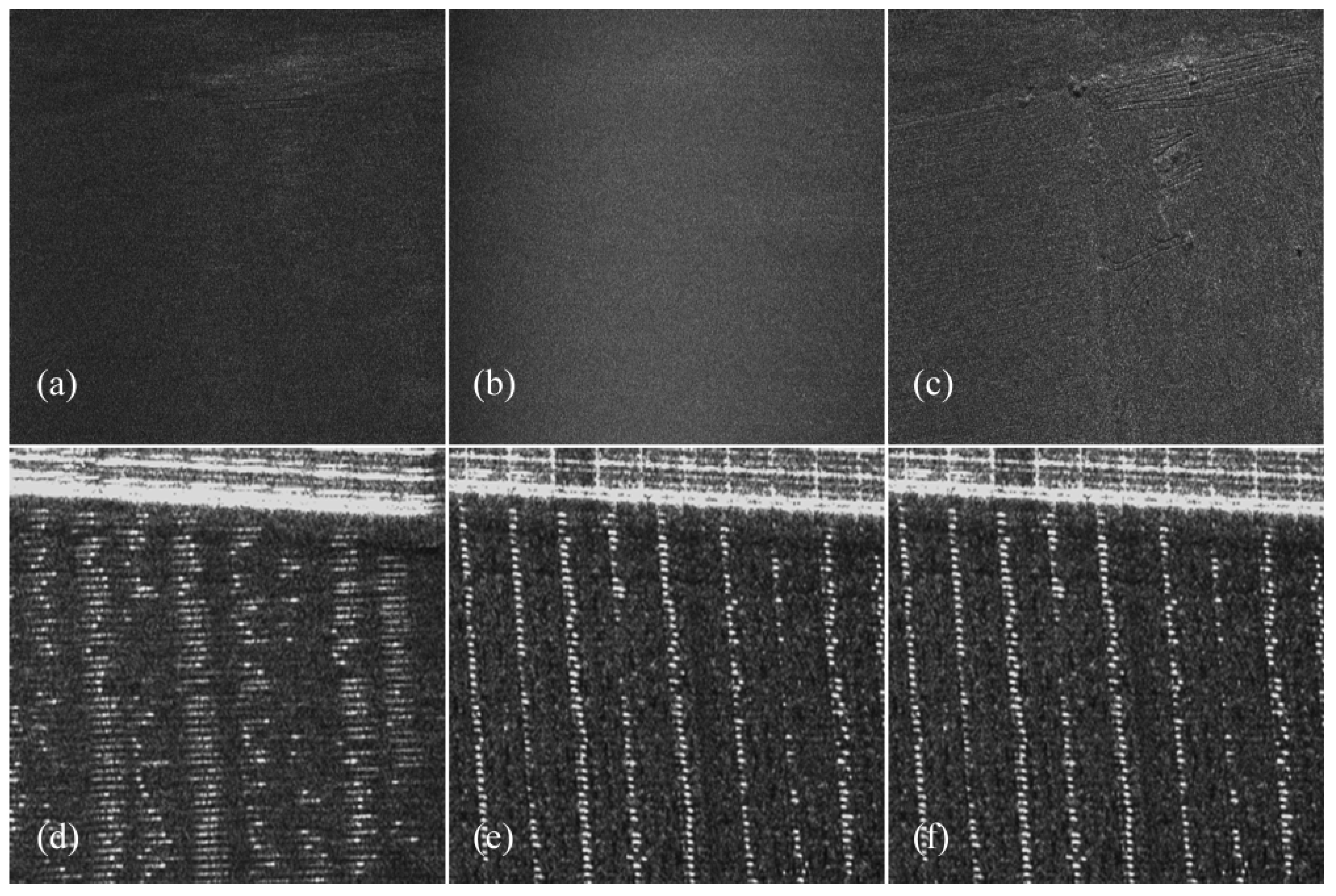
4.2. Autofocus Verification

Additionally, ten different large imageries are used to verify the effectiveness of the proposed approach. VGGNet13 and VGGNet16 are quantatively compared and analyzed. These ten imageries and the imageries in training dateset are acquired from different radar systems. As shown in

Table 2. Classification results of ten large imageries based on VGGNet13. The wrong classification are marked in red.

SAR Imagery	①	②	③	④	⑤	⑥	⑦	⑧	⑨	⑩
Actual Type	#2	#1	#1	#2	#1	#2	#2	#1	#2	#1
Downsampling processing	#1	#1	#1	#1	#1	#1	#2	#1	#2	#1
Ratio of type #1	91/144	144/144	143/144	110/144	7/7	3/7	1/7	139/144	0/7	33/36
Ratio of type #2	53/144	0/144	1/144	34/144	0/7	4/7	6/7	5/144	7/7	3/36
Type by our method (98%)	#2	#1	#1	#2	#1	#2	#2	#2	#2	#2
Type by our method (96%)	#2	#1	#1	#2	#1	#2	#2	#1	#2	#2
Type by our method (94%)	#2	#1	#1	#2	#1	#2	#2	#1	#2	#2

and

Table 3. Classification results of ten large imageries based on VGGNet16. The wrong classification are marked in red.

SAR Imagery	①	②	③	④	⑤	⑥	⑦	⑧	⑨	⑩
Actual Type	#2	#1	#1	#2	#1	#2	#2	#1	#2	#1
Downsampling processing	#1	#1	#1	#1	#1	#1	#2	#1	#2	#1
Ratio of type #1	95/144	143/144	143/144	109/144	7/7	3/7	2/7	139/144	2/7	34/36
Ratio of type #2	49/144	1/144	1/144	35/144	0/7	4/7	5/7	5/144	5/7	2/36
Type by our method (98%)	#2	#1	#1	#2	#1	#2	#2	#2	#2	#2
Type by our method (96%)	#2	#1	#1	#2	#1	#2	#2	#1	#2	#2
Type by our method (94%)	#2	#1	#1	#2	#1	#2	#2	#1	#2	#1

, imageries ⑤, ⑥, ⑦, and ⑨ are obtained by a Ka-band radar operating in sliding spotlight mode. The carrier frequency is 35 GHz, the resolution is 0.2 m, and the imagery size is 3584 × 512. Imageries ①, ②, ③, ④, and ⑧ are obtained by a Ku-band radar operating in spotlight mode. The carrier frequency is 16 GHz, the resolution is 0.1m, and the imagery size is 18,432 × 2048. Imagery ⑩ is obtained by a Ku-band radar operating in stripmap mode. The carrier frequency is 16 GHz, the resolution is 0.6 m, and imagery size of 9557 × 1024.

Their actual type is shown in the second row in Table 2 and Table 3, which can be easily determined by the PGA autofocus results of the ten large imageries. If defocusing occurs in the imagery, it is determined to be of scene type #1. Otherwise, it is of scene type #2. As mentioned previously, because the ten imageries are much larger than the imageries for training, one can resize the large imageries to small imageries directly through the downsampling processing, and the classification results are shown in the third row in Table 2 and Table 3. One can see that imageries ①, ④, and ⑥ are incorrectly classified. Further analysis found that scene type #2 is easily incorrectly classified after downsampling, while the imageries for scene type #1 are all classified correctly. The reason for this is because the downsampling processing may make the dominant point targets in scene type #2 weaker.

Alternatively, we first divide the large imageries into small imageries with a size of 512 × 512. Then, for each large imagery, their small imageries are all put into the network for classification and the output results are statistically analyzed, which are shown in the fourth and fifth rows in Table 2 and Table 3. Using imagery ① as an example and based on VGGNet16, among the 144 small imageries, 95 belong to scene type #1 and 49 belong to scene type #2. As mentioned previously, with a given threshold, we can determine to which category the large imagery belongs. As shown in Table 3, if one sets the threshold as 98% (e.g., 98% of the imageries are judged to be of scene type #1), imageries ⑧ and ⑩ are classified incorrectly (the sixth row in Table 3). If the threshold is 96%, imagery ⑩ is classified incorrectly (the seventh row in Table 3). If the threshold is set as 94%, all ten large imageries are classified correctly (the eighth row in Table 3). Consequently, the threshold should be set carefully. By comparing VGGNet13 with VGGNet16, one can see that when the threshold is set as 94%, imagery ⑩ is wrongly classified by VGGNet13 as shown in Table 2. Therefore, VGGNet16 can achieve a higher accuracy.

After the ten imageries are classified, one knows which type of method should be used for autofocus processing. If it is determined to be of scene type #1, the ME algorithm is applied for autofocus processing. If it is of scene type #2, the PGA algorithm is used. If the threshold is set as 94% and VGGNet16 is adopted, all the large imageries are classified correctly. In this condition, we next compare the autofocus results of the traditional methods and the proposed approach for the ten large imageries. Figure 6 presents the imageries before and after autofocus processing of imageries ⑤ and ⑥. Figure 7 presents partially enlarged imageries of those in Figure 6. From Table 3, the two imageries are classified as scene type #1 and scene type #2 using our approach, respectively. Therefore, if the PGA algorithm is applied to both imageries, the autofocus quality of imagery ⑤ is low. In contrast, the two imageries can be focused well using our approach.

Finally, we quantitatively evaluate the autofocus results based on the entropy criterion for the ten large imageries. The formula of entropy function is shown in (2). The quantitative results are shown in

Table 4. Quality quantitative evaluation of the ten large imageries based on the entropy criterion. The threshold is 94% and VGGNet16 is adopted.

	Entropy Value
SAR imagery	①	②	③	④	⑤	⑥	⑦	⑧	⑨	⑩
No autofocus	12.85	13.44	13.46	13.06	13.04	12.35	12.04	13.46	12.28	12.90
PGA autofocus	12.70	13.46	13.46	12.97	13.06	12.27	11.98	13.46	12.05	12.91
ME autofocus	12.72	13.33	13.35	12.97	13.01	12.29	11.99	13.40	12.14	12.86
Proposed autofocus	12.70	13.33	13.35	12.97	13.01	12.27	11.98	13.40	12.05	12.86

. It is obvious that, for the ten large imageries, the autofocus quality of our approach is no worse than that of the PGA algorithm. It is worth mentioning that, if the ME algorithm is adopted for the ten large imageries, the autofocus quality for all imageries is all high but the efficiency is very low. Therefore, through the preprocessing of blurry imagery classification, we can choose the appropriate autofocus algorithm according to different scene types, avoiding the problem of poor precision in non-parametric autofocus for scene type #1 or avoiding the problem of low efficiency in parametric autofocus methods for scene type #2. The proposed approach combined with blurry imagery classification can achieve better autofocus accuracy and efficiency.

Finally, we dicuss the time-consumption. Compare to the non-parametric and parametric algorithms, the proposed method adds a preprocessing step (i.e., imagery classification), and most of its time-consumption is the training process of the network. Therefore, as long as the network training is completed, the test takes a short time. Using imagery ⑤ as an example, a time-consumption comparison is performed. After testing, the time-consumption of the PGA and ME are 126.9 s and 494.5 s, respectively, while the imagery classification based on VGGNet16 takes only 2.96 s. The experimental environment is as follows: image classification network is based on tensorflow-gpu2.3 version and the used GPU is NVIDIA TITAN RTX. For the ME and PGA methods, MATLAB R2018a based on CPU is adopted and the CPU is Intel Xeon Gold 6234.

5. Conclusions

In this article, a SAR autofocus approach based on blurry imagery classification is proposed. This method embeds blurry image classification as a preprocessing step in traditional autofocus processing. Through this preprocessing, the scene type before autofocus processing can be determined to automatically determine whether to use parametric or non-parametric methods. By using this approach, the capability of the batch processing of airborne SAR data can be improved. The blurry imagery classification is based on a typical VGGNet in a deep learning community. The imagery classification performance based on VGGNet13 and VGGNet16 are compared and indicates that a deep layer could slightly improve the classification accuracy. The effectiveness of the method is verified by the processing results of the real airborne SAR dataset.

Some points needing attention are that this article needs the support of INS/GPS data with certain accuracy to ensure that the azimuth defocusing is not too serious. Besides, the influence of range defocusing on imagery classification is not considered and thus the assumption of broadside mode is adopted in this article, so the imagery classification of largely squint mode needs further study. Deep learning is only introduced into blurry image classification and the traditional autofocus method is still used for radar motion parameter estimation. The radar parameter estimation for SAR autofocus based on deep learning may be an important development direction in the future.

References

1. Moreira, A.; Prats-Iraola, P.; Younis, M.; Krieger, G.; Hajnsek, I.; Papathanassiou, K.P. A tutorial on synthetic aperture radar. IEEE Geosci. Remote Sens. Mag. 2013, 1, 6–43. [Google Scholar] [CrossRef] [Green Version]
2. Yu, H.; Lan, Y.; Yuan, Z.; Xu, J.; Lee, H. Phase Unwrapping in InSAR: A Review. IEEE Geosci. Remote Sens. Mag. 2019, 7, 40–58. [Google Scholar] [CrossRef]
3. Xu, G.; Gao, Y.; Li, J.; Xing, M. InSAR Phase Denoising: A Review of Current Technologies and Future Directions. IEEE Geosci. Remote Sens. Mag. 2020, 8, 64–82. [Google Scholar] [CrossRef] [Green Version]
4. Chen, J.; Zhang, J.; Jin, Y.; Yu, H.; Liang, B.; Yang, D. Real-Time Processing of Spaceborne SAR Data with Nonlinear Trajectory Based on Variable PRF. IEEE Trans. Geosci. Remote. Sens. 2021, 1–12. [Google Scholar] [CrossRef]
5. Xiong, Y.; Liang, B.; Yu, H.; Chen, J.; Jin, Y.; Xing, M. Processing of Bistatic SAR Data With Nonlinear Trajectory Using a Controlled-SVD Algorithm. IEEE J. Sel. Top. Appl. Earth Obs. Remote Sens. 2021, 14, 5750–5759. [Google Scholar] [CrossRef]
6. Chen, X.; Sun, G.C.; Xing, M.; Li, B.; Yang, J.; Bao, Z. Ground Cartesian Back-Projection Algorithm for High Squint Diving TOPS SAR Imaging. IEEE Trans. Geosci. Remote Sens. 2021, 59, 5812–5827. [Google Scholar] [CrossRef]
7. Yi, T.; He, Z.; He, F.; Dong, Z.; Wu, M.; Song, Y. A Compensation Method for Airborne SAR with Varying Accelerated Motion Error. Remote Sens. 2018, 10, 1124. [Google Scholar] [CrossRef] [Green Version]
8. Kirk, J.C. Motion Compensation for Synthetic Aperture Radar. IEEE Trans. Aerosp. Electron. Syst. 1975, AES-11, 338–348. [Google Scholar] [CrossRef]
9. Moreira, J.R. A New Method Of Aircraft Motion Error Extraction From Radar Raw Data For Real Time Motion Compensation. IEEE Trans. Geosci. Remote Sens. 1990, 28, 620–626. [Google Scholar] [CrossRef]
10. Fornaro, G. Trajectory deviations in airborne SAR: Analysis and compensation. IEEE Trans. Aerosp. Electron. Syst. 1999, 35, 997–1009. [Google Scholar] [CrossRef]
11. Lu, Q.; Huang, P.; Gao, Y.; Liu, X. Precise frequency division algorithm for residual aperture-variant motion compensation in synthetic aperture radar. Electron. Lett. 2019, 55, 51–53. [Google Scholar] [CrossRef]
12. Moreira, A.; Huang, Y. Airborne SAR processing of highly squinted data using a chirp scaling approach with integrated motion compensation. IEEE Trans. Geosci. Remote Sens. 1994, 32, 1029–1040. [Google Scholar] [CrossRef]
13. Chen, J.; Xing, M.; Sun, G.; Li, Z. A 2-D Space-Variant Motion Estimation and Compensation Method for Ultrahigh-Resolution Airborne Stepped-Frequency SAR With Long Integration Time. IEEE Trans. Geosci. Remote Sens. 2017, 55, 6390–6401. [Google Scholar] [CrossRef]
14. Chen, J.; Liang, B.; Yang, D.; Zhao, D.; Xing, M.; Sun, G. Two-Step Accuracy Improvement of Motion Compensation for Airborne SAR With Ultrahigh Resolution and Wide Swath. IEEE Trans. Geosci. Remote Sens. 2019, 57, 7148–7160. [Google Scholar] [CrossRef]
15. Xing, M.; Jiang, X.; Wu, R.; Zhou, F.; Bao, Z. Motion Compensation for UAV SAR Based on Raw Radar Data. IEEE Trans. Geosci. Remote Sens. 2009, 47, 2870–2883. [Google Scholar] [CrossRef]
16. Zhang, L.; Qiao, Z.; Xing, M.; Yang, L.; Bao, Z. A Robust Motion Compensation Approach for UAV SAR Imagery. IEEE Trans. Geosci. Remote Sens. 2012, 50, 3202–3218. [Google Scholar] [CrossRef]
17. Li, N.; Niu, S.; Guo, Z.; Liu, Y.; Chen, J. Raw Data-Based Motion Compensation for High-Resolution Sliding Spotlight Synthetic Aperture Radar. Sensors 2018, 18, 842. [Google Scholar] [CrossRef] [Green Version]
18. Wang, G.; Zhang, M.; Huang, Y.; Zhang, L.; Wang, F. Robust Two-Dimensional Spatial-Variant Map-Drift Algorithm for UAV SAR Autofocusing. Remote Sens. 2019, 11, 340. [Google Scholar] [CrossRef] [Green Version]
19. Berizzi, F.; Martorella, M.; Cacciamano, A.; Capria, A. A Contrast-Based Algorithm For Synthetic Range-Profile Motion Compensation. IEEE Trans. Geosci. Remote Sens. 2008, 46, 3053–3062. [Google Scholar] [CrossRef]
20. Xiong, T.; Xing, M.; Wang, Y.; Wang, S.; Sheng, J.; Guo, L. Minimum-Entropy-Based Autofocus Algorithm for SAR Data Using Chebyshev Approximation and Method of Series Reversion, and Its Implementation in a Data Processor. IEEE Trans. Geosci. Remote Sens. 2014, 52, 1719–1728. [Google Scholar] [CrossRef]
21. Yang, L.; Zhou, S.; Zhao, L.; Xing, M. Coherent Auto-Calibration of APE and NsRCM under Fast Back-Projection Image Formation for Airborne SAR Imaging in Highly-Squint Angle. Remote Sens. 2018, 10, 321. [Google Scholar] [CrossRef] [Green Version]
22. Bao, M.; Zhou, S.; Xing, M. Processing Missile-Borne SAR Data by Using Cartesian Factorized Back Projection Algorithm Integrated with Data-Driven Motion Compensation. Remote Sens. 2021, 13, 1462. [Google Scholar] [CrossRef]
23. Wahl, D.E.; Eichel, P.H.; Ghiglia, D.C.; Jakowatz, C.V. Phase gradient autofocus-a robust tool for high resolution SAR phase correction. IEEE Trans. Aerosp. Electron. Syst. 1994, 30, 827–835. [Google Scholar] [CrossRef] [Green Version]
24. Wei, Y.; Yeo, T.S.; Bao, Z. Weighted least-squares estimation of phase errors for SAR/ISAR autofocus. IEEE Trans. Geosci. Remote Sens. 1999, 37, 2487–2494. [Google Scholar] [CrossRef] [Green Version]
25. Zhu, D.; Jiang, R.; Mao, X.; Zhu, Z. Multi-Subaperture PGA for SAR Autofocusing. IEEE Trans. Aerosp. Electron. Syst. 2013, 49, 468–488. [Google Scholar] [CrossRef]
26. Gao, Y.; Yu, W.; Liu, Y.; Wang, R.; Shi, C. Sharpness-Based Autofocusing for Stripmap SAR Using an Adaptive-Order Polynomial Model. IEEE Geosci. Remote Sens. Lett. 2014, 11, 1086–1090. [Google Scholar] [CrossRef]
27. Simonyan, K.; Zisserman, A. Very deep convolutional networks for large-scale image recognition. arXiv 2014, arXiv:1409.1556. [Google Scholar]
28. Wei, S.; Liang, J.; Wang, M.; Zeng, X.; Shi, J.; Zhang, X. CIST: An Improved ISAR Imaging Method Using Convolution Neural Network. Remote Sens. 2020, 12, 2641. [Google Scholar] [CrossRef]
29. Hu, C.; Wang, L.; Li, Z.; Zhu, D. Inverse Synthetic Aperture Radar Imaging Using a Fully Convolutional Neural Network. IEEE Geosci. Remote Sens. Lett. 2020, 17, 1203–1207. [Google Scholar] [CrossRef]
30. Li, R.; Zhang, S.; Zhang, C.; Liu, Y.; Li, X. Deep Learning Approach for Sparse Aperture ISAR Imaging and Autofocusing Based on Complex-Valued ADMM-Net. IEEE Sens. J. 2021, 21, 3437–3451. [Google Scholar] [CrossRef]
31. Gao, J.; Deng, B.; Qin, Y.; Wang, H.; Li, X. Enhanced Radar Imaging Using a Complex-Valued Convolutional Neural Network. IEEE Geosci. Remote Sens. Lett. 2019, 16, 35–39. [Google Scholar] [CrossRef] [Green Version]
32. Cumming, I.G.; Wong, F.H.C. Digital Processing of Synthetic Aperture Radar Data: Algorithms and Implementation; Artech House: Norwood, MA, USA, 2005. [Google Scholar]
33. Mao, X.; Zhu, D. Two-dimensional Autofocus for Spotlight SAR Polar Format Imagery. IEEE Trans. Comput. Imaging 2016, 2, 524–539. [Google Scholar] [CrossRef] [Green Version]
34. Mao, X.; He, X.; Li, D. Knowledge-Aided 2-D Autofocus for Spotlight SAR Range Migration Algorithm Imagery. IEEE Trans. Geosci. Remote Sens. 2018, 56, 5458–5470. [Google Scholar] [CrossRef]
35. Jakowatz, C.V.; Wahl, D.E. Eigenvector method for maximum-likelihood estimation of phase errors in synthetic-aperture-radar imagery. JOSA A 1993, 10, 2539–2546. [Google Scholar] [CrossRef]
Figure 1. Autofocus imageries of scene type #1 by the non-parametric method (a) and parametric method (b).
Remotesensing 13 03872 g001
Figure 2. Autofocus imageries of scene type #2 by the non-parametric method (a) and parametric method (b).
Remotesensing 13 03872 g002
Figure 3. Flowchart of the proposed autofocus approach.
Remotesensing 13 03872 g003
Figure 4. SAR imageries of two kinds of scenes with different defocusing degrees. The first row corresponds to scene type #1, and the second row corresponds to scene type #2. The defocusing degree increases from left to right.
Remotesensing 13 03872 g004
Figure 5. Loss function (a) and accuracy (b) of the training and validation data varying with the epoch.
Remotesensing 13 03872 g005
Figure 6. Autofocus imageries of imageries ⑤ and ⑥. No autofocus (a,d), PGA autofocus (b,e), the proposed approach (c,f).
Remotesensing 13 03872 g006
Figure 7. Enlarged autofocus imageries of imageries ⑤ and ⑥. No autofocus (a,d), PGA autofocus (b,e), the proposed approach (c,f).
Remotesensing 13 03872 g007