Article

Dynamic Assessment of the Impact of Flood Disaster on Economy and Population under Extreme Rainstorm Events

State Key Laboratory of Simulation and Regulation of Water Cycle in River Basin, China Institute of Water Resources and Hydropower Research, Beijing 100038, China
*
Author to whom correspondence should be addressed.
Remote Sens. 2021, 13(19), 3924; https://doi.org/10.3390/rs13193924
Submission received: 3 August 2021 / Revised: 9 September 2021 / Accepted: 27 September 2021 / Published: 30 September 2021
(This article belongs to the Special Issue Remote Sensing in Natural Resource and Water Environment)

Abstract

:
In the context of climate change and rapid urbanization, flood disaster loss caused by extreme rainstorm events is becoming more and more serious. An accurate assessment of flood disaster loss has become a key issue. In this study, extreme rainstorm scenarios with 50- and 100-year return periods based on the Chicago rain pattern were designed. The dynamic change process of flood disaster loss was obtained by using a 1D–2D coupled model, Hazard Rating (HR) method, machine learning, and ArcPy script. The results show that under extreme rainstorm events, the direct economic loss and affected population account for about 3% of the total GDP and 16% of the total population, respectively, and built-up land is the main disaster area. In addition, the initial time and the peak time of flood disaster loss increases with an increasing flood hazard degree and decreases with the increase in the return period. The total loss increases with the increase in the return period, and the unit loss decreases with the increase in the return period. Compared with a static assessment, a dynamic assessment can better reveal the development law of flood disaster loss, which has great significance for flood risk management and the mitigation of flood disaster loss.

1. Introduction

Urban flood disasters, a product of extreme rainfall and the vulnerability and resiliency of the affected area, threaten the security of society and normal development of the economy in cities [1,2,3,4]. According to the statistics about flood disaster loss, China has become one of the most affected countries in the world [5]. In particular, the extreme rainstorm event on July 20 in Zhengzhou, Henan province, caused serious flood disaster loss, which also made the urban flood problem a wide concern to the whole society. Therefore, in order to better deal with urban flooding, several critical questions need to be answered: (1) Under the existing drainage capacity, socio-economic level and underlying surface conditions, how will an extreme rainstorm affect the urban system? (2) What are the distribution characteristics of flood hazard under extreme rainstorm scenarios? (3) What is the development law of flood disasters under different flood hazard degrees? (4) Which measures can we take to reduce the loss as much as possible?
Economic loss and the affected population are the two most important indicators to evaluate the impact of flood disasters on an urban system. Many countries have established their own flood loss estimation models, such as the Hazard United States Multi-Hazards (HAZUS-MH) model developed by FEMA in the United States [6,7], the Flood Loss Estimation Model (FLEMO) [8] and FloodCalc Urban model [9] in Germany, the CLIMADA model in Switzerland [10], Stage–Disaster Curve (SDC) in Italy [11], etc. The assessment methods of the affected population mainly include field research [12] or the disaster footprint, a population database and GIS collaborative technology [13]. The extraction of a disaster footprint includes remote sensing image extraction [14], numerical model simulation [15], and machine learning simulation [16]. A population database includes a demographic database, and a mobile location service provides a dynamic location database [17,18]. Compared to the wealth of methods and available information on flood disaster simulation, fine-resolution data on the spatial distribution of economic and population components are difficult to obtain. This lack of information frequently leads to great uncertainty of flood disaster assessment models in time, space, and across disaster processes [19]. However, the development of big data technology provides the possibility to solve these problems.
In order to obtain fine-resolution economic and population data, some studies have attempted to use Points of Interest (POIs) data to achieve this goal. POIs are open data that are widely used in digital maps such as Google Maps, Baidu Maps, and Amap (Gaode) (the latter two are available only in China) [20]. They generally refer to all geographic objects that can be abstracted as points, especially geographic entities that are closely related to people’s lives, with four aspects of information: name, category, longitude, and latitude. Some studies showed that the degree of POIs agglomeration is related to human production activities, can reflect the current level of population and economic development, and use POIs as an influencing factor to achieve gross domestic product (GDP) and population spatialization [21,22,23]. The fine-resolution spatial information contained in the density layers provided by POIs compensate for the insufficient resolution of existing sources of GDP and population data. Further, the spatialization data of fine-resolution GDP and population data based on POIs can provide supporting data for a flood loss assessment and reduce the uncertainty caused by the coarse resolution of the disaster-bearing body data.
A flood hazard is used to identify the spatial location and intensity of flooding, including the inundation range, inundation depth, flow velocity, and inundation duration, etc. [24,25], and it is also very important for a flood disaster assessment. Hazard calculation methods include the historical disaster method and model simulation method. The model simulation method is the mainstream method for obtaining flood hazard information. Common urban rainstorm models include SWMM, MIKE Urban, InfoWorks ICM, and TEMEMAC-2D, etc. [26,27,28,29]. In this study, the TELEMAC–SWMM coupled model was selected to simulate urban flooding under the following considerations: (1) After decades of development and research, the EXTRAN module and the TELEMAC-2D module have shown strong performance in the fields of one- and two-dimensional hydrodynamics. Their applicability and simulation accuracy in many fields have been extensively verified and recognized [30,31,32]. (2) TELEMAC-2D offers the user a set of FORTRAN subroutines that can be modified to meet the specific requirements of each model, including initial conditions or complex boundary conditions, link-ups with other modeling systems, and the introduction of new functions. (3) The coupled model has a clear physical mechanism, taking into account the hydrological mechanism of surface runoff generation and the hydrodynamic mechanism of pipe network confluence and surface inundation. (4) TELEMAC can output the calculation results of each step, which is helpful for the dynamic assessment of flood disaster loss.
Flood disaster loss assessment methods can be classified into two categories: static methods and dynamic methods [33]. The static methods assess physical damage based on the most severe disaster scenario (e.g., maximum inundation depth) that occurs in an urban system and are mostly used to assess economic loss. The common method is the flood damage curve, which is widely used to assess the impact of flood on buildings and different industries [34,35]. A dynamic assessment emphasizes the impact of flood disaster processes on urban systems. At present, most researches focus on the impact of flood disasters on the population [36], transportation systems [37], and the research methods are mainly based on multi-agent modeling. However, the static assessment of economic loss cannot reflect the dynamic impact of a flood disaster on the economic system, and the multi-agent modeling method is too generalized for the disaster-bearing body and cannot reflect the actual number for the affected population. In particular, the current dynamic assessment method of flood disaster loss lacks a method applicable to both population and economy, and the simulation of flood disaster is mainly based on two-dimensional models, with less consideration for the drainage network, which affects the accuracy of the assessment and leads to an excessive assessment value.
The purpose of this paper is to propose a dynamic assessment method, based on the 1D–2D coupled model, to simulate the development process of flood disasters more realistically, and to evaluate the dynamic impact of flood disaster on the economy and population under extreme rainstorm events. Furthermore, based on big data and machine learning technology, this study solves the problem of poor accuracy in a flood loss assessment caused by the difficulty in obtaining fine-resolution GDP and population data. This study promotes the application of new technologies in the field of urban hydrology and improves the level of the urban natural disaster loss assessment.

2. Materials and Methods

2.1. Study Area

Guangdong Province is the province with the largest permanent population and the most developed economy in China. The Qianshan River Basin is located in the crossover area of Zhongshan city and Zhuhai city in Guangdong Province with an urbanization rate of over 85%, which is an area with dense urban construction. The total catchment area of the basin is approximately 328 km2. In 2020, the permanent population of the basin was 1.0861 million people and the GDP was 16.28 billion USD.
Located in the water-rich region of South China, the basin exists in the subtropical maritime monsoon climate, with abundant rainfall, concentrated rainfall in the flood season, and, mostly, heavy rain of strong intensity and short duration. From 2000 to 2019, the average annual precipitation in the basin was approximately 2216.61 mm (Figure 1b). The rainfall season has a duration of approximately 103 days. The special geographical location and topographical conditions subject the basin to frequent flood disasters caused by typhoon surges, and outer river and local rainfall flooding. In recent years, with the acceleration of urbanization, the surface impervious area has increased, and the loss caused by flood disasters has also increased. According to statistics, in 2018, the direct economic loss caused by flood disasters in Zhongshan City and Zhuhai City was 255.13 million USD and 89.59 million USD, respectively, which were the cities with relatively large economic loss in Guangdong Province. Therefore, it was of certain practical significance to choose the Qianshan river basin as the study area.

2.2. Data Sources

When constructing the urban flood model, five datasets, including pipe network, land use, digital elevation model (DEM), hydrological soil groups, and rainfall, were collected in this study. The pipeline network data were provided by Zhuhai Institute of Urban Planning and Design (Figure 2a). The land use data were obtained though remote sensing interpretation (Figure 2b) and derived from the Gaofen-1 satellite remote sensing image of China Resources Satellite Application Center (http://www.cresda.com/, accessed on 26 September 2021), with a spatial resolution of 16 m. The DEM data were derived from the ASTER GDEM digital elevation data product of the geospatial data cloud (http://slt.gd.gov.cn/, accessed on 26 September 2021), with a spatial resolution of 30 m (Figure 2c). The hydrological soil groups in the study area were divided into four categories: A, B, C, and D. The hydrological soil groups’ data were derived from National Cryosphere Desert Data Center (http://www.ncdc.ac.cn/, accessed on 26 September 2021), with a spatial resolution of 1 km. The design rainstorms were calculated by using the rainstorm intensity equation in Zhuhai issued by the Zhuhai Meteorological Bureau (http://weather.zhuhai.gov.cn/, accessed on 26 September 2021), in which the peak coefficient was 0.4, and the rainfall duration was 120 min:
q = 822.407 1 + 0.776 L n P ( t + 5.000 ) 0.390
where q is design rainstorm intensity, mm/min, P is return period, t is rainfall duration, minute. In this study, extreme rainstorm scenarios were set to 50- and 100-year return periods, and the corresponding rainfall was 209.83 mm and 230.97 mm, respectively.
The curve numbers (CN) and manning coefficients were also key parameters for the urban flood model construction. CN values were determined by the TR55 manual provided by the Natural Resources Conservation Service of the USDA (https://www.nrcs.usda.gov/, accessed on 26 September 2021) as shown in Table 1. The manning coefficients were determined based on the land use types and relevant studies [38] as shown in Table 2.
The POIs data were derived from the Amap Open Platform (https://lbs.amap.com/, accessed on 26 September 2021). There are 20 major categories of POIs on Amap (https://lbs.amap.com/api/webservice/download/, accessed on 26 September 2021). The platform provides an HTTP interface for the search service API and provides a variety of POIs information query capabilities, including keyword, peripheral, polygon searches, and ID query of screening mechanisms. Because the platform has a limit on the number of acquisitions each time (<1000), to prevent missing data in the process of crawling, this study adopted a recursive operation to systematically divide the project area until the number of POIs of each sub-area was less than 1000. Then, the sub-areas were combined to obtain POIs data for the entire project area. In this study, POIs data from 2015 and 2020 were used.
Obtaining fine-resolution GDP and population data required providing training samples for the random forest model. In this study, population data for 2020 were derived from the global high-resolution population denominators project of WorldPop (www.worldpop.org/, accessed on 26 September 2021), with a spatial resolution of 100 m, which has been proven to have very good accuracy [39]. GDP data for 2015 were derived from Resource and Environment Science and Data Center, Institute of Geographic Sciences and Natural Resources Research, Chinese Academy of Sciences (http://www.resdc.cn/, accessed on 26 September 2021), with a spatial resolution of 1 km.

2.3. Methods

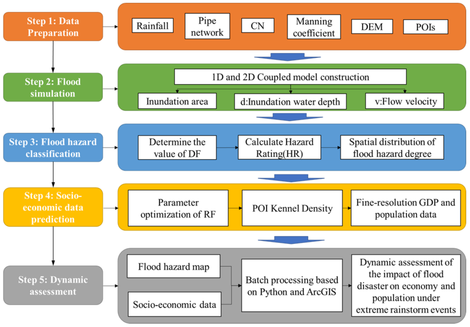
The overall framework of the study is shown in Figure 3, which was divided into five steps: data preparation, flood simulation, flood hazard classification, socio-economic data prediction, and dynamic assessment. In the first step, the design rainstorm, pipe network, land use, CN value, Manning coefficient, and DEM data were collected to provide driving data for the urban flood simulation. The POIs data were used to obtain fine-resolution GDP and population data. The second step was to build a 1D–2D coupled hydrodynamic model to simulate the spatial distribution of the inundation area, inundation depth, and flow velocity. The third step was to use the HR method to obtain the spatial distribution of flood hazard degree. The fourth step was to obtain fine-resolution spatialized data of GDP and population based on the Random Forest (RF) and POIs kernel density data. The fifth step was to realize the dynamic assessment of flood disaster loss based on the ArcPy batch processing script (the tools that needed to be used were Python and ArcGIS).

2.3.1. Principle and Method of Urban Flood Hydrodynamic Model

In this study, a 1D–2D coupled hydrodynamic model was used for urban flood simulation [40]. The coupled mode of this model was loosely coupled. The state variable was used to control the data running order of the EXTRAN and TELEMAC-2D modules. The EXTRAN module is a calculation module developed by the SWMM model for constant flow and unsteady flow, and TELEMAC-2D is a two-dimensional hydrodynamic calculation module. The rainfall runoff calculation adopted the SCS-CN method and was also realized by the TELEMAC module. With water exchange as the link, the water exchange between the one-dimensional pipeline and the two-dimensional surface was realized through the rain grating. The water exchange included the following four situations (Figure 4):
  • h2D < h1D, the node water level was higher than the surface water level, the water flowed from the drainage network to the surface;
  • h1D < Z2D < h2D, the node water level was lower than the surface elevation, the water flowed from the surface to the drainage network;
  • Z2D < h1D < h2D, the node water level was higher than the surface elevation and lower than the surface water level, the water flowed from the surface to the drainage network;
  • Z2D = h1D = h2D, the node water level, surface elevation, and surface water level were all equal, and were in a critical state of water exchange. In this case, it was assumed that no water exchange occurred.
Because, presently, there was no unified calculation method, the usual treatment method of the weir and orifice flow equations was used to calculate the vertical water exchange [40,41]:
The node overflow equation is:
Q n = c 0 A m h 2 g h 1 D h 2 D ,   h 2 D < h 1 D
The node reflux equation is:
Q n = c w h 2 D 2 g h 2 D c 0 A m h 2 g h 2 D h 1 D ,   h 2 D Z 2 D < h 2 D Z 2 D h 1 D < h 2 D
where Qn is exchange flow between one-dimensional drainage pipe network and two-dimensional surface, c0 is orifice outflow coefficient, cw is weir flow coefficient, Amh is the area of the exchange node between the two-dimensional surface and the one-dimensional drainage network, which is the area of the rain grate, w is the width of the top of the weir, that is, the perimeter of the rain grate, g is gravitational constant, h1D is the one-dimensional pipe network node water level, h2D is the two-dimensional surface water level, Z2D is the surface elevation.
The calculation time step size of the coupled model was 1 s, that of the TELEMAC model output was 3 min, and that of the SWMM model output was 15 min.

2.3.2. Flood Hazard Classification Method

A mathematical expression using a method based on empirical data has been widely used to determine flood hazard ratings by the Department for the Environment, Food and Rural Affairs (DEFRA) and the Environment Agency (EA) [42]. This method defines flood hazard rating as a function of flow velocity and water depth. The empirical equation is:
H R = d v + 0.5 + D F
where HR is the flood hazard rating (m2/s), d is the water depth (m), v is the flow velocity (m/s), and DF is the debris factor (m2/s), which can have a value of 0, 0.5, or 1 [43].
Based on the flood hazard rating classification threshold [44], the flood hazard could be divided into four degrees: low, moderate, significant, and extreme.

2.3.3. Spatialization Method of Fine-Resolution GDP and Population

Agriculture, forestry, animal husbandry, and fishery in the primary industry are closely related to farmland, woodland, woodland, and waters in the natural land, respectively. Therefore, in this study, the GDP of the primary industry (GDP1) was spatialized based on different land use types. The calculation equation is as follows:
G D P 1 i = G D P 1 i , j / A 1 j
where GDP1i is the GDP of the primary industry in the ith grid (CNY), GDP1i, j is the total GDP of the jth industry of the primary industry in the ith grid (CNY), A1j is the total area of land use type corresponding to jth industry in the primary industry (km2).
The random forest regression model and POIs data were used to predict GDP of the secondary and tertiary industries (GDP23) in 2020. The GDP23 spatial distribution in 2015 was used to train the random forest regression model, in which the GDP23 spatial distribution was obtained by subtracting the GDP1 from the total GDP in 2015. Seventy percent of the sample data was taken as training sets and the remaining 30% as the test sets. The calculation equations of fine-resolution GDP23 spatial distribution data in 2020 are as follows:
B e s t _ p a r a m = G r i d S e a r c h C V ( R F R ,   p a r a m )
G r i d i _ 30 = R F R _ B e s t _ p a r a m ( P O I _ d e n s i t y i _ 30 )
W i = G r i d i _ 30 i = 1 n G r i d i _ 30
G r i d i _ a c t u a l = W i × T o t a l _ a c t u a l
where RFR is Random Forest Regression model, param is the model parameters to be optimized, GridSearchCV is the grid search algorithm, Best_param is the optimal model parameters, POI_density_30 is the POIs kernel density with a resolution of 30 m in 2020, RFR_ Best_param is the trained random forest regression model, Gridi_30 is the predicted value of the ith grid data, n is the total number of grids in the study area, Total_actual is the actual GDP23 in the study area, Gridi_actual is the actual value of the ith grid.
The calculation method of fine-resolution population data was consistent with that of GDP23. It should be noted that because the population data with a resolution of 100 m could be collected in 2020, the dataset was used to train the random forest model.

2.3.4. Dynamic Assessment Method

The dynamic assessment was realized by the Python program calling the ArcPy batch processing script. The required data included inundation depth, flow velocity, land use, depth–damage curve, and spatial distribution of the disaster-bearing body. A 3-min output time step was set for the inundation depth and flow velocity data. The dynamic assessment process was as follows: based on the inundation depth, flow velocity and land use, the flood hazard rating spatial distribution at each time step was obtained according to Equation (4). Then, the disaster situation of the disaster-bearing body under different flood hazard degrees within each time step was counted. The statistical standard of population was the number, and the statistical standard of GDP was the direct economic loss. The direct economic loss was obtained by multiplying the spatial distribution map of the loss rate with the GDP spatial distribution data. The calculation equation is as follows:
W = i j k A i j η j k
where W is the direct economic loss; i, j, and k are no. of the flood unit, the land use types and inundation depth, respectively; Aij is the GDP of the ith flood unit and jth land use types; ηjk is the loss rate of the kth inundation depth and jth land use types. In this study, the direct economic loss rate was the ratio of direct economic loss to GDP.

3. Results

3.1. Urban Flood Simulation Results

3.1.1. Model Rationality Verification

This study tested the simulation accuracy using the four aspects of waterlogging points (WPs), flood-prone area, runoff coefficient, and flow process to validate the rationality of simulation results to the greatest extent.
The Code for Design of Outdoor Wastewater Engineering (GB50014-2006) (2014 edition) sets the criteria for WPs, namely, the water depth exceeding 0.15 m, the duration exceeding 1 h, and the range exceeding 50 m2. The WPs, a total of 81, were obtained from the Guangdong Research Institute of Water Resources and Hydropower. The datasets are not public; thus, no download link is available. Based on the collected data, 30 m buffer zones were established around the WPs. Through the analysis of the inundation depth in the buffer zones, the number of WPs in different inundation depth ranges was counted to verify the accuracy of the simulation results (Table 3). The results showed that 59 WPs with an accuracy of 72.80% and 61 WPs with an accuracy of 75.31% could be simulated under the 50-year and 100-year return periods, respectively.
The location of flood-prone areas was also obtained from the Guangdong Research Institute of Water Resources and Hydropower. The inundation maps were plotted for two return periods based on the simulation results of the 1D–2D coupled model, as shown in Figure 5a,b. The results showed that the simulated inundation maps could reproduce the flood-prone areas very well.
The runoff coefficients under different return periods were calculated to be 0.66 (50-year) and 0.68 (100-year). According to the Code for Design of Outdoor Wastewater Engineering (GB50014-2006) (2014 edition), the reference value of the runoff coefficient in concentrated urban construction areas should be 0.60~0.70. Therefore, the runoff coefficient was reasonable.
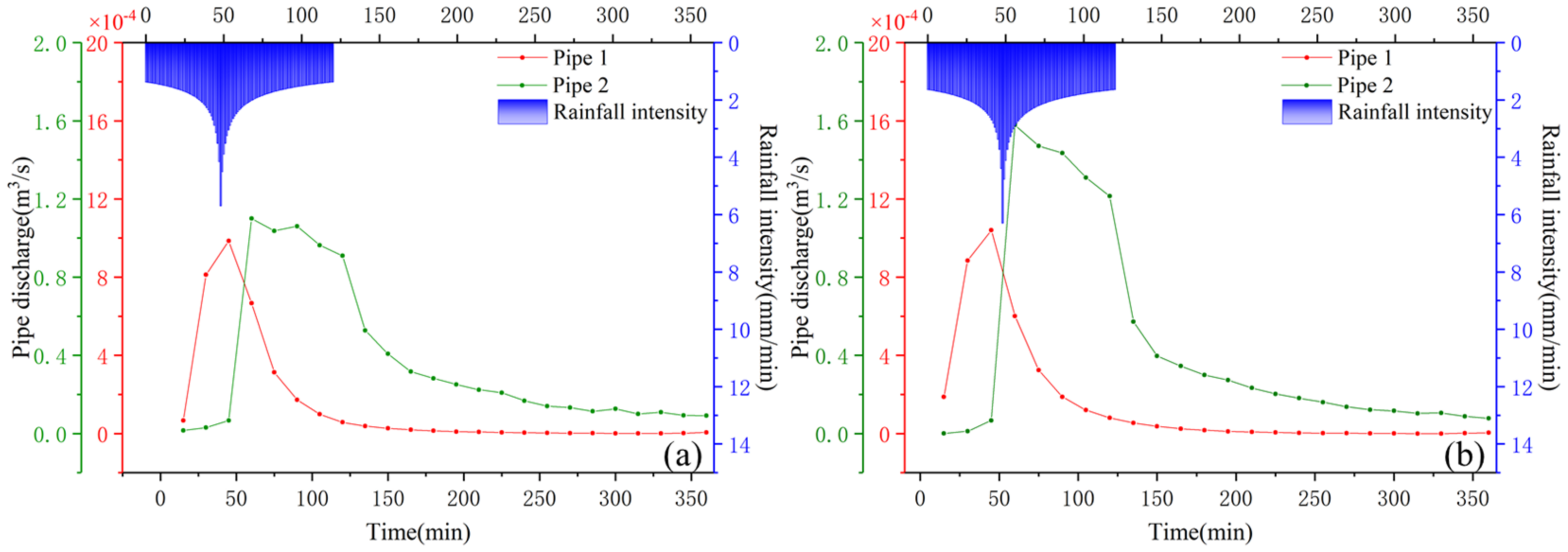
The two river outlets (Figure 2b) located at the Hongwanchong and Qianshan River and two typical pipes (Figure 2a) in the study area were selected. The simulation results of the scalar flowrate time series (Figure 6) at the two basin outlets showed that the model had a high stability, and the flow processes of the two outlets were consistent with other similar studies [45,46]. The typical pipe discharge was also evaluated (Figure 7). The results showed that the pipeline flow process and the rainfall process maintained a high degree of consistency. The maximum pipeline flow coincided with the peak of rainfall. After the rainfall ended, the flow rate decayed very quickly. These results were also consistent with the results of other studies [27,47]. Thus, the simulation results of this model conformed to the basic principles of urban flooding and had a good stability and reliability.

3.1.2. Flood Simulation Results

Figure 8 shows the variation of the flood volume and inundation area over time for different return periods. In this study, the statistical standard of inundation area was the area with inundation depth greater than 0.1 m. The maximum flood volumes were 51,534,080 and 60,597,020 m3 and the maximum inundation areas were 50.95 and 56.87 km2 for the 50- and 100-year return periods, respectively. The change of the flood volume and inundation area showed that, before the rain stopped, the rate of increase was fast to slow; after the rain stopped, the overall trend began to slowly decrease. This change process was consistent with the design rainstorm intensity change process.
The spatial distribution of the inundation depth and flow velocity at the time when the flood volume and inundation area was maximum were plotted based on the simulation results of the urban flood model for two return periods, as shown in Figure 5. The flood-prone areas were mainly urban lands and farmlands. Meanwhile, in the northern part of the basin, the inundation depth and flow velocity were higher, attributed to the topography and the land use type. The surrounding topography not only resulted in a higher flow velocity, but also caused the water to gather, and the lack of an effective drainage channel resulted in more serious waterlogging. The inundation depth and flow velocity were also higher in the river, which reflected that the river channel had a good regulating effect during flood disasters and could effectively discharge flood volume.

3.2. Flood Hazard Classification Results

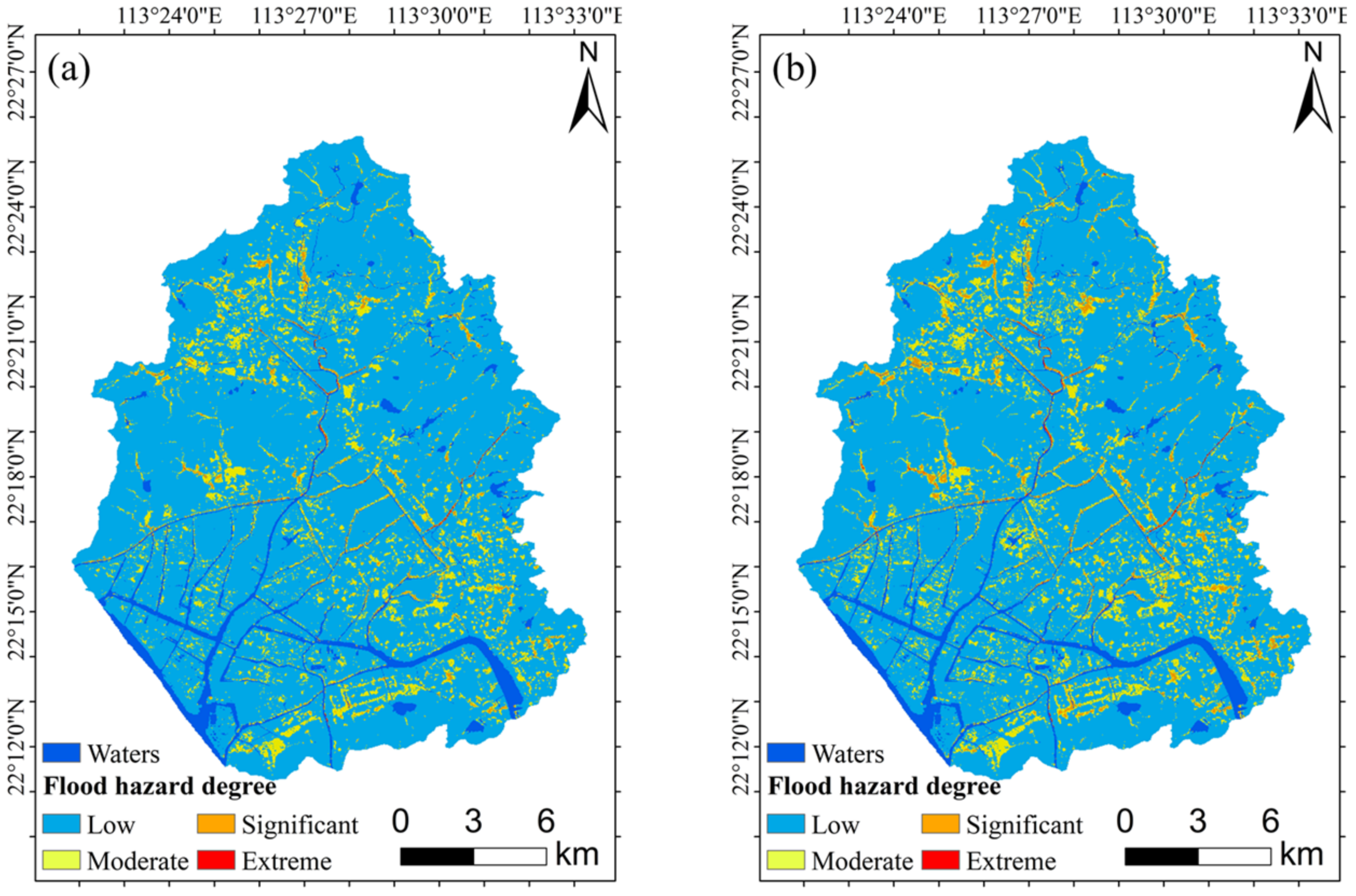
The spatial distribution of flood hazard degrees at the time when the flood volume and inundation area were maximum was plotted, as shown in Figure 9. The results showed that the flood hazard degree in most of the study region was low-degree. The moderate-degree flood hazard was mainly distributed in built-up land, the significant-degree flood hazard was mainly observed in the northwest of the basin, and the extreme-degree flood hazard was mainly observed along the northern and eastern river channels of the basin.
The area of different flood hazard degrees in different land use types for 50- and 100-year return periods was counted (Table 4). The results showed that the area of flood hazard was the largest in built-up land. With the increase in the return period, the area of the low-degree flood hazard area decreased, while the area of the high-degree flood hazard area increased. For the same return period, the area of the extreme-degree flood hazard area increased by the largest proportion. With the return period increased, for the moderate- and significant-degree hazard, the proportion of increased area in farmland was the largest. For the extreme-degree hazard, the proportion of increased area in woodland was the largest. The proportion of increase in the area of significant- and extreme-degree hazard areas was greater than the proportion of increase in moderate-degree areas.

3.3. Flood Disaster Loss Dynamic Assessment

3.3.1. Spatialization of Fine-Resolution GDP and Population Data Based on POIs Kernel Density

Fine-resolution socio-economic data are essential for a flood disaster loss assessment. In this study, 14 categories of POIs closely related to people’s lives were selected to obtain the characteristics of social and economic activities. The number of POIs in 2020 for 14 categories was 100,345. The correlation coefficients between POIs kernel density and GDP and population were calculated (Figure 10a). The results showed that the average correlation coefficients were 0.57 and 0.58, respectively, which belonged to a medium correlation. Based on the random forest regression model, the importance factor of different POIs kernel densities in predicting the spatial distribution of GDP and population was calculated (Figure 10b). The results showed that companies and transportation facilities were the most important in the prediction of the GDP and population, respectively.
In this study, the coefficient of determination (R2) was used for an accuracy evaluation. Table 5 shows the best hyperparameters and the test accuracy of the model. The results showed the accuracy of the training sets to be above 90%, indicating a good fit of the model. For test sets, the accuracy of the GDP and population were 0.6549 and 0.8368, respectively, which could meet the needs of the study.
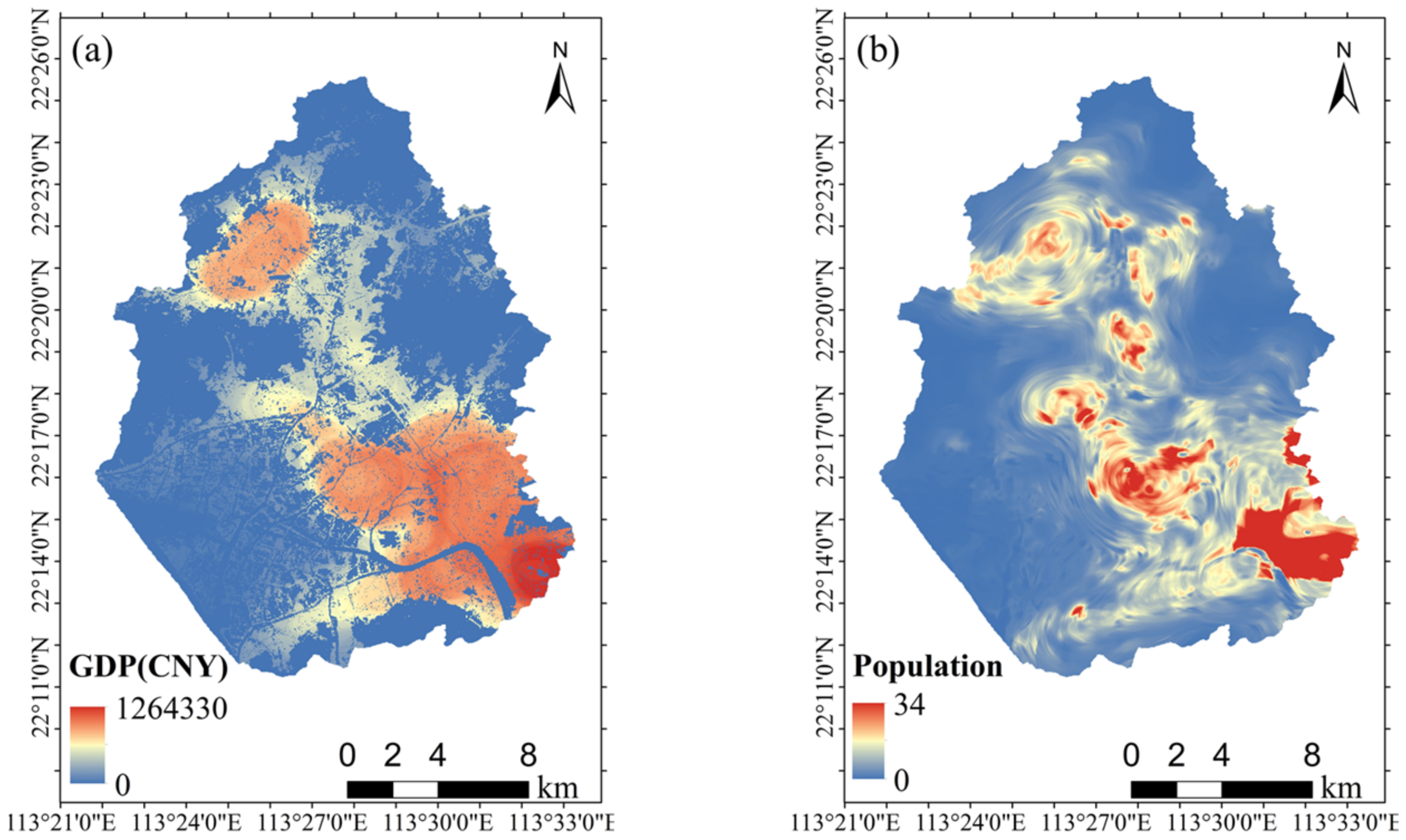
Based on the 14 categories of POIs kernel densities, the trained random forest regression model was applied to the prediction of 30 m fine-resolution GDP and population spatial data from 2020 (Figure 11). The GDP was 105.09 billion CNY and the total population was 1.09 million in 2020. The results showed that the spatial distribution of GDP and population were similar. The southwest, central, and southeast regions of the basin were three core regions. The spatial distribution of the population exhibited the characteristic of a “ripple”, which was related to the independent input variable POIs kernel density.

3.3.2. Dynamic Assessment of the Effect of Flood Disaster on GDP

Referring to relevant literature [48,49], the direct economic loss rate of flood disaster of the different land use types was obtained (Figure 12a). Based on the predicted GDP spatial distribution data of 2020 with a spatial resolution of 30 m, the dynamic change process of direct economic loss was calculated. In addition, based on the flood hazard classification, the direct economic loss in areas of different flood hazard degrees was calculated (Figure 12b).
The change trend of direct economic loss showed that, before the rainfall stopped, the change trend of direct economic loss was consistent with the change trend of the design rainstorm intensity; that is, before the peak rainfall intensity, the increasing speed of direct economic loss was accelerating, and after the peak rain intensity, the increasing speed of direct economic loss was slowing down. After the rainfall stopped, the direct economic loss immediately began to decrease, which was consistent with the changing trend of flood volume and inundation area.
The maximum direct economic losses were 2.77 and 3.18 billion CNY for the 50- and 100-year rainstorm return periods, respectively, with ratio increases of 14.84% of the 100-year return over the 50-year return. The direct economic loss under different hazard degrees at the same time was also evaluated. For the 50-year return period, the direct economic loss from the low-, moderate-, significant-, and extreme-degree hazard areas were 1.00, 1.33, 0.39, and 0.37 billion CNY, respectively. For the 100-year return period, the direct economic loss was 0.99, 1.51, 0.60, and 0.62 billion CNY, respectively, with ratio increases of −0.51%, 13.45%, 53.55%, and 69.37% of the 100-year return over the 50-year return. Therefore, the direct economic loss was mainly distributed in the low- and moderate-degree hazard areas. However, with the increase in the return period, the increase in the direct economic loss in both the significant- and extreme-degree hazard areas was much higher than that in the low- and moderate-degree hazard areas, and the increase in the significant-degree hazard area was the largest.
The maximum direct economic loss under different flood hazard degrees was evaluated. The results showed that, for the 50-year return period, the peak loss from the low-, moderate-, significant-, and extreme-degree hazard areas was 1.10, 1.51, 0.67, and 0.09 billion CNY, respectively, and for the 100-year return period, the peak loss was 1.07, 1.33, 0.45, and 0.07 billion CNY, respectively, with ratio increases of 3.31%, 13.41%, 47.74%, and 23.71% of 100-year return over 50-year return data. The largest increase was also in the significant hazard degree.

3.3.3. Dynamic Assessment of the Effect of Flood Disaster on Population

Based on the predicted population spatial distribution data for 2020 with a spatial resolution of 30 m, the dynamic change process of the number of flood-affected population was counted (Figure 13). In addition, based on the flood hazard classification, the number of the flood-affected population in areas of different flood hazard degrees was evaluated. Relevant literature [44] described the meaning of different flood hazard degrees, in which the impact on people’s activities started from the moderate hazard degree. Therefore, in this study, the population in the low hazard degree was defined as the potential flood-affected population, and the population in other hazard degrees was defined as the flood-affected population.
The trend of the dynamic change of the potential flood-affected population varied from “unchanged” to “decreasing rapidly” to “increasing slowly”, and that of the flood-affected population varied from “unchanged” to “increasing rapidly” to “decreasing slowly”. The maximum flood-affected population occurred in the 120th min, which was immediately after the rainfall stopped. At that moment, the number of flood-affected people was 160,303 and 189,824 in the 50- and 100-year rainstorm return periods, respectively, with a rate increase of 18.42%. The flood-affected population under different hazard degrees at that time was evaluated. For the 50-year return period, the affected number of people from the moderate-, significant-, and extreme-degree hazard areas were 136,231, 22,859, and 1212, respectively. For the 100-year return period, the affected number was 152,211, 35,533, and 2080, respectively, with ratio increases of 10.50%, 35.67%, and 41.74% of the 100-year over 50-year return periods. Therefore, the flood-affected population was mainly distributed in the moderate-degree hazard areas. However, with the increase in the return period, the increase in the proportion of the flood-affected population in both the significant- and extreme-degree hazard areas was higher than that in the moderate-degree hazard areas, and the increase in the proportion of the extreme-degree hazard areas was the largest.
The peak flood-affected population under different flood hazard degrees was also evaluated. The results showed that for the 50-year return period, the peak flood-affected the population from the moderate-, significant-, and extreme-degree hazard areas was 136,231, 23,075, and 2197, respectively. For the 100-year return period, the peak flood-affected population was 152,211, 36,242, and 2785, respectively, with ratio increases of 11.73%, 57.06%, and 26.74% of the 100-year over 50-year return periods. The largest increase was in the significant hazard degree.

4. Discussion

4.1. The Development Rules of Flood Disaster Loss under Different Flood Hazards

The initial occurrence time of flood disaster loss for different flood hazard degree areas was calculated (Table 6). The results showed that the initial time of flood disaster loss increased with the increase in flood hazard degree and decreased with the increase in flood return period. This was because the higher the flood hazard degree, the greater the inundation depth and flow velocity, which requires a greater rainfall and rainfall intensity. Therefore, the occurrence time for flood disaster was relatively lag. The greater the return period, the greater the rainfall and rainfall intensity, which would also lead to the early occurrence of a high-degree flood hazard.
The statistical results of the peak occurrence time of flood disaster loss under different flood hazard degree areas (Table 7) showed that the development law was consistent with the initial occurrence time of flood disaster loss; that is, it increased with the increase in the flood hazard degree and decreased with the increase in the flood return period. Meanwhile, the maximum direct economic loss occurred, obviously, later than the maximum moment of the affected population in the significant-degree flood hazard area. However, the maximum direct economic loss occurred obviously earlier than the maximum moment of the affected population in the extreme-degree flood hazard area.
The flood disaster loss under different flood hazard degrees at peak time was calculated, including the total loss and unit loss (Table 8). In terms of the total loss, the number of the flood-affected population was the largest in the moderate-degree hazard areas, and the direct economic loss was the largest in the low-degree hazard areas. This was because the lower the flood hazard degree, the larger the area affected, and the total flood disaster loss was larger. In terms of the loss per unit area, the maximum loss per unit area of the GDP and population was in the extreme- and significant-degree hazard areas, respectively. Overall, in moderate-, significant- and extreme-degree hazard areas, the total loss increased with the increase in the return period, and the unit loss decreased with the increase in the return period. Although the extreme-degree hazard areas would have a more serious effect on the disaster-bearing body, the total loss was not the highest because of the small area of the extreme-degree hazard areas. Meanwhile, limited by the spatial distribution of the disaster-bearing body, the loss per unit area of the extreme-degree hazard areas was not necessarily the largest. This enabled us to understand that the flood disaster loss was not necessarily large in the region with a higher degree flood hazard, which was related to the size of the hazard areas and the spatial distribution of the disaster-bearing body.

4.2. Suggestions on Measures to Reduce Flood Disaster Loss

In order to reduce urban flood disaster loss and maintain the urban structure and function, these must be achieved by taking engineering and non-engineering measures to resist, absorb, and adapt to flood risks [50].
Engineering measures: These mainly rely on the construction of high-standard urban drainage systems and flood control systems, the construction content mainly includes widening river courses, adding municipal drainage pipes, drainage pump stations, levees, sluice, reservoirs, increasing the diameter of drainage pipes, etc. In addition, sponge cities can be built to improve the urban control ability of storm runoff [51].
Non-engineering measures: These mainly include a strengthening risk management, improving forecasting and early warning capabilities, improving flood control standards and related regulations, raising public awareness, building smart water services [52] and smart cities [53], and purchasing urban flood insurance [54], etc.

4.3. Uncertainty in Research

4.3.1. The Uncertainty of Flood Simulation

In this study, the DEM of 30 m resolution was adopted. This DEM resolution seemed pretty coarse for urban modeling. It was undeniable that this would affect the accuracy of the urban flood simulation. The purpose of this research was to propose a dynamic assessment method to grasp the development characteristics of flood disaster losses during the occurrence of floods, and to guide the formulation of disaster prevention and mitigation measures. Therefore, there were higher requirements for the timeliness of the model. At present, most of the research on urban flood disaster assessment is a static assessment, and the demand for timeliness of the model is low, so fine-resolution DEM data can be used to obtain a higher assessment accuracy. However, in this study, in order to make the assessment objects more complete, the basin scale was selected. The basin included not only urban areas, but also farmland, woodland, and grassland. If fine-resolution DEM data were used, the computational grid would increase geometrically, which would have a greater impact on the timeliness of the model. Therefore, this research had to improve the timeliness of calculation by using lower resolution DEM data. Meanwhile, due to the lack of spatialized economic and population data that matched the fine-resolution DEM data, the impact on the evaluation results was within an acceptable range. Future studies should try to adopt GPU acceleration technology and use different resolution networks for different areas. For example, high-resolution DEMs are used in urban areas. Because of the small spatial differences in woodland, grassland, and farmland, low-resolution networks can be used.
Moreover, this study did not further classify urban areas, such as industrial areas, commercial areas, and residential areas (low residential, medium–low residential, high–low residential), etc. The CN value and Manning coefficient were not determined according to different categories, which would also increase the uncertainty of the simulation results. This was mainly due to the low availability of the above data and the lack of corresponding disaster loss curves in this study area. Future studies should strengthen the collection of data, such as the vector outlines and attributes of different buildings, and the disaster loss curves of different building types, and combine the location information of different services provided by POI to refine the urban area. Additionally, they should consider the difference in disaster loss of different building types to improve the accuracy of the urban flood disaster loss assessment.

4.3.2. The Uncertainty of Flood Disaster Loss Assessment

In terms of the flood disaster loss assessment, this study assessed the flood disaster loss under two design rainstorms, and the accumulated rainfall amount was 209.83 mm and 230.97 mm for the 50- and 100-year return periods, respectively, and the rainfall duration was 2 h, both of which belonged to the extreme rainstorm. The disaster loss brought by such a design rainstorm scenario was undoubtedly huge. According to the existing data, for the rainstorm of more than 200mm, its rainfall duration was usually greater than 24 h, so the simulation results lacked comparison data. However, an extreme rainstorm event recently occurred in Zhengzhou, Henan Province, with the one-hour rainfall reaching 201.9 mm, which was similar to the extreme rainstorm scenario set in this study. Take the “7.20” extreme rainstorm event in Henan province as an example, according to preliminary statistics, the Zhengzhou extreme rainstorm led to direct economic loss of 65.5 billion CNY, accounting for 5.46% of the total GDP, and emergency relocation of 395,989 people, accounting for 3.83% of the total population. In this study, for the 50- and 100-year return periods, the direct economic loss accounted for 2.63% and 3.02% of the total GDP, and the affected population accounted for 14.76% and 17.49% of the total population, respectively. The results showed that the proportion of direct economic loss in GDP in the study area was slightly less than the 7.20 rainstorm event in Zhengzhou, and the statistical value of the affected population was greater than the 7.20 rainstorm event in Zhengzhou. The less direct economic loss may have been due to the large area of farmland and forestry in the study area, which led to a lower economic level in this area than in Zhengzhou. The large differences in the affected population may have been due to different statistical standards. In this study, all people in the flood area were considered as the affected population. However, different from property distribution, people would adopt different risk aversion strategies, so the actual statistical results would be smaller than the simulation results.

4.3.3. The Uncertainty of Machine Learning

When using the random forest model to predict the spatial distribution of GDP and population, the correlation coefficients between POIs kernel density and GDP and population were the same, but the predicted results were quite different, in which the R2 of GDP and population was 0.6549 and 0.8368, respectively. From the perspective of the R2 value, the results of this study were consistent with those of related studies [21,23,55,56,57]. The main reason for the difference was that R2 was chosen as the evaluation index. Some studies have shown that the value of R2 was strongly affected by the number of samples [58]. The number of training sets used for the GDP and population in this study was quite different. The spatial resolution of the GDP was 1 km, while the spatial resolution of the population was 100 m.

4.4. Future Studies

Four areas for future research consist of the following:
  • The prediction accuracy of the GDP spatial distribution data was 65%. Future studies should try some methods to solve this problem, such as adding training samples, increasing the type of input variables, or comparing the accuracy of different machine learning methods;
  • Machine learning algorithms have been widely used, but they are rarely used in the field of urban hydrology. This study attempted to use machine learning algorithms to obtain fine-resolution socio-economic data, which provided data for a flood disaster loss assessment. Future studies should explore the application of machine learning algorithms in the field of urban hydrology such as obtaining flood inundation maps based on machine learning to improve the timeliness of flood simulations;
  • The results of this study showed that the return period had an effect on the initial time and peak occurrence time of the flood disaster. However, only two rainstorm situations were set in this study, resulting in limitations in the conclusions. Future studies will construct a variety of rainstorm situations by setting different peak coefficients, rainfall durations, and return periods to investigate the dynamic assessment of flood disaster loss under various rainstorm designs, and to identify the influence of rainfall characteristics on the development process of flood disaster loss;
  • Different from property distribution, people should adopt different risk avoidance strategies, which would lead to a great uncertainty when using a static assessment method to calculate the number of the affected population. Therefore, future research should combine the multi-agent model to study the impact of different risk avoidance strategies on the number of the affected population and improve the accuracy of the assessment model.

5. Conclusions

Based on a numerical simulation, big data, machine learning, and ArcPy batch processing scripts, this research evaluated the dynamic impact of flood disasters on the economy and population under extreme rain conditions. The main conclusions were as follows:
  • Under extreme rainstorm conditions, flood disaster had a serious impact on economy and population. For the 50- and 100-year return periods, the maximum direct economic loss was 2.77 billion CNY and 3.18 billion CNY, respectively, accounting for 2.63% and 3.02% of the total GDP, respectively. The affected population was 160,303 and 189,924, respectively, accounting for 14.76% and 17.49% of the total population, respectively;
  • The higher degree flood hazard areas were mainly distributed on built-up land. Moreover, with the increase in the return period, the higher degree flood hazard areas had a greater proportion of increase;
  • In terms of the occurrence time of flood disaster loss, the initial time and the peak time of flood disaster loss increased with an increasing flood hazard degree and decreased with the increase in the return period. In terms of the flood disaster loss, in moderate-, significant-, and extreme-degree hazard areas, the total loss increased with the increase in the return period, and the unit loss decreased with the increase in the return period;
  • Under the design rainstorm scenario of the Chicago rain pattern, the process of flood loss development had a stage of rapid increase.
In the future, we could adopt different disaster prevention and mitigation measures according to the development rules of flood disaster loss in different flood hazard areas, such as improving the urban flood control and drainage standards, building sponge cities, providing public awareness, increasing the extreme rainstorm warning and buying urban flood insurance, etc., so as to better deal with the climate risk brought by extreme rainstorm events.

Author Contributions

Conceptualization, X.S., W.S., J.L., Y.J., and K.W.; methodology, X.S., W.S., and J.L.; software, X.S. and K.W.; validation, X.S. and K.W.; formal analysis, X.S.; investigation, X.S.; resources, W.S., J.L., and Y.J.; data curation, X.S. and W.S.; writing—original draft preparation, X.S.; writing—review and editing, X.S., W.S., and J.L.; visualization, X.S., W.S., and K.W.; supervision, J.L. and Y.J.; project administration, W.S. All authors have read and agreed to the published version of the manuscript.

Funding

This research was funded by the Chinese National Key Research and Development Program, grant number 2018YFC1508203; National Natural Science Foundation of China, grant numbers 51979285, 51739011 and 51879274; Research Fund of the China Institute of Water Resources and Hydropower Research, grant numbers WR0145B502016 and 2017ZY02.

Institutional Review Board Statement

Not applicable.

Informed Consent Statement

Not applicable.

Data Availability Statement

The data are currently unavailable online due to an embargo, but are available by an email arrangement.

Acknowledgments

Thanks are given to the anonymous reviewers and editors for their constructive comments.

Conflicts of Interest

The authors declare no conflict of interest.

References

  1. Wu, Z.; Shen, Y.; Wang, H.; Wu, M. Urban flood disaster risk evaluation based on ontology and Bayesian Network. J. Hydrol. 2020, 583, 124596. [Google Scholar] [CrossRef]
  2. Luo, P.; Mu, D.; Xue, H.; Ngo-Duc, T.; Dang-Dinh, K.; Takara, K.; Nover, D.; Schladow, G. Flood inundation assessment for the Hanoi Central Area, Vietnam under historical and extreme rainfall conditions. Sci. Rep. 2018, 8, 12623. [Google Scholar] [CrossRef]
  3. Mu, D.; Luo, P.; Lyu, J.; Zhou, M.; Huo, A.; Duan, W.; Nover, D.; He, B.; Zhao, X. Impact of temporal rainfall patterns on flash floods in Hue City, Vietnam. J. Flood Risk Manag. 2020, 14, e12668. [Google Scholar] [CrossRef]
  4. Chao, L.; Zhang, K.; Li, Z.; Wang, J.; Yao, C.; Li, Q. Applicability assessment of the CASCade Two Dimensional SEDiment (CASC2D-SED) distributed hydrological model for flood forecasting across four typical medium and small watersheds in China. J. Flood Risk Manag. 2019, 12, e12518. [Google Scholar] [CrossRef] [Green Version]
  5. Cai, T.; Li, X.; Ding, X.; Wang, J.; Zhan, J. Flood risk assessment based on hydrodynamic model and fuzzy comprehensive evaluation with GIS technique. Int. J. Disaster Risk Reduct. 2019, 35, 101077. [Google Scholar] [CrossRef]
  6. Scawthorn, C.; Blais, N.; Seligson, H.; Tate, E.; Mifflin, E.; Thomas, W.; Murphy, J.; Jones, C. HAZUS-MH flood loss estimation methodology. I: Overview and flood hazard characterization. Nat. Hazards Rev. 2006, 7, 60–71. [Google Scholar] [CrossRef]
  7. Scawthorn, C.; Flores, P.; Blais, N.; Seligson, H.; Tate, E.; Chang, S.; Mifflin, E.; Thomas, W.; Murphy, J.; Jones, C. HAZUS-MH flood loss estimation methodology. II. Damage and loss assessment. Nat. Hazards Rev. 2006, 7, 72–81. [Google Scholar] [CrossRef]
  8. Thieken, A.; Olschewski, A.; Kreibich, H.; Kobsch, S.; Merz, B. Development and evaluation of FLEMOps–a new Flood Loss Estimation MOdel for the private sector. WIT Trans. Ecol. Environ. 2008, 118, 315–324. [Google Scholar] [CrossRef]
  9. Meyer, V.; Scheuer, S.; Haase, D. A multicriteria approach for flood risk mapping exemplified at the Mulde river, Germany. Nat. Hazards 2009, 48, 17–39. [Google Scholar] [CrossRef]
  10. Aznar-Siguan, G.; Bresch, D.N. CLIMADA v1: A global weather and climate risk assessment platform. Geosci. Model Dev. 2019, 12, 3085–3097. [Google Scholar] [CrossRef] [Green Version]
  11. Amadio, M.; Mysiak, J.; Carrera, L.; Koks, E. Improving flood damage assessment models in Italy. Nat. Hazards 2016, 82, 2075–2088. [Google Scholar] [CrossRef] [Green Version]
  12. Husby, T.G.; de Groot, H.L.; Hofkes, M.W.; Dröes, M.I. Do floods have permanent effects? Evidence from the Netherlands. J. Reg. Sci. 2014, 54, 355–377. [Google Scholar] [CrossRef]
  13. Guha-Sapir, D.; Rodriguez-Llanes, J.M.; Jakubicka, T. Using disaster footprints, population databases and GIS to overcome persistent problems for human impact assessment in flood events. Nat. Hazards 2011, 58, 845–852. [Google Scholar] [CrossRef] [Green Version]
  14. Feng, Q.; Liu, J.; Gong, J. Urban flood mapping based on unmanned aerial vehicle remote sensing and random forest classifier—A case of Yuyao, China. Water 2015, 7, 1437–1455. [Google Scholar] [CrossRef]
  15. Smith, A.; Bates, P.D.; Wing, O.; Sampson, C.; Quinn, N.; Neal, J. New estimates of flood exposure in developing countries using high-resolution population data. Nat. Commun. 2019, 10, 1–7. [Google Scholar] [CrossRef] [PubMed] [Green Version]
  16. Mosavi, A.; Ozturk, P.; Chau, K.-w. Flood prediction using machine learning models: Literature review. Water 2018, 10, 1536. [Google Scholar] [CrossRef] [Green Version]
  17. Zhang, S.; Zhang, W.; Wang, Y.; Zhao, X.; Song, P.; Tian, G.; Mayer, A.L. Comparing human activity density and green space supply using the Baidu Heat Map in Zhengzhou, China. Sustainability 2020, 12, 7075. [Google Scholar] [CrossRef]
  18. Weiwei, S.; Xin, S.; Jie, L.; Jiahong, L.; Zhiyong, Y.; Yongqiang, C.; Zhaohui, Y.; Kaibo, W. The application of big data in the analysis of the impact of urban floods: A case study of Qianshan River Basin. J. Phys. Conf. Ser. 2021, 1955, 012061. [Google Scholar] [CrossRef]
  19. Merz, B.; Kreibich, H.; Schwarze, R.; Thieken, A. Review article ”Assessment of economic flood damage”. Nat. Hazard Earth Sys. 2010, 10, 1697–1724. [Google Scholar] [CrossRef]
  20. Huang, W. Macro Analysis of Urban Structure Based on Point of Interest. In Proceedings of the 2016 6th International Conference on Mechatronics, Computer and Education Informationization (MCEI 2016), Shenyang, China, 11–13 November 2016; pp. 928–932. [Google Scholar]
  21. Li, K.; Chen, Y.; Li, Y. The random forest-based method of fine-resolution population spatialization by using the international space station nighttime photography and social sensing data. Remote Sens. 2018, 10, 1650. [Google Scholar] [CrossRef] [Green Version]
  22. Wang, Y.; Huang, C.; Zhao, M.; Hou, J.; Zhang, Y.; Gu, J. Mapping the Population Density in Mainland China Using NPP/VIIRS and Points-Of-Interest Data Based on a Random Forests Model. Remote Sens. 2020, 12, 3645. [Google Scholar] [CrossRef]
  23. Zhang, A.; Pan, Y.; Ming, Y.; Wang, J. Research of GDP Spatialization based on Multi-source Information Coupling: A Case Study in Beijing. Remote Sens. Technol. Appl. 2021, 36, 463–472. [Google Scholar] [CrossRef]
  24. Apel, H.; Aronica, G.; Kreibich, H.; Thieken, A. Flood risk analyses—how detailed do we need to be? Nat. Hazards 2009, 49, 79–98. [Google Scholar] [CrossRef]
  25. Zhou, Q.; Mikkelsen, P.S.; Halsnæs, K.; Arnbjerg-Nielsen, K. Framework for economic pluvial flood risk assessment considering climate change effects and adaptation benefits. J. Hydrol. 2012, 414, 539–549. [Google Scholar] [CrossRef]
  26. Mei, C.; Liu, J.; Wang, H.; Yang, Z.; Ding, X.; Shao, W. Integrated assessments of green infrastructure for flood mitigation to support robust decision-making for sponge city construction in an urbanized watershed. Sci. Total Environ. 2018, 639, 1394–1407. [Google Scholar] [CrossRef]
  27. Bisht, D.S.; Chatterjee, C.; Kalakoti, S.; Upadhyay, P.; Sahoo, M.; Panda, A. Modeling urban floods and drainage using SWMM and MIKE URBAN: A case study. Nat. Hazards 2016, 84, 749–776. [Google Scholar] [CrossRef]
  28. Sheng, J.G.; Dan, Y.D.; Liu, C.S.; Ma, L.M. Study of Simulation in Storm Sewer System of Zhenjiang Urban by Infoworks ICM Model. In Applied Mechanics and Materials; Trans Tech Publications Ltd.: Bäch, Switzerland, 2012; pp. 683–686. [Google Scholar]
  29. Mei, C.; Liu, J.; Wang, H.; Li, Z.; Yang, Z.; Shao, W.; Ding, X.; Weng, B.; Yu, Y.; Yan, D. Urban flood inundation and damage assessment based on numerical simulations of design rainstorms with different characteristics. Sci. China Technol. Sci. 2020, 63, 2292–2304. [Google Scholar] [CrossRef]
  30. Jahanbazi, M.; Egger, U. Application and comparison of two different dual drainage models to assess urban flooding. Urban Water J. 2014, 11, 584–595. [Google Scholar] [CrossRef]
  31. Li, Z.; Liu, J.; Mei, C.; Shao, W.; Wang, H.; Yan, D. Comparative Analysis of Building Representations in TELEMAC-2D for Flood Inundation in Idealized Urban Districts. Water 2019, 11, 1840. [Google Scholar] [CrossRef] [Green Version]
  32. Zhu, J.; Dai, Q.; Deng, Y.; Zhang, A.; Zhang, Y.; Zhang, S. Indirect damage of urban flooding: Investigation of flood-induced traffic congestion using dynamic modeling. Water 2018, 10, 622. [Google Scholar] [CrossRef] [Green Version]
  33. He, J.; Qiang, Y.; Luo, H.; Zhou, S.; Zhang, L. A stress test of urban system flooding upon extreme rainstorms in Hong Kong. J. Hydrol. 2021, 597, 125713. [Google Scholar] [CrossRef]
  34. Romali, N.S.; Yusop, Z.; Ismail, Z. Flood damage assessment: A review of flood stage–damage function curve. In ISFRAM 2014; Springer: Singapore, 2015; pp. 147–159. [Google Scholar] [CrossRef] [Green Version]
  35. Romali, N.S.; Yusop, Z. Flood damage and risk assessment for urban area in Malaysia. Hydrol. Res. 2021, 52, 142–159. [Google Scholar] [CrossRef]
  36. Li, W.; Guo, X.; Mao, X.; Xiao, D.; Lai, W.; Wang, H. The dynamic population risk assessment model for rainstorm-flood utilization multi-agent. J. Catastrophol. 2015, 30, 80–87. [Google Scholar]
  37. Pyatkova, K.; Chen, A.S.; Butler, D.; Vojinović, Z.; Djordjević, S. Assessing the knock-on effects of flooding on road transportation. J. Environ. Manag. 2019, 244, 48–60. [Google Scholar] [CrossRef] [PubMed]
  38. Yang, X.; Chen, H.; Wang, Y.; Xu, C.-Y. Evaluation of the effect of land use/cover change on flood characteristics using an integrated approach coupling land and flood analysis. Hydrol. Res. 2016, 47, 1161–1171. [Google Scholar] [CrossRef] [Green Version]
  39. Bai, Z.; Wang, J.; Wang, M.; Gao, M.; Sun, J. Accuracy assessment of multi-source gridded population distribution datasets in China. Sustainability 2018, 10, 1363. [Google Scholar] [CrossRef] [Green Version]
  40. Mei, C. Development of a Coupled Urban Hydrological-Hydrodynamic Model and Its Application; China Institute of Water Resources and Hydropower Resources: Beijing, China, 2019. [Google Scholar]
  41. Chen, W.J. Urban Flood Hydrological and Hydrodynamic Model Construction and Flood Management Key Issues Exploration; South China University of Technology: Guangzhou, China, 2019. [Google Scholar]
  42. Kvočka, D.; Falconer, R.A.; Bray, M. Flood hazard assessment for extreme flood events. Nat. Hazards 2016, 84, 1569–1599. [Google Scholar] [CrossRef] [Green Version]
  43. Defra, U. Defra Flood and Coastal Defence Appraisal Guidance, Social Appraisal, Supplementary Note to Operating Authorities: Assessing and Valuing the Risk to Life from Flooding for Use in Appraisal of Risk Management Measures. 2008. Available online: https://assets.publishing.service.gov.uk/government/uploads/system/uploads/attachment_data/file/181441/risktopeople.pdf (accessed on 30 September 2021).
  44. Wade, S.; Ramsbottom, D.; Floyd, P.; Penning-Rowsell, E.; Surendran, S. Risks to People: Developing New Approaches for Flood Hazard and Vulnerability Mapping. 2005. Available online: http://eprints.hrwallingford.com/id/eprint/562/ (accessed on 26 September 2021).
  45. Coulibaly, G.; Leye, B.; Tazen, F.; Mounirou, L.A.; Karambiri, H. Urban Flood Modeling Using 2D Shallow-Water Equations in Ouagadougou, Burkina Faso. Water 2020, 12, 2120. [Google Scholar] [CrossRef]
  46. Lyu, H.; Ni, G.; Cao, X.; Ma, Y.; Tian, F. Effect of temporal resolution of rainfall on simulation of urban flood processes. Water 2018, 10, 880. [Google Scholar] [CrossRef] [Green Version]
  47. Jang, J.-H.; Chang, T.-H.; Chen, W.-B. Effect of inlet modelling on surface drainage in coupled urban flood simulation. J. Hydrol. 2018, 562, 168–180. [Google Scholar] [CrossRef]
  48. Shi, R.; Liu, N.; Li, L.; Ye, L.; Liu, X.; Guo, G. Application of rainstorm and flood inundation model in flood disaster economic loss evaluation. Torrential Rain Disasters 2013, 32, 379–384. [Google Scholar]
  49. Lu, Z. Evaluation and Analysis of Flood Disaster Loss in the Pearl River Delta. Guangdong Water Resour. Hydropower 2010, 3, 17–21. [Google Scholar] [CrossRef]
  50. Shao, W.; Su, X.; Lu, J.; Liu, J.; Yang, Z.; Mei, C.; Liu, C.; Lu, J. Urban Resilience of Shenzhen City under Climate Change. Atmosphere 2021, 12, 537. [Google Scholar] [CrossRef]
  51. Jia, H.; Wang, Z.; Zhen, X.; Clar, M.; Shaw, L.Y. China’s sponge city construction: A discussion on technical approaches. Front. Environ. Sci. Eng. 2017, 11, 1–11. [Google Scholar] [CrossRef]
  52. Yuanyuan, W.; Ping, L.; Wenze, S.; Xinchun, Y. A new framework on regional smart water. Procedia Comput. Sci. 2017, 107, 122–128. [Google Scholar] [CrossRef]
  53. Lee, J.H.; Hancock, M.G.; Hu, M.-C. Towards an effective framework for building smart cities: Lessons from Seoul and San Francisco. Technol. Forecast. Soc. Change 2014, 89, 80–99. [Google Scholar] [CrossRef]
  54. Surminski, S. The role of insurance in reducing direct risk: The case of flood insurance. Int. Rev. Environ. Resour. Econ. 2014, 7, 241–278. [Google Scholar] [CrossRef] [Green Version]
  55. Liu, Y.; Li, H.; Yang, C.; Zhang, B.; He, M.; Chang, Q. Spatialization of GDP Based on Remote Sensing Data and POI Data: A Case Study of Beijing City. Areal Res. Dev. 2021, 40, 27–39. [Google Scholar]
  56. Wang, L.; Fan, H.; Wang, Y. Fine-resolution population mapping from international space station nighttime photography and multisource social sensing data based on similarity matching. Remote Sens. 2019, 11, 1900. [Google Scholar] [CrossRef] [Green Version]
  57. Wang, L.; Fan, H.; Wang, Y. Improving population mapping using Luojia 1-01 nighttime light image and location-based social media data. Sci. Total Environ. 2020, 730, 139148. [Google Scholar] [CrossRef]
  58. Akossou, A.; Palm, R. Impact of Data Structure on the Estimators R-square and Adjusted R-square in Linear Regression. Int. J. Math. Comput 2013, 20, 84–93. [Google Scholar]
Figure 1. Location of the study area and related display. (a) Location of Guangdong Province; (b) location of the study area and average annual precipitation from 2000 to 2019.
Remotesensing 13 03924 g001
Figure 2. Relevant data in this study, where (a) is the pipe network, (b) is the land use, (c) is the DEM, (d) is the slope map, with a spatial resolution of 30 m. Pipe1 and Pipe2 in Figure (a) are, respectively, the selected pipes for model verification, while Outlet1 and Outlet2 in Figure (b) are, respectively, the selected river channel outlet for model verification.
Remotesensing 13 03924 g002
Figure 3. Overall research framework.
Remotesensing 13 03924 g003
Figure 4. Schematic diagram of water exchange between one-dimensional pipeline and two-dimensional surface. (a) h2D < h1D; (b) h1D < Z2D < h2D; (c) Z2D < h1D < h2D; (d) Z2D = h1D = h2D.
Remotesensing 13 03924 g004
Figure 5. Spatial distribution of inundation depth and velocity. (a,c) represent inundation depth and flow velocity for 50-year return period; (b,d) represent inundation depth and flow velocity for 100-year return period.
Remotesensing 13 03924 g005
Figure 6. The river discharge process of basin outlet under different return periods. (a) 50-year return period; (b) 100-year return period.
Remotesensing 13 03924 g006
Figure 7. The typical pipe inflow process under different return periods. (a) 50-year return period; (b) 100-year return period.
Remotesensing 13 03924 g007
Figure 8. The statistical results over time for different return periods. (a) Amount of the total flood volume; (b) inundation area.
Remotesensing 13 03924 g008
Figure 9. Spatial distribution of flood hazard zonation based on HR values. (a) 50-year return period; (b) 100-year return period.
Remotesensing 13 03924 g009
Figure 10. Correlation and importance of different categories of POIs kernel densities with GDP and population. (a) Correlation coefficient; (b) importance factor.
Remotesensing 13 03924 g010
Figure 11. Spatial distribution of GDP and population in 2020 predicted by the random forest regression model. (a) GDP; (b) population.
Remotesensing 13 03924 g011
Figure 12. Flood loss ratio for different land use types and dynamic changes of direct economic loss under four flood hazard degrees for different return periods. (a) Flood loss rate; (b) direct economic loss.
Remotesensing 13 03924 g012
Figure 13. Dynamic changes of potential flood-affected population and flood-affected population. (a) potential flood-affected population and (b) flood-affected population.
Remotesensing 13 03924 g013
Table 1. Curve numbers for different hydrologic soil groups.
CN ValueClass A SoilClass B SoilClass C SoilClass D Soil
Waters98989898
Woodland30557077
Farmland49697984
Built-up land89929495
Unused land81889193
Table 2. Manning coefficients for different land use types.
Type of Land UseWatersWoodlandFarmlandBuilt-Up LandUnused Land
Manning coefficient0.0270.150.0350.0160.025
Table 3. Simulation results of waterlogging points for different depths.
Depth (cm)Number of WPsThe Average Inundation Depth (cm)
50-Year100-Year50-Year100-Year
<15222043
15–3025242223
>3034376770
Table 4. Area statistics of different flood hazard areas in different land use types for 50- and 100-year return period unit: km2.
Land Use TypesReturn PeriodFlood Hazard Degrees
LowModerateSignificantExtreme
Woodland50-year95.392.500.500.02
100-year94.043.450.860.06
Farmland50-year65.861.550.350.05
100-year64.942.220.570.09
Built-up land50-year119.9225.043.830.23
100-year113.6428.866.130.38
Table 5. Hyperparameters and prediction accuracy of random forest model.
AlgorithmHyperparametersR-SquareHyperparametersR-Square
GDPPopulation
Train SetTest SetTrain SetTEST SET
Random
Forest
bootstrap: ‘True’
max_depth: 30
max_features: ‘log2′
min_samples_leaf: 1
min_samples_split: 2
n_estimators: 260
0.92440.6549bootstrap: ‘True’
max_depth: 80
max_features: ‘auto’
min_samples_leaf: 1
min_samples_split: 2
n_estimators: 340
0.97420.8368
Table 6. The initial moment of flood disaster loss under different flood hazard zones.
Disaster-Bearing
Bodies
Return
Period
The Initial Time of Flood Disaster Loss (thmin)Trend
LowModerateSignificantExtreme
GDP50-year3183045
100-year3152439
Trend---
Population50-year---183045
100-year---182742
Trend---
--- represents no data, ↑ represents an increasing trend, ↓ represents a decreasing trend.
Table 7. The peak occurrence time of flood disaster loss under different flood hazard degrees.
Disaster-Bearing
Bodies
Return
Period
The Peak Time of Flood Disaster Loss (thmin)Trend
LowModerateSignificantExtreme
GDP50-year63123264330
100-year57120192246
Trend
Population50-year---120129345
100-year---120126324
Trend------
--- represents no data or no trend, ↑ represents an increasing trend, ↓ represents a decreasing trend.
Table 8. The total disaster loss and disaster loss per unit area under different flood hazard degrees.
Disaster-Bearing
Bodies
Return
Period
Statistical
Objects
Flood Loss under Different Flood Hazard Degrees
LowModerateSignificantExtreme
GDP50-yearTotal106,667.12133,422.3545,500.957301.00
Unit area347.794583.168544.3012,577.09
100-yearTotal110,196.26151,310.9067,224.179032.20
Unit area356.424382.207962.2112,451.33
Population50-yearTotal---136,23123,0752197
Unit area---468346943791
100-yearTotal---152,21136,2422785
Unit area---440845033692
The unit area is square kilometers, the unit of GDP is 104 CNY, and the unit of population is person. --- represents no data
Publisher’s Note: MDPI stays neutral with regard to jurisdictional claims in published maps and institutional affiliations.