Abstract
In this paper, an adaptive block compressive sensing (BCS) method is proposed for compression of synthetic aperture radar (SAR) images. The proposed method enhances the compression efficiency by dividing the magnitude of the entire SAR image into multiple blocks and subsampling individual blocks with different compression ratios depending on the sparsity of coefficients in the discrete wavelet transform domain. Especially, a new algorithm is devised that selects the best block measurement matrix from a predetermined codebook to reduce the side information about measurement matrices transferred from the remote sensing node to the ground station. Through some modification of the iterative thresholding algorithm, a new clustered BCS recovery method is proposed that classifies the blocks into multiple clusters according to the compression ratio and iteratively reconstructs the SAR image from the received compressed data. Since the blocks in the same cluster are concurrently reconstructed using the same measurement matrix, the proposed structure mitigates the increase in computational complexity when adopting multiple measurement matrices. Using existing SAR images and experimental data obtained by self-made drone SAR and vehicular SAR systems, it is shown that the proposed scheme provides a good tradeoff between the peak signal-to-noise ratio and the computational load compared to conventional BCS-based compression techniques.
1. Introduction
Compressive sensing (CS), also called compressive sampling, has been studied in a lot of literature as a means to circumvent the well-known Nyquist theorem in data acquisition. The CS theory ensures that high bandwidth or non-bandlimited signals sampled at a sub-Nyquist rate can be recovered with very high probability if the signals of interest are sparse in a certain domain and the signal sensing modality satisfies the incoherence [1,2,3]. In other words, when the measured signals are represented in a linear combination of sparse basis vectors and the so-called restricted isometry property (RIP) holds, the desired signals can be reconstructed from compressive measurements by efficient and robust CS recovery algorithms such as basis pursuit denoising (BPDN) [4,5,6], orthogonal matching pursuit (OMP) and its variants [7,8,9,10,11], and approximate message passing (AMP) algorithms [12,13]. The BPDN method finds a sparse solution from compressive measurements using the -norm minimization technique allowing a certain level of error between the measurements and the recovered signals [5]. The OMP scheme is a kind of greedy algorithm that sequentially finds the sparse signal component using correlation between the measurements and basis vectors [7], and notable extensions are regularized OMP [8], compressive sampling matching pursuit (CoSaMP) [9], stagewise OMP [10], and generalized OMP [11]. To mitigate the excessive computational load of BPDN in large-scale applications, as well as to minimize the recovery performance loss of OMP, the AMP algorithm exploits the iterative thresholding based on graphical models that enables fast recovery of sparse signals [12].
The CS principle can be applied to data compression of optical images by combining the traditional discrete cosine transform (DCT) or the discrete wavelet transform (DWT) with the CS recovery algorithm. Since random measurement and CS recovery of a whole image require high computational complexity, the block CS (BCS) technique has been developed which divides the original image into small blocks and conducts random measurement and CS recovery blockwise [14,15,16,17,18]. The BCS recovery method exploits hard thresholding [4,14] or soft thresholding [15,16] based on bivariate shrinkage [19] for sparse representation in the transform domain. By applying an iterative re-weighted -norm minimization to each block, the BCS idea is extended to the BCS-FOCUSS algorithm applicable to the compression of stereo images and video data [17]. Moreover, a partitioned block transform technique has been devised to mitigate the storage limitation in a remote sensing platform utilizing image coding schemes [18]. To further improve the data compression efficiency as well as CS-based recovery performance, an adaptive BCS approach has been investigated in [20,21] that uses different sub-sampling rates for individual blocks rather than using the same sub-sampling rate for all blocks. For optical images, the measurement ratio is dynamically assigned into each block according to the sparsity of wavelet coefficients [20] and the variance of sub-images [21], and each block is reconstructed by the OMP algorithm. These methods require a large amount of prior information about dynamic sensing matrices to continuously adjust the measurement ratio, and exhibits blocking artifacts due to the block-based CS recovery.
The CS theory has been successfully addressed in raw data compression of synthetic aperture radar (SAR) [22,23,24], high-resolution SAR image formation [25,26,27,28,29,30,31], SAR imaging with motion compensation [32,33], and compression of SAR images [34,35]. Moreover, the CS-SAR imaging schemes have been verified through hardware implementations and field experiments [36,37,38,39]. Since an original SAR image data requires excessive data rate for transmission and huge storage resources, it is essential to compress SAR images. For example, a drone SAR system based on ground penetration radar enables safe detection of landmines [40,41], yet it requires efficient SAR data compression due to the limited storage and payload constraint [42]. The 2D DCT was employed for compression of space-born SAR images in [43]. To improve the compression efficiency, wavelet-based approaches were developed for efficient compression of SAR images by separately applying the DWT to the real and imaginary parts of complex SAR image data [44,45,46], and the compression performance related to the magnitude and phase was improved by employing the directional lifting wavelet transform (DLWT) [47]. The compression efficiency is further enhanced by employing quadtree coding in the DWT domain [48] or preserving the wavelet coefficients for low frequency subbands while sparsely representing the coefficients for high frequency subbands using dictionaries [49]. In addition, the BCS was applied to compression of SAR images utilizing statistical character and blockwise CS recovery [34].
This paper focuses on BCS-based compression of SAR images and the main contributions of this paper are summarized as follows.
- An adaptive BCS method is employed to compress the magnitude of SAR images and reconstruct the original images through BCS recovery techniques. The measurement ratio for each block is initially computed by using the sparsity of coefficients in the dualtreee DWT (DDWT) domain, and a new algorithm is proposed to select the best block measurement ratio for the proposed clustered BCS with quantized measurement ratios. This approach improves the compression efficiency of SAR images while reducing the side information to inform the measurement matrices from the remote sensing node to the ground station reconstructing SAR images.
- Considering the variable measurement ratios across blocks, a new clustered BCS recovery structure is devised through some modification of the iterative thresholding algorithm (ITA) combined with DDWT [50]. The compressed blocks with the same measurement ratio are gathered into a cluster and reconstructed using the common measurement matrix, and thus the computational complexity is significantly reduced compared to the conventional adaptive BCS scheme. The best number of measurement matrices is suggested through the tradeoff between reconstructed image quality and complexity.
- To optimize the parameters and evaluate the performance of the proposed method, we use the real SAR images provided by Sandia National Lab., Radar ISR [51] and experimental data obtained by self-made drone SAR and vehicular SAR systems. Numerical simulations show that the proposed technique is more beneficial to SAR image compression than conventional schemes such as the BCS with fixed measurement rate and the variance-based adaptive BCS.
The original image is divided into multiple blocks and sub-sampled with random measurement matrices for compression, and then the SAR image is reconstructed through a BCS recovery algorithm. To improve the compression efficiency, a new clustered BCS method is proposed that dynamically assigns the block measurement ratio by selecting from a predetermined measurement ratio set, depending on the sparsity of coefficients in the transform domain. In the remote sensing node, BCS is performed using the measurement matrix corresponding to the selected measurement ratio, in order to save the storage space and reduce the amount of data transferred to the ground station SAR processor. In the ground station, the original SAR image is reconstructed by the proposed clustered BCS recovery algorithm. The proposed BCS method assigns a higher measurement ratio to the block with more nonzero coefficients and a lower ratio to that with fewer nonzero coefficients, thus improving the overall compression efficiency.
Section 2 introduces previous works regarding SAR imaging and BCS-based image compression. In Section refsec:proposed, we describe the compression and reconstruction procedures for the proposed clustered BCS method. Section 4 presents field measurement and Section 5 shows numerical simulation results. Conclusions are given in Section 6.
Notations: Superscripts T, H, *, and denote transposition, Hermitian transposition, complex conjugate, and inversion, respectively, for any scalar, vector, or matrix. The notations and denote the absolute value of x and the Frobenius-norm of matrix , respectively; and represent an m-by-m identity matrix and a zero matrix, respectively; stands for the expectation of random variable x; and means the rounding operation.
2. Previous Works Related to SAR Imaging and BCS
2.1. SAR Image Formation
A SAR image can be obtained from radar echo signals using SAR imaging methods such as the range-Doppler algorithm (RDA), range mitigation algorithm, polar format algorithm, Omega-K algorithm, backprojection algorithm, and so on. For example, when the RDA is used, the original scene is reconstructed by the range compression, the range cell migration correction (RCMC), and the azimuth compression. Adopting the notations in [26], we briefly describe the RDA-based SAR imaging procedure. Given a sampled range-azimuth echo matrix , the range compression is expressed as
where is the frequency-domain matched filter along the range direction, is the -point FFT matrix, and ∘ denotes the Hadamard product. Then, the RCMC and azimuth compression are denoted as
where is the reconstructed 2D complex SAR image, is the frequency-domain matched filter along the azimuth direction, is the -point FFT matrix, and is the RCMC operator approximated by the truncated sinc-kernel interpolation computed as follows:
Here, a and r denote the direction of azimuth and range, respectively; and are the azimuth and range sample rates; and is the migration in time to be corrected.
2.2. BCS-Based Image Compression
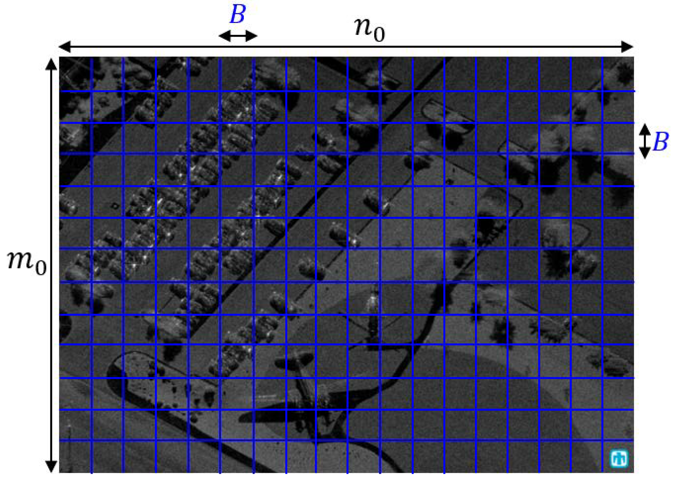
Let us define a square block with pixels. For convenience, suppose that and are integer multiples of B, respectively, in an image, and define r as the measurement ratio (). When the image size is large (i.e., and ), the conventional CS-based compression and reconstruction of images require excessive computational complexity because the dimensions of the measurement matrix are given by . To reduce the computational load, the whole image is divided into multiple blocks with pixels as shown in Figure 1. Then, the total number of blocks is and the compressed image is denoted as
where is the original signal vector obtained by stacking the original 2D image into a vector, is the measurement matrix commonly used for each block, is the number of measured samples per block, is the compressed signal vector, and is the measurement noise vector with zero mean. For example, when is a random sampling matrix that randomly selects M elements from pixels, is composed of M rows randomly selected from . Since the same measurement matrix is applied to all blocks for CS, the signal model in (4) can be represented as
where , , and are formed by reshaping , , and , respectively.
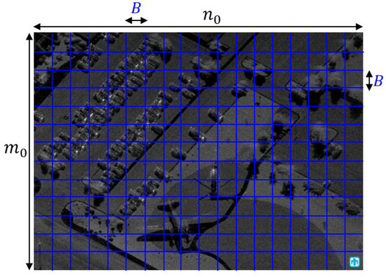
Figure 1.
Image partitioning into multiple blocks (original SAR image from [51]).
2.3. Reconstruction by BCS-SPL with Fixed Measurement Ratio
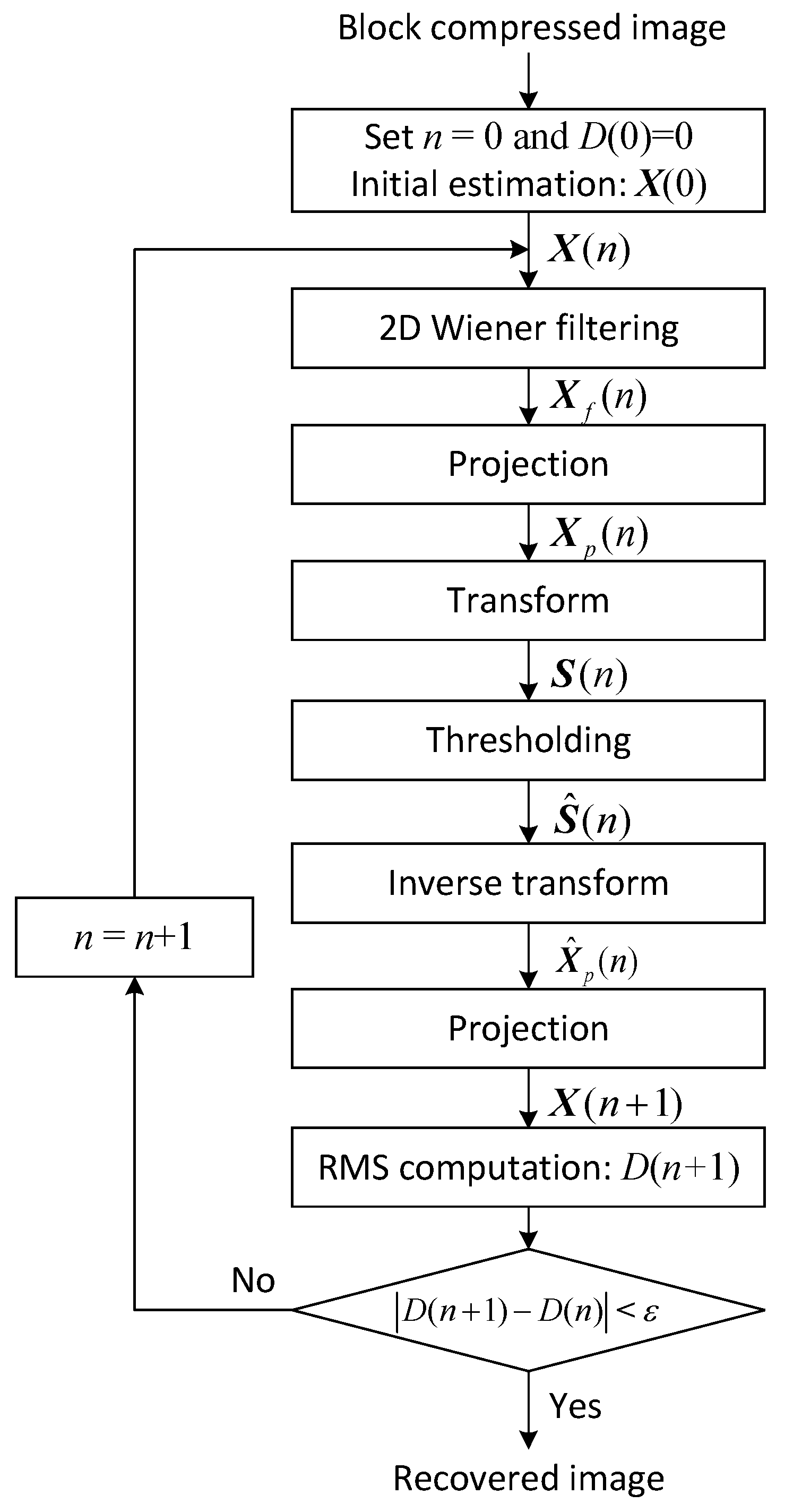
Figure 2 describes the smoothed projected Landweber (SPL) algorithm combined with BCS that iteratively reconstructs the original image from the block compressed image with fixed measurement ratio by repeating 2D Wiener filtering, convex projection, and thresholding in the transform domain. Initially, when is known, the matrix in (5) can be estimated in the least squares (LS) sense from the compressed image as follows:
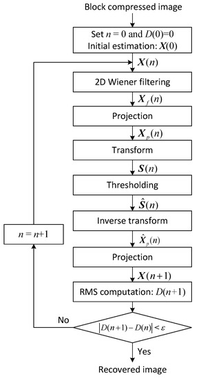
Figure 2.
Image reconstruction using BCS-SPL [14,15].
In the n-th iteration, is converted to the image and 2D Wiener filtering is carried out to alleviate the artifacts caused by blockwise image reconstruction. The filtered image is recovered to the signal matrix and then the i-th column of is projected to the hyper-plane to find the closest vector on where is the i-th column of and . Because the same measurement matrix is applied to all blocks, the projected matrix is denoted as
Here, the second term of (7) is the projection of the error matrix between and to meet the constraint . For sparse representation, is again converted to through some transform , i.e.,
For example, the DCT, DWT, and DDWT can be used for . To increase the sparsity of the transform-domain coefficients, the bivariate shrinkage in [19] is used for thresholding as follows:
where is a convergence-control factor with a positive real value and the operator is given by
Here, means the parent coefficients of x in the next coarser scale, is the marginal standard deviation of x estimated in a local neighborhood around x, , and . By the inverse transform of , we have
and again by projecting onto the hyper-plane, we obtain
Finally, the mean square error (MSE) between and is computed as
and the loop is repeated until where is the tolerance parameter.
2.4. Fully Adaptive BCS and Blockwise Image Reconstruction
In this subsection, we introduce an adaptive BCS method in which an individual block has a different measurement ratio in the range of determined by several criteria such as the variance, the equivalent noise level, and the local salient factor in each block [20,21,34]. For example, when the measurement ratio is determined according to the variance of each image block, the number of measurements for the ith block is computed as
where is the variance of the ith block and . In this case, each block employs a dedicated measurement and thus the image compression procedure is denoted as
where , , , and are the compressed signal vector, the measurement matrix, the vector of the original image, and the noise vector in the ith block, respectively. Moreover, the BCS image reconstruction described in Figure 2 is separately carried out for each block using and thus, (7) and (12) are changed as follows:
where . As shown in Figure 2, the BCS-SPL algorithm requires iterative computation of and from the error vectors and . Whereas this projection process is performed in the matrix form as in (7) and (12) for the BCS-SPL with a fixed measurement ratio, the projected vector is separately evaluated using a different as in (16) and () for the BCS-SPL with fully adaptive measurement ratios. Therefore, the adaptive BCS methods in [20,21,34] increase the compression efficiency by allowing an arbitrary measurement ratio over , however the amount of side information is very large and the computational load for image reconstruction is very high due to the increased number of measurement matrices. Note that the cardinality of is in the worst case.
3. Proposed Clustered BCS with Quantized Measurement Ratio
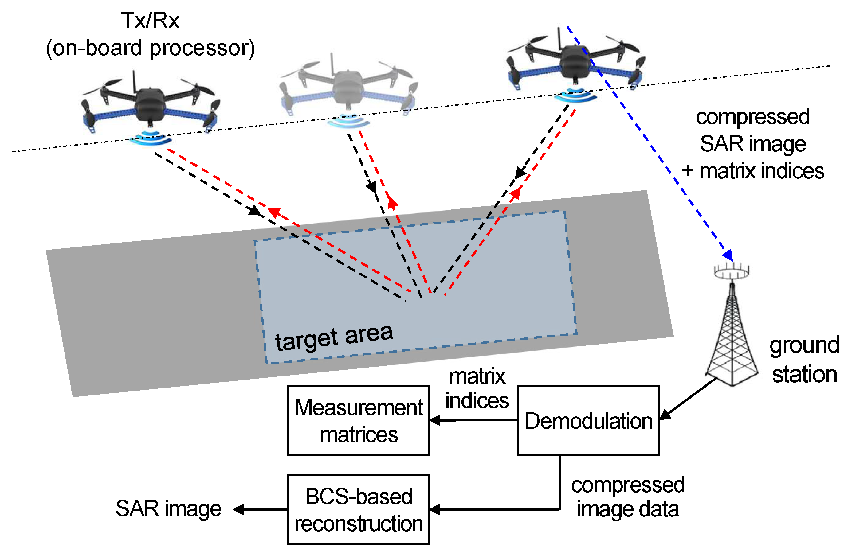
In this section, we consider a SAR imaging system that performs image compression in the on-board processor of a remote sensing node and image reconstruction in the ground station, as shown in Figure 3. For image reconstruction, the remote sensing node transfers the compressed data along with the information about measurement matrices. In an attempt to reduce the overhead to transfer measurement matrix indices and the computational complexity for reconstructing SAR images, we propose a new clustered BCS scheme with quantized measurement ratio. The measurement ratio for each block is selected from the predetermined quantized values depending on the blockwise sparsity of wavelet coefficients. The original image is reconstructed by using the clustered BCS-SPL method that classifies the blocks into clusters according to the measurement ratio and concurrently performs the BCS-SPL algorithm for clustered blocks.
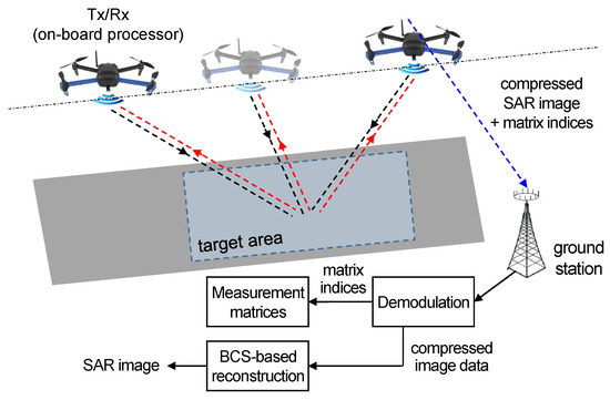
Figure 3.
Drone SAR image processing using the proposed clustered BCS.
3.1. Selection of Measurement Ratio
In a SAR image, the blocks including a specific target have more information than the blocks corresponding to the background region. To estimate the amount of information for an individual block, the 2D DDWT is carried out to obtain the subband coefficients representing six wavelet orientations. Suppose that is a matrix obtained by reshaping the magnitude of the complex SAR image . By performing the DDWT for , we have
where means the DDWT operation, is the level 1 DDWT coefficients for the sth subband, and . Here, for notational convenience, we neglected 2D matrix extension near image edges to mitigate coefficient distortion. To sparsely represent the DDWT coefficients, the thresholding function in (10) is employed as below:
where the level 2 DDWT coefficients are used for the parent coefficients . Now, considering the size reduction in the DDWT, is divided into blocks with pixels, and then the number of nonzero elements is counted to compute the amount of information in each block.
Let us denote the number of nonzero elements in the ith block of as . Then, the total number of nonzero elements in the ith block is computed as
where . Define K as the number of measurement matrices. Using in (20), the measurement ratio for the ith block is selected from K quantized values as follows:
- Compute the ratio of nonzero elements:
- Quantize with parameter :
- Remove the bias in :
- Compute the block measurement ratio by scaling :where and are given by
Here, is a parameter to determine the quantization stepsize; is a positive parameter to ensure for all i, i.e., defines the minimum block measurement ratio; and and are scaling factors to satisfy that the average of is equal to r, i.e., . The parameters and are pre-determined by a numerical grid search using SAR images for training, and a practical design example is presented in Section 5.1.
3.2. SAR Image Compression Using Quantized Measurement Ratio
From the procedure in (21)–(25), the measurement ratio for each block is determined by one of K quantized values depending on the sparsity of DDWT coefficients. Denote the set including K quantized measurement ratios as , and then for all i, i.e., is selected from the codebook . For SAR image compression, we generate random measurement matrices corresponding to by using the design method in [52]. Specifically, structurally random matrices are expressed as
where
- is a subsampling matrix where . can be generated by randomly selecting rows of . This matrix selects a random subset of rows of .
- is an orthogonal transform matrix. In the proposed method, is defined as the inverse DCT matrix. This matrix is used to spread the SAR image information over all measurements.
- is a random permutation matrix for scrambling the signal locations. This matrix is also called the global randomizer.
Here, has orthonormal row vectors, i.e., . Note that the candidates of and are pre-determined and shared in the remote sensing node and the ground station as codebooks, respectively.
The original SAR image is partitioned into blocks with pixels, and then the blocks are classified into K clusters according to the measurement ratio. Define the number of blocks in the kth cluster as . The blocks in the kth cluster can be compressed using the same measurement matrix as follows:
where is the compressed sub-image matrix for kth cluster, is the original sub-image matrix for kth cluster, is the original image signal vector for the cth block whose measurement ratio is equal to , is the compressed signal vector corresponding to , and is the noise matrix for kth cluster. Because the same measurement matrix is applied to the blocks in a cluster as shown in (27), the compression procedure can be effectively implemented through parallel processing and pipeline architectures [53]. The SAR image compression in (27) is repeated for all clusters, and thus the computational complexity is proportional to the number of clusters K.
3.3. SAR Image Reconstruction Using Clustered BCS Algorithm
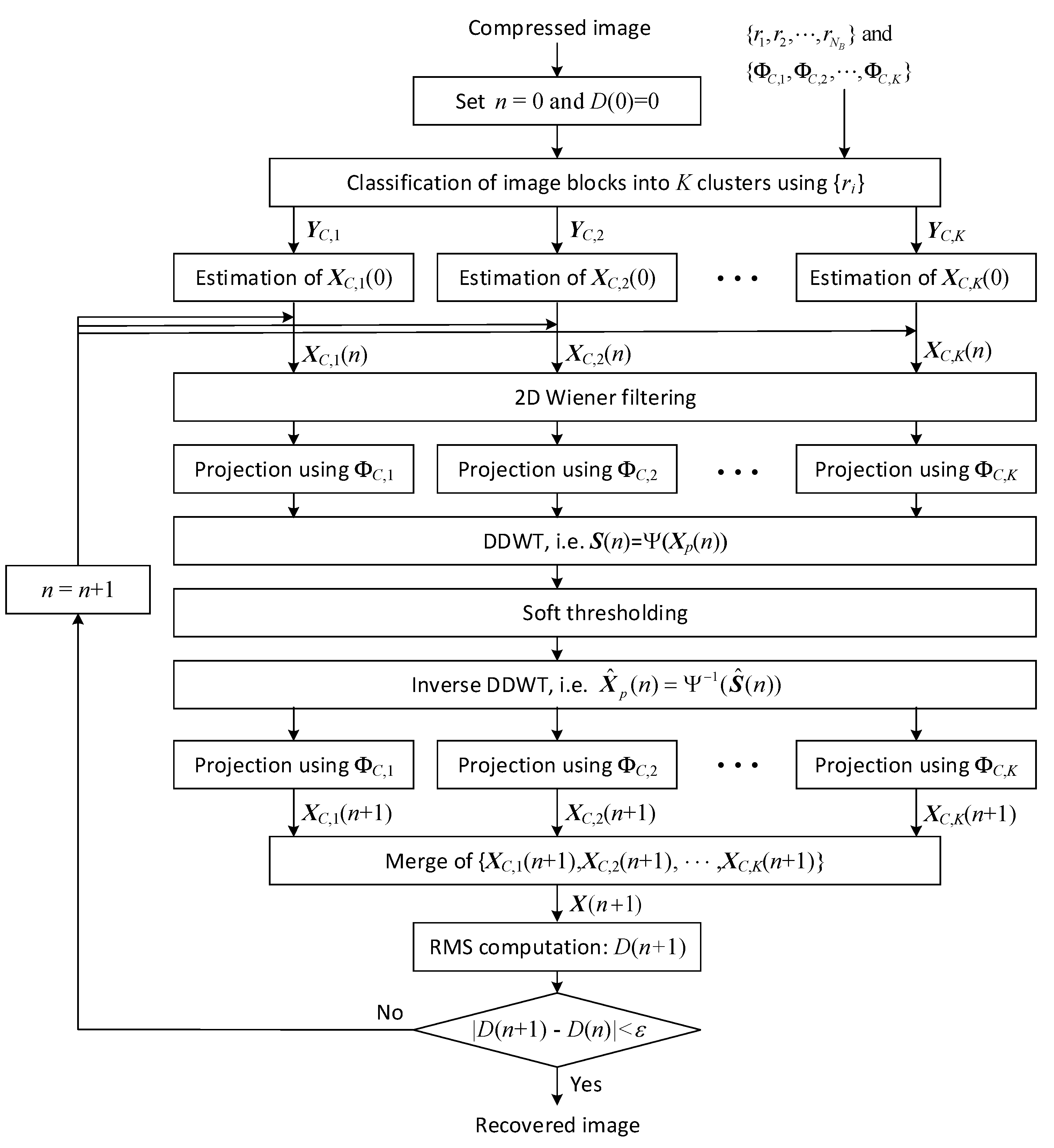
In this subsection, we propose an adaptive BCS algorithm that reconstructs the SAR image using the clustered structure of a compressed image. Figure 4 describes the overall procedure of the proposed adaptively clustered BCS algorithm when the BCS-SPL is employed for sub-image reconstruction in each cluster. As shown in Figure 3, the received data from the remote sensing node are divided to the compressed image and the information about and , respectively. After the initialization step, the compressed image blocks are classified into K clusters according to the block measurement ratio. Because the blocks in a cluster have the same measurement ratio, the measurement matrix can be commonly used to reconstruct the sub-image corresponding to the cluster, and thus the computational load is reduced by virtue of parallel processing and pipeline architectures.

Figure 4.
Image reconstruction using the proposed clustered BCS.
In the kth cluster, the initial sub-image matrix is estimated in the LS sense using the compressed matrix as follows:
where . Then, the BCS-SPL algorithm is separately performed for each cluster as shown in Figure 4. In the n-th iteration, is obtained by aggregating and 2D Wiener filtering is carried out to mitigate the artifacts.
The filtered image is converted to the signal matrix for the kth cluster, , and then is separately projected onto the hyper-plane as follows:
where is the projected matrix for kth cluster and . are merged to , and is converted to through the DDWT for sparse representation, i.e.
As in (9) and (10), the soft thresholding is applied to to increase the sparsity of the transform-domain coefficients. By taking the inverse DDWT to the thresholding operator output , we have
is divided into the sub-images corresponding to K clusters. When denoting the inverse transformed sub-image for the kth cluster as , the sub-image is projected onto the hyper-plane again as below:
4. Measurement for SAR Imaging
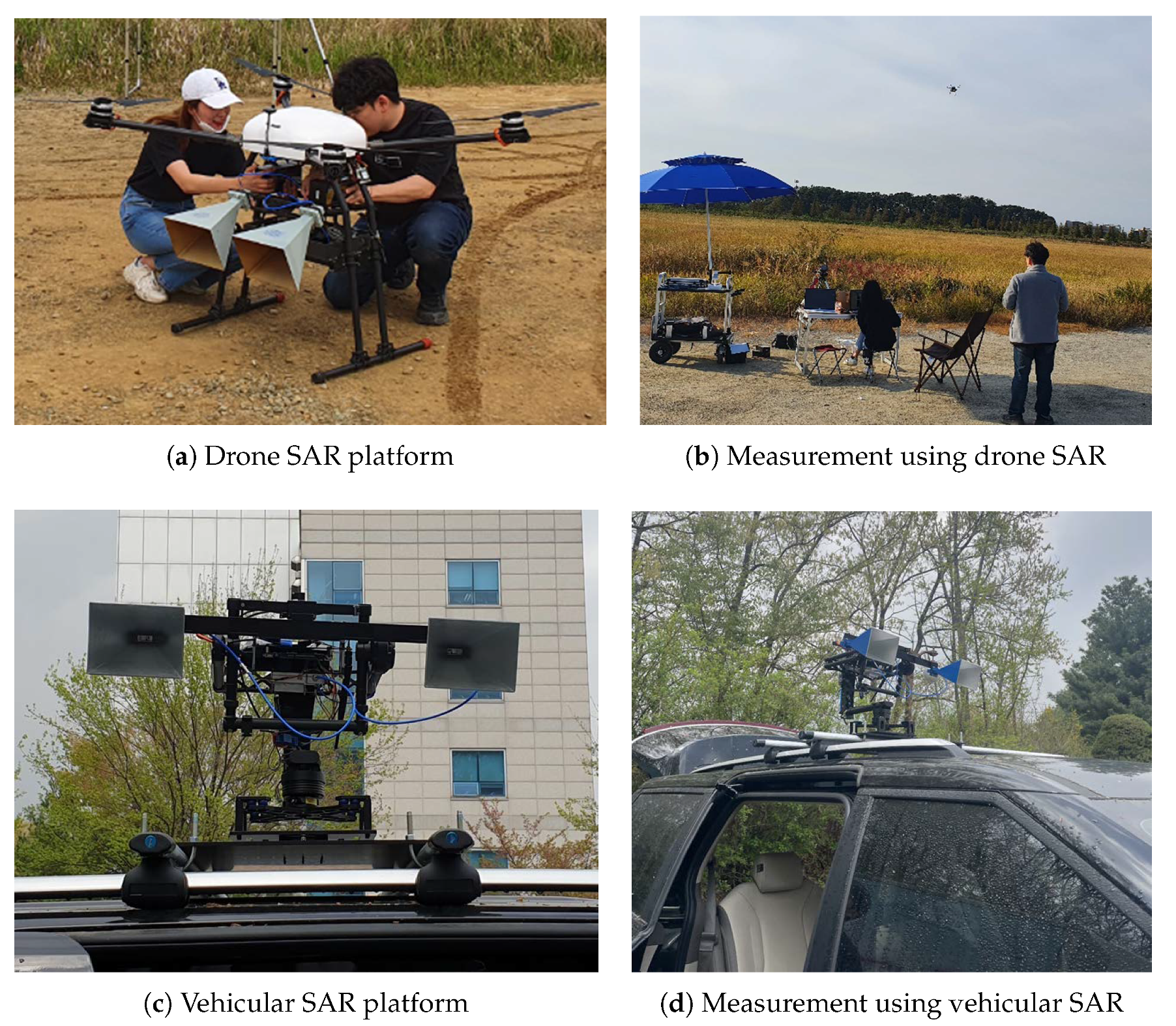
To obtain real SAR images, we performed field tests using self-made drone SAR and vehicular SAR systems. Figure 5 shows two SAR platforms composed of a transceiver for frequency modulated continuous wave (FMCW) radar and two horn antennas, respectively. These SAR platforms are mounted on the underside of the drone and on the roof of the test vehicle for field measurement. The field tests were carried out in Daebu Island of South Korea and near the tennis court of Korea Aerospace University for the drone SAR and the vehicular SAR, respectively, and the parameters in Table 1 were used for sensing echo signals. The recording time per test is in the range of 60∼90 s, and a filtering technique was exploited to mitigate the interference caused by clutters. The RDA described in Section 2.1 was used to generate real SAR images from the measured sensing data in both SAR systems. The real SAR images obtained by field measurement data are presented in the next section.
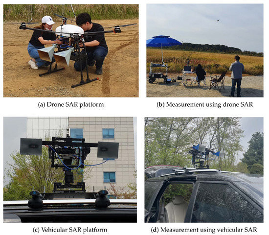
Figure 5.
Self-made SAR systems and field measurement.

Table 1.
Parameters for drone SAR and vehicular SAR systems.
5. Simulation Results
This section evaluates the performance of the proposed BCS method with quantized adaptive measurement ratio in terms of the peak signal-to-noise ratio (PSNR) of reconstructed images, by applying the proposed technique to the real SAR images in [51] and experimental data obtained by self-made drone SAR and vehicular SAR systems in Section 4. Moreover, through numerical simulations, the proposed method is compared to the existing BCS-based image compression methods in terms of the PSNR and the execution time. In the following simulations, we use the SAR test images in Table 2, and set the block size to for BCS.
Table 2.
SAR images for performance evaluation (the images 1∼4 are available by courtesy of Sandia National Lab., Radar ISR [51] and the images 5 and 6 are obtained by field measurement in Section 4).
5.1. Parameter Optimization for Proposed Clustered BCS
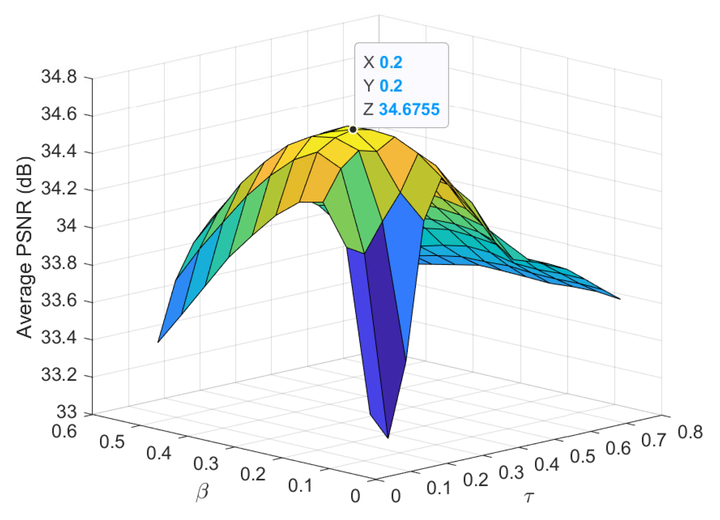
In the proposed clustered BCS, the measurement ratio selection procedure in (21)–(25) requires the design of the parameters and . The parameter adjusts the stepsize for quantization of initial block measurement ratios , while determines the relative ratio of the minimum block measurement ratio to the average value, i.e., . We find the optimal values of and through 2D grid search in the range of and . In the simulation, we used and , and the stepsize for 2D grid search was set to considering accuracy and runtime. Figure 6 presents the average PSNR of SAR images reconstructed by the proposed clustered BCS according to and , when the test images 1,3, and 4 in Table 2 were used. Note that the image 2 was not used because its high resolution requires excessive execution time for grid search. It is shown that the proposed method achieves the highest average PSNR when and . Also, notice that the average PSNR is quite robust around the optimal and , for example, in the range of and .
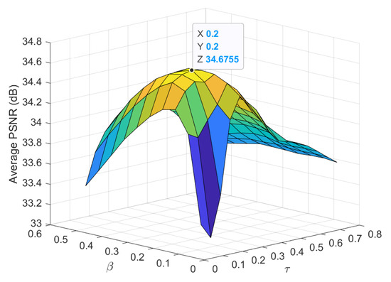
Figure 6.
PSNR of the proposed clustered BCS according to and when and .
The proposed scheme necessitates the design of the number of measurement matrices K (or the number of clusters for reconstruction). To this end, the performance of the proposed clustered BCS method is evaluated for various K and r in terms of PSNR in Figure 7, when and . The proposed methods with achieve huge PSNR gains compared to the fixed-ratio BCS in [15] corresponding to . As expected, the PSNR performance of the proposed scheme gradually improves with the increment of K irrespective of the average measurement ratio r. When , , and , the maximum PSNR loss is less than 0.12 dB, 0.05 dB, and 0.01 dB, respectively, compared to the case with . Through the tradeoff between the PSNR loss and the computational complexity, we set in the following simulations.
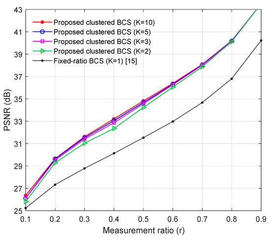
Figure 7.
PSNR of the proposed clustered BCS for the various number of measurement matrices K when and .
5.2. Reconstructed Image Performance and Runtime
The proposed clustered BCS method is compared to the existing BCS-based compression schemes for SAR images. Specifically, the following reconstruction techniques are considered.
- Fixed-ratio BCS: the method in [15] is used. All blocks are compressed with the same measurement ratio, and SAR images are reconstructed by the BCS-SPL in Section 2.3.
- Fully adaptive BCS: the method in [34] is used. Block measurement ratios are assigned according to block variances in the image-domain, and SAR images are reconstructed by separately applying the BCS-SPL to each block as explained in Section 2.4. The minimum block measurement ratio is set to 0.001 to avoid the numerical instability in the BCS-SPL algorithm.
- Proposed clustered BCS: The block measurement ratio is adaptively assigned with quantization using the procedure in Section 3.1, the original image is compressed as explained in Section 3.2, and the SAR image is reconstructed by the proposed clustered BCS in Section 3.3. The parameters are set as , , and , and the random sampling matrices are defined as (26), unless otherwise specified.
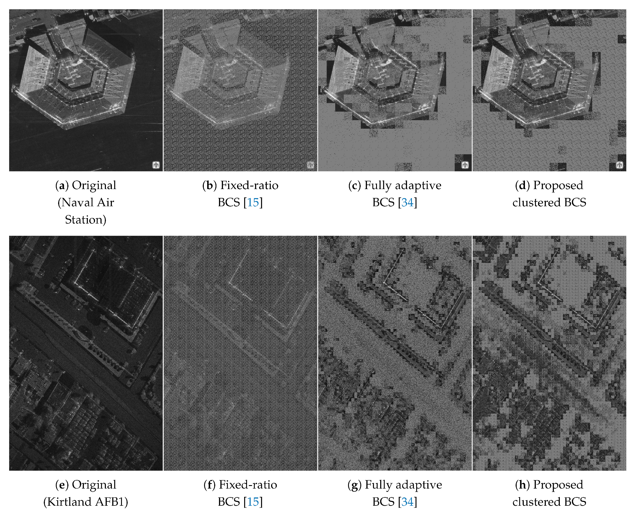
Figure 8 compares the original SAR image with the compressed images using the fixed-ratio BCS, fully adaptive BCS, and proposed clustered BCS methods, respectively. We used random sampling matrices, i.e., , to visualize the difference among BCS-based compression schemes. The fixed-ratio BCS subsamples blocks with the same measurement ratio, and thus the sub-image resolution is identical to all blocks. In contrast, the sub-image resolution significantly varies according to the block sparsity in the fully adaptive BCS and the proposed clustered BCS. Especially, the fully adaptive BCS scheme exhibits more variation of sub-image resolution due to the high deviation of block measurement ratios. Notice that the block size of Kirtland AFB1 looks smaller than that of Naval Air Station, because Kirtland AFB1 has more pixels than Naval Air Station as shown in Table 2.
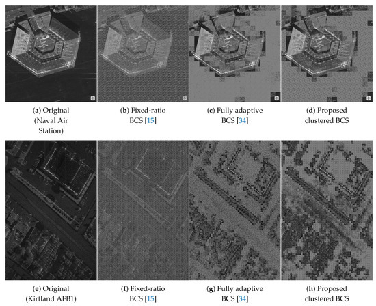
Figure 8.
Reconstructed SAR images using various BCS methods when .
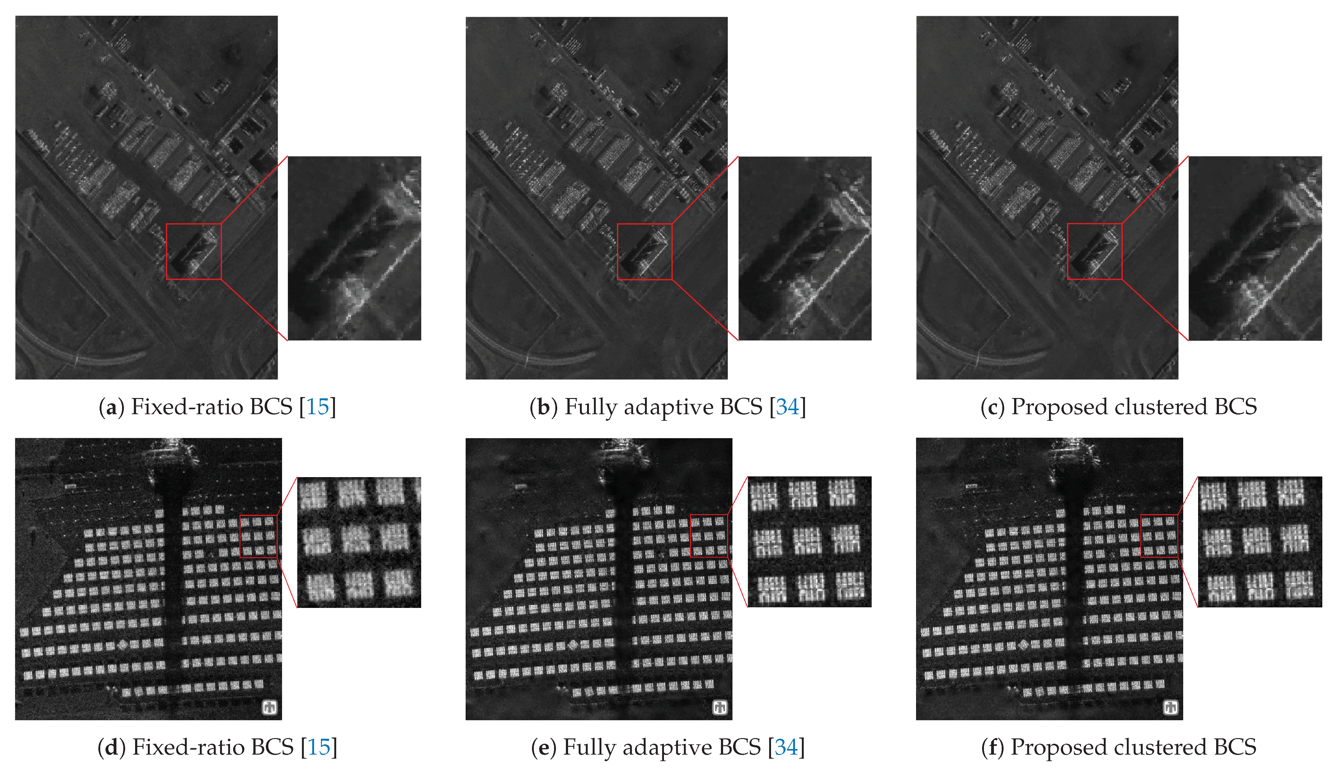
Figure 9 compares the reconstructed images by the various BCS-based methods. The test images 3 (Kirtland AFB2) and 4 (Solar Tower) are used for the original SAR images, and the measurement ratio is set to 0.5, i.e., . We enlarged a specific area of the SAR image to clearly compare the restored image quality. For example, a building is magnified in Kirtland AFB2, and a solar panel is enlarged in Solar Tower. The fully adaptive BCS and proposed methods obtain SAR images with higher quality than the fixed-ratio BCS, as seen in the target objects indicated as red boxes. Because the proposed clustered BCS has higher minimum block measurement ratio than the fully adaptive BCS, the image quality of the proposed BCS is slightly better than the fully adaptive BCS around the background region.
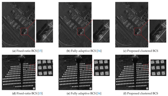
Figure 9.
Reconstructed SAR images using various BCS methods when . The original images are Kirtland AFB2 for (a)∼(c) and Solar Tower for (d)∼(f).
Figure 10a,d show the optical images of the locations where the field tests were carried out to obtain real SAR images. When the proposed clustered BCS method is applied to the measured drone SAR and vehicular SAR images, we can successfully reconstruct the SAR images similar to the optical counterparts. Even when , i.e., just 10% of measured SAR image data are used, main objects such as warehouses and fences can be recognized in the restored images. As expected, the quality of reconstructed images is significantly improved when , compared to the case when . For the vehicular SAR, the field measurement was conducted while driving along the road in the lower part of Figure 10d. Therefore, the SAR images clearly present the fences near the lower road, yet the image quality is degraded as the distance from the lower road increases.
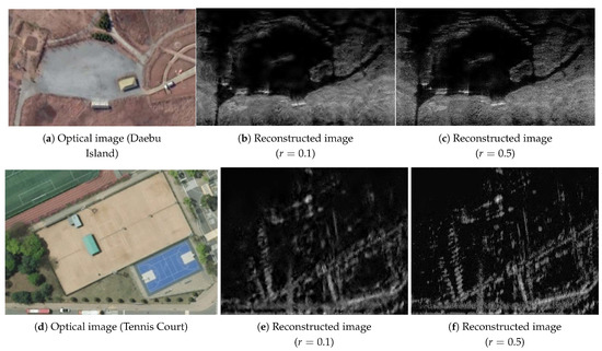
Figure 10.
SAR images reconstructed by the proposed clustered BCS method. (a,d) denote the optical satellite images of test locations in Daebu Island and Tennis Court in Korea Aerospace University, respectively.
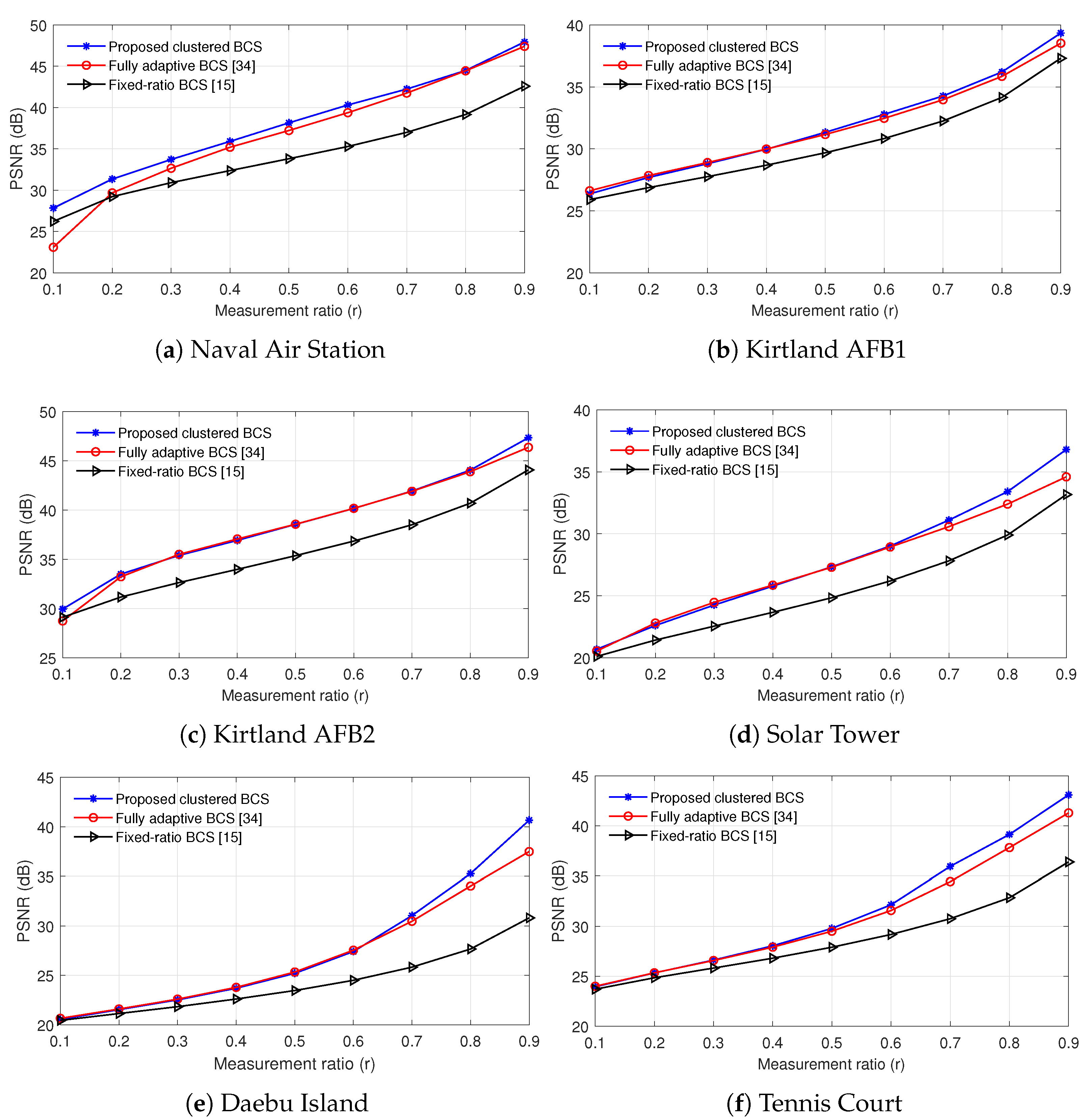
Figure 11 compares the PSNR performance of various BCS reconstruction algorithms when the test images in Table 2 are used. For the proposed method, we used , , and . Every PSNR value was obtained by averaging the results over more than 20 random realizations of measurement matrices. The proposed clustered BCS outperforms the fixed-ratio BCS in all test images, and the PSNR gain gradually becomes large as the measurement ratio increases. The proposed scheme performs comparable or better than the fully adaptive BCS method in all test images, while the PSNR gap is very small in the range of except Naval Air Station and slightly increases with the increment of the measurement ratio when . In the fully adaptive BCS, the deviation of r is large as inferred from (14). Thus, when , most blocks have measurement ratios close to one and a part of blocks have very low ratios, resulting to PSNR degradation. Overall, the proposed method exhibits the best PSNR performance in all test images irrespective of r.
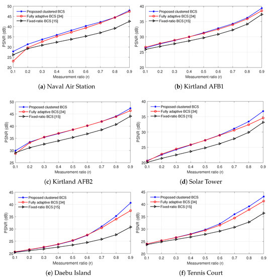
Figure 11.
PSNR of various BCS reconstruction methods according to the measurement ratio.
Table 3 shows the specific mean and standard deviation values of PSNR corresponding to Figure 11. As mentioned before, PSNR values were obtained by repeating the simulations for more than 20 random realizations of measurement matrices. When , the average PSNR gain of the proposed clustered BCS is in the range of dB compared to the fixed-ratio BCS and dB compared to the fully adaptive BCS. When , the average PSNR gain of the proposed method is changed to dB compared to the fixed-ratio BCS and over the fully adaptive BCS. When , the average PSNR gain is in the range of dB and dB compared to the fixed-ratio BCS and the fully adaptive BCS, respectively. Overall, as r becomes large, the PSNR gain grows accordingly. The standard deviation of the proposed method is slightly greater than that of the fixed-ratio BCS and very similar to the fully adaptive BCS. For all cases, the standard deviation of PSNR is less than 0.1 dB, and thus the PSNR variation by the measurement matrices is almost negligible.
Table 3.
Mean () and standard deviation () of PSNR for various BCS reconstruction methods.
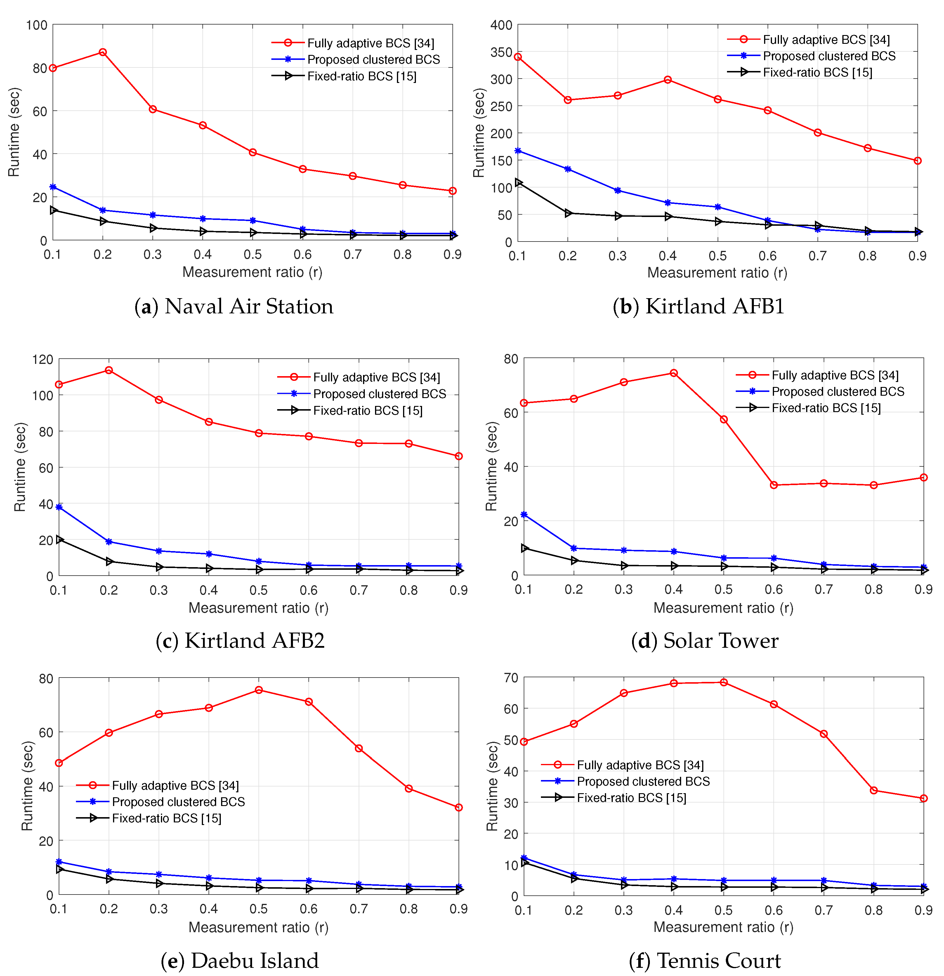
To compare the complexity of various BCS reconstruction methods, Figure 12 presents the runtime when the SAR test images in Table 2 are used. The BCS reconstruction methods were programmed by MATLAB v9.9.0, and the execution time was measured using a desktop PC with Core i7-10700KF 3.8 GHz CPU, 16 GB RAM, and 64-bit Windows 10. Because the execution time for SAR image compression is less than 5% of the runtime for reconstruction in all BCS schemes, we only consider the execution time for SAR image reconstruction. As mentioned before, the parameters and are fixed when recording the runtime, i.e., and , and thus the execution time for designing and is not taken into account. Every runtime value was obtained by averaging the results over more than 20 random realizations of measurement matrices. As expected in reconstruction algorithms in Section 2.3, Section 2.4, and Section 3.3, the fixed-ratio BCS has the lowest runtime, the fully adaptive BCS exhibits the highest runtime, and the proposed method requires slightly more execution time than the fixed-ratio BCS in all test images. On average, the runtime of the proposed scheme is 1.27∼2.56 times greater than that of the fixed-ratio BCS, whereas the runtime of the fully adaptive BCS is 5.04∼20.15 times greater than that of the fixed-ratio BCS. The fully adaptive BCS and proposed BCS methods tend to require less execution time as r increases, due to the decrease of the number of iterations for the BCS-SPL algorithm. Figure 11 and Figure 12 show that the proposed clustered BCS is advantageous over the fixed-ratio BCS and fully adaptive BCS techniques, when jointly taking into account the PSNR performance and the runtime.
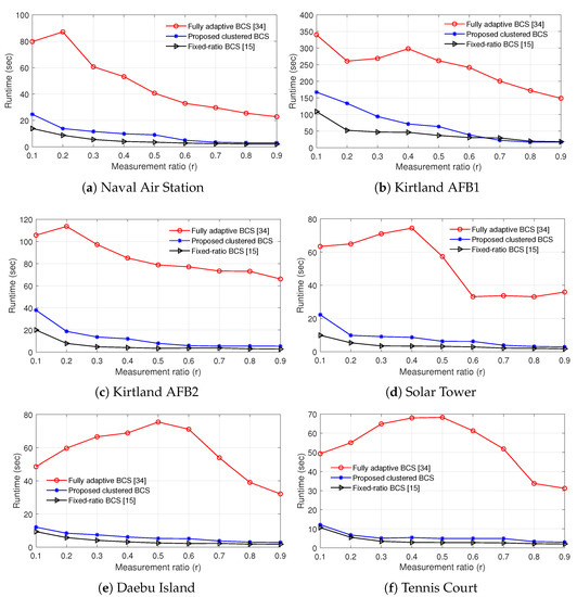
Figure 12.
Runtime of various BCS reconstruction methods according to the measurement ratio.
6. Conclusions
In this paper, we proposed a new quantization method of block measurement ratios for SAR image compression based on the clustered BCS, and derived the reconstruction algorithm that classifies the blocks into clusters according to the measurement ratio and iteratively recovers the SAR sub-image cluster-wise. The proposed BCS method increases the overall compression efficiency by assigning a higher measurement ratio to the block with more nonzero coefficients and a lower ratio to that with fewer nonzero coefficients. In addition, the codebook size for measurement matrices can be reduced through quantization of block measurement ratios, thereby alleviating the increase in computational complexity. For intensive performance verification, the proposed scheme has been applied to multiple SAR images obtained from airborne, drone and vehicular SAR platforms, respectively. The image properties from different platform types exhibit significant variations with regards to speckle noises and contrast levels but the proposed scheme maintains consistent performances for all cases. For this reason, the PSNR performance of the reconstructed SAR image is significantly improved at the cost of a moderate complexity increase compared to the conventional fixed-ratio BCS. foopinkfooWith much reduced computational load, the proposed scheme achieves PSNR performances that are comparable to the fully adaptive BCS.
Recent deployment of video SAR demands a huge amount of data samples with the increased frame rates in high resolutions. While this poses significant challenges for data collection and storage, our work can be employed to relieve the burden of dealing with these problems. The proposed technique can be applied to the compression of drone SAR images and further extended to compressing video SAR of higher frames in order to alleviate the storage limitation while minimizing the image quality loss. Through this approach, the drone SAR can be utilized in more diverse applications such as detection of landmines, military surveillance, and lifesaving in case of disasters. In future, further research works are expected for clustered SAR missions by adopting the proposed clustered BCS for SAR raw data compression.
Author Contributions
J.C. designed the conceptual algorithm and performed computer simulations; W.L. is in charge of the field measurement for obtaining SAR raw data and provided guidance for this research; J.C. and W.L. wrote and revised the paper. All authors have read and agreed to the published version of the manuscript.
Funding
The authors gratefully acknowledge the support from Next Generation SAR Laboratory at Korea Aerospace University, originally funded by Defense Acquisition Program Administration (DAPA) and Agency for Defense Development (ADD).
Institutional Review Board Statement
Not applicable.
Informed Consent Statement
Not applicable.
Data Availability Statement
Not applicable.
Acknowledgments
The authors thank the Sandia National Laboratories, Radar ISR for providing real SAR images through the website.
Conflicts of Interest
The authors declare no conflict of interest.
References
- Donoho, D.L. Compressed sensing. IEEE Trans. Inf. Theory 2006, 52, 1289–1306. [Google Scholar] [CrossRef]
- Candes, E.J.; Romberg, J.; Tao, T. Robust uncertainty principles: Exact signal reconstruction from highly incomplete frequency information. IEEE Trans. Inf. Theory 2006, 52, 489–509. [Google Scholar] [CrossRef] [Green Version]
- Candes, E.J.; Tao, T. Near-Optimal Signal Recovery From Random Projections: Universal Encoding Strategies? IEEE Trans. Inf. Theory 2006, 52, 5406–5425. [Google Scholar] [CrossRef] [Green Version]
- Haupt, J.; Nowak, R. Signal Reconstruction From Noisy Random Projections. IEEE Trans. Inf. Theory 2006, 52, 4036–4048. [Google Scholar] [CrossRef]
- Gill, P.R.; Wang, A.; Molnar, A. The In-Crowd Algorithm for Fast Basis Pursuit Denoising. IEEE Trans. Signal Process. 2011, 59, 4595–4605. [Google Scholar] [CrossRef]
- Quan, X.; Zhao, X.; Yang, J.; Xie, X.; Bao, W.; Zhang, B.; Wu, Y. 3-D Scattering Center Extraction Based on BPDN for Complex Radar Targets. In Proceedings of the 2019 IEEE International Geoscience and Remote Sensing Symposium (IGARSS), Yokohama, Japan, 28 July–2 August 2019; pp. 3756–3759. [Google Scholar] [CrossRef]
- Cai, T.T.; Wang, L. Orthogonal Matching Pursuit for Sparse Signal Recovery With Noise. IEEE Trans. Inf. Theory 2011, 57, 4680–4688. [Google Scholar] [CrossRef]
- Needell, D.; Vershynin, R. Signal Recovery From Incomplete and Inaccurate Measurements Via Regularized Orthogonal Matching Pursuit. IEEE J. Sel. Top. Signal Process. 2010, 4, 310–316. [Google Scholar] [CrossRef] [Green Version]
- Needell, D.; Tropp, J. CoSaMP: Iterative signal recovery from incomplete and inaccurate samples. Appl. Comput. Harmon. Anal. 2008, 26, 301–321. [Google Scholar] [CrossRef] [Green Version]
- Donoho, D.L.; Tsaig, Y.; Drori, I.; Starck, J. Sparse Solution of Underdetermined Systems of Linear Equations by Stagewise Orthogonal Matching Pursuit. IEEE Trans. Inf. Theory 2012, 58, 1094–1121. [Google Scholar] [CrossRef]
- Wang, J.; Kwon, S.; Li, P.; Shim, B. Recovery of Sparse Signals via Generalized Orthogonal Matching Pursuit: A New Analysis. IEEE Trans. Signal Process. 2016, 64, 1076–1089. [Google Scholar] [CrossRef] [Green Version]
- Donoho, D.L.; Maleki, A.; Montanari, A. Message passing algorithms for compressed sensing: I. motivation and construction. In Proceedings of the 2010 IEEE Information Theory Workshop on Information Theory (ITW), Cairo, Egypt, 6–8 January 2010; pp. 1–5. [Google Scholar] [CrossRef] [Green Version]
- Donoho, D.L.; Maleki, A.; Montanari, A. Message passing algorithms for compressed sensing: II. analysis and validation. In Proceedings of the 2010 IEEE Information Theory Workshop on Information Theory (ITW), Cairo, Egypt, 6–8 January 2010; pp. 1–5. [Google Scholar] [CrossRef] [Green Version]
- Gan, L. Block Compressed Sensing of Natural Images. In Proceedings of the 15th International Conference on Digital Signal Processing (ICDSP), Cardiff, UK, 1–4 July 2007; pp. 403–406. [Google Scholar] [CrossRef]
- Mun, S.; Fowler, J.E. Block Compressed Sensing of Images Using Directional Transforms. In Proceedings of the 16th IEEE International Conference on Image Processing (ICIP), Cairo, Egypt, 7–10 November 2010; p. 547. [Google Scholar] [CrossRef]
- Fowler, J.E.; Mun, S.; Tramel, E.W. Multiscale block compressed sensing with smoothed projected Landweber reconstruction. In Proceedings of the 19th European Signal Processing Conference (EUSIPCO), Barcelona, Spain, 29 August–2 September 2011; pp. 564–568. [Google Scholar]
- Unde, A.S.; Deepthi, P. Block compressive sensing: Individual and joint reconstruction of correlated images. J. Vis. Commun. Image R. 2017, 44, 187–197. [Google Scholar] [CrossRef]
- Shi, C.; Wang, L.; Zhang, J.; Miao, F.; He, P. Remote Sensing Image Compression Based on Direction Lifting-Based Block Transform with Content-Driven Quadtree Coding Adaptively. Remote Sens. 2018, 10, 999. [Google Scholar] [CrossRef] [Green Version]
- Sendur, L.; Selesnick, I.W. Bivariate shrinkage functions for wavelet-based denoising exploiting interscale dependency. IEEE Trans. Signal Process. 2002, 50, 2744–2756. [Google Scholar] [CrossRef] [Green Version]
- Hubbard-Featherstone, C.J.; Garcia, M.A.; Lee, W.Y.L. Adaptive block compressive sensing for image compression. In Proceedings of the 2017 International Conference on Image and Vision Computing New Zealand (IVCNZ), Christchurch, New Zealand, 4–6 December 2017; pp. 1–6. [Google Scholar] [CrossRef]
- Zhu, Y.; Liu, W.; Shen, Q. Adaptive Algorithm on Block-Compressive Sensing and Noisy Data Estimation. Electronics 2019, 8, 753. [Google Scholar] [CrossRef] [Green Version]
- Rilling, G.; Davies, M.; Mulgrew, B. Compressed sensing based compression of SAR raw data. In Proceedings of the SPARS’09—Signal Processing with Adaptive Sparse Structured Representations, Saint-Malo, France, 6–9 April 2009; pp. 1–6. [Google Scholar]
- Boufounos, P.T. Universal Quantization and SAR Compression; Technical Report; Mitsubishi Electric Research Laboratories, Inc.: Cambridge, MA, USA, 2019. [Google Scholar]
- Yang, H.; Chen, C.; Chen, S.; Xi, F. Sub-Nyquist SAR via Quadrature Compressive Sampling with Independent Measurements. Remote Sens. 2019, 11, 472. [Google Scholar] [CrossRef] [Green Version]
- Samadi, S.; Çetin, M.; Masnadi-Shirazi, M.A. Sparse Representation-Based Synthetic Aperture Radar Imaging. IET Radar Sonar Navig. 2011, 5, 182–193. [Google Scholar] [CrossRef] [Green Version]
- Fang, J.; Xu, Z.; Zhang, B.; Hong, W.; Wu, Y. Fast Compressed Sensing SAR Imaging Based on Approximated Observation. IEEE J. Sel. Top. Appl. Earth Obs. Remote Sens. 2014, 7, 352–363. [Google Scholar] [CrossRef] [Green Version]
- Ao, D.; Wang, R.; Hu, C.; Li, Y. A Sparse SAR Imaging Method Based on Multiple Measurement Vectors Model. Remote Sens. 2017, 9, 297. [Google Scholar] [CrossRef] [Green Version]
- Liang, L.; Li, X.; Ferro-Famil, L.; Guo, H.; Zhang, L.; Wu, W. Urban Area Tomography Using a Sparse Representation Based Two-Dimensional Spectral Analysis Technique. Remote Sens. 2018, 10, 109. [Google Scholar] [CrossRef] [Green Version]
- Luo, H.; Li, Z.; Dong, Z.; Yu, A.; Zhang, Y.; Zhu, X. Super-Resolved Multiple Scatterers Detection in SAR Tomography Based on Compressive Sensing Generalized Likelihood Ratio Test (CS-GLRT). Remote Sens. 2019, 11, 1930. [Google Scholar] [CrossRef] [Green Version]
- Wu, C.; Zhang, Z.; Chen, L.; Yu, W. Super-Resolution for MIMO Array SAR 3-D Imaging Based on Compressive Sensing and Deep Neural Network. IEEE J. Sel. Top. Appl. Earth Obs. Remote Sens. 2020, 13, 3109–3124. [Google Scholar] [CrossRef]
- Hu, X.; Ma, C.; Lu, X.; Yeo, T.S. Compressive Sensing SAR Imaging Algorithm for LFMCW Systems. IEEE Trans. Geosci. Remote Sens. 2021, 1–15. [Google Scholar] [CrossRef]
- Pu, W.; Wu, J.; Wang, X.; Huang, Y.; Zha, Y.; Yang, J. Joint Sparsity-Based Imaging and Motion Error Estimation for BFSAR. IEEE Trans. Geosci. Remote Sens. 2019, 57, 1393–1408. [Google Scholar] [CrossRef]
- Pu, W.; Huang, Y.; Wu, J.; Yang, H.; Yang, J. Fast Compressive Sensing-Based SAR Imaging Integrated With Motion Compensation. IEEE Access 2019, 7, 53284–53295. [Google Scholar] [CrossRef]
- Wang, N.; Li, J. Block adaptive compressed sensing of SAR images based on statistical character. In Proceedings of the 2011 IEEE International Geoscience and Remote Sensing Symposium (IGARSS), Vancouver, BC, Canada, 24–29 July 2011; pp. 640–643. [Google Scholar] [CrossRef]
- Rouabah, S.; Ouarzeddine, M.; Souissi, B. SAR Images Compressed Sensing Based on Recovery Algorithms. In Proceedings of the 2018 IEEE International Geoscience and Remote Sensing Symposium (IGARSS), Valencia, Spain, 22–27 July 2018; pp. 8897–8900. [Google Scholar] [CrossRef]
- Hoshino, T.; Suwa, K.; Yokota, Y.; Hara, T. Experimental Study of Compressive Sensing for Synthetic Aperture Radar on Sub-Nyquist Linearly Decimated Array. In Proceedings of the 2019 IEEE International Geoscience and Remote Sensing Symposium fooyellowfoo(IGARSS), Yokohama, Japan, 28 July–2 August 2019; pp. 831–834. [Google Scholar] [CrossRef]
- Jung, D.; Kang, H.; Kim, C.; Park, J.; Park, S. Sparse Scene Recovery for High-Resolution Automobile FMCW SAR via Scaled Compressed Sensing. IEEE Trans. Geosci. Remote Sens. 2019, 57, 10136–10146. [Google Scholar] [CrossRef]
- Ahmed, M.M.; Bedour, H.; Hassan, S.M. FPGA Implementation of an ImageCompression and Reconstruction System for the Onboard Radar Using the Compressive Sensing. In Proceedings of the 2019 14th International Conference on Computer Engineering and Systems (ICCES), Cairo, Egypt, 17 December 2019; pp. 163–168. [Google Scholar] [CrossRef]
- Yang, Y.; Jin, T.; Xiao, C.; Huang, X. Compressed Sensing Radar Imaging: Fundamentals, Challenges, and Advances. Sensors 2019, 19, 3100. [Google Scholar] [CrossRef] [Green Version]
- Fernández, M.G.; Álvarez López, Y.; Arboleya, A.A.; Valdés, B.G.; Vaqueiro, Y.R.; Andrés, F.L.H.; García, A.P. Synthetic Aperture Radar Imaging System for Landmine Detection Using a Ground Penetrating Radar on Board a Unmanned Aerial Vehicle. IEEE Access 2018, 6, 45100–45112. [Google Scholar] [CrossRef]
- Schartel, M.; Burr, R.; Mayer, W.; Docci, N.; Waldschmidt, C. UAV-Based Ground Penetrating Synthetic Aperture Radar. In Proceedings of the 2018 IEEE MTT-S International Conference on Microwaves for Intelligent Mobility (ICMIM), Munich, Germany, 15–17 April 2018; pp. 1–4. [Google Scholar] [CrossRef] [Green Version]
- Xu, Z.; Zhu, D. High-resolution miniature UAV SAR imaging based on GPU Architecture. IOP J. Phys. Conf. Ser. 2018, 1074, 1–7. [Google Scholar] [CrossRef] [Green Version]
- Ma, J.; Yang, B.; Gao, Y.; Tao, L.; Liu, X. SAR image compression using optronic processing. IET J. Eng. 2019, 2019, 5982–5985. [Google Scholar] [CrossRef]
- Brandfass, M.; Coster, W.; Benz, U.; Moreira, A. Wavelet based approaches for efficient compression of complex SAR image data. In Proceedings of the 1997 IEEE International Geoscience and Remote Sensing Symposium (IGARSS), Singapore, 3–8 August 1997; Volume 4, pp. 2024–2027. [Google Scholar] [CrossRef]
- Zeng, Z.; Cumming, I.G. SAR image data compression using a tree-structured wavelet transform. IEEE Trans. Geosci. Remote Sens. 2001, 39, 546–552. [Google Scholar] [CrossRef] [Green Version]
- Hou, X.; Liu, G.; Zou, Y. SAR image data compression using wavelet packet transform and universal-trellis coded quantization. IEEE Trans. Geosci. Remote Sens. 2004, 42, 2632–2641. [Google Scholar] [CrossRef]
- Hou, X.; Yang, J.; Jiang, G.; Qian, X. Complex SAR Image Compression Based on Directional Lifting Wavelet Transform With High Clustering Capability. IEEE Trans. Geosci. Remote Sens. 2013, 51, 527–538. [Google Scholar] [CrossRef]
- Hou, X.; Han, M.; Gong, C.; Qian, X. SAR complex image data compression based on quadtree and zerotree Coding in Discrete Wavelet Transform Domain: A Comparative Study. Neurocomputing 2014, 148, 561–568. [Google Scholar] [CrossRef]
- Ji, X.; Zhang, G. An adaptive SAR image compression method. Comput. Elect. Eng. 2016, 62, 473–484. [Google Scholar] [CrossRef]
- Kingsbury, N.G. Complex Wavelets for Shift Invariant Analysis and Filtering of Signals. Appl. Comput. Harmon. Anal. 2001, 10, 234–253. [Google Scholar] [CrossRef] [Green Version]
- Sandia National Laboratories. Adaptive Block Compressive Sensing: Toward a Real-Time and Low-Complexity Implementation. Available online: https://www.sandia.gov/radar/ (accessed on 30 June 2020). [CrossRef]
- Do, T.T.; Gan, L.; Nguyen, N.H.; Tran, T.D. Fast and Efficient Compressive Sensing Using Structurally Random Matrices. IEEE Trans. Signal Process. 2012, 60, 139–154. [Google Scholar] [CrossRef] [Green Version]
- Veeramachaneni, D. Implementation of Compressive Sensing Algorithms on Arm Cortex Processor and FPGAs. Electrical. Engineering Thesis, The University of Texas at Tyler, Tyler, TX, USA, 2015. [Google Scholar]


Publisher’s Note: MDPI stays neutral with regard to jurisdictional claims in published maps and institutional affiliations. |
© 2021 by the authors. Licensee MDPI, Basel, Switzerland. This article is an open access article distributed under the terms and conditions of the Creative Commons Attribution (CC BY) license (https://creativecommons.org/licenses/by/4.0/).