Article

Time Series Analysis of Land Cover Change in Dry Mountains: Insights from the Tajik Pamirs

1
Institute of Geography, University of Erlangen-Nuremberg, 91056 Erlangen, Germany
2
Department of Geography, University of Bayreuth, 95440 Bayreuth, Germany
3
Bayreuth Center of Ecology and Environmental Research (BayCEER), University of Bayreuth, 95440 Bayreuth, Germany
*
Author to whom correspondence should be addressed.
Remote Sens. 2021, 13(19), 3951; https://doi.org/10.3390/rs13193951
Submission received: 3 August 2021 / Revised: 23 September 2021 / Accepted: 28 September 2021 / Published: 2 October 2021
(This article belongs to the Special Issue Environmental Mapping Using Remote Sensing)

Abstract

:
Greening and browning trends in vegetation have been observed in many regions of the world in recent decades. However, few studies focused on dry mountains. Here, we analyze trends of land cover change in the Western Pamirs, Tajikistan. We aim to gain a deeper understanding of these changes and thus improve remote sensing studies in dry mountainous areas. The study area is characterized by a complex set of attributes, making it a prime example for this purpose. We used generalized additive mixed models for the trend estimation of a 32-year Landsat time series (1988–2020) of the modified soil adjusted vegetation index, vegetation data, and environmental and socio-demographic data. With this approach, we were able to cope with the typical challenges that occur in the remote sensing analysis of dry and mountainous areas, including background noise and irregular data. We found that greening and browning trends coexist and that they vary according to the land cover class, topography, and geographical distribution. Greening was detected predominantly in agricultural and forestry areas, indicating direct anthropogenic drivers of change. At other sites, greening corresponds well with increasing temperature. Browning was frequently linked to disastrous events, which are promoted by increasing temperatures.

1. Introduction

Knowledge of land cover and vegetation dynamics is crucial for comprehending changes in ecosystem structure, functions, and services and for revealing the underlying drivers of change [1,2]. Evidence on a global scale shows that there has been a trend of increasing green vegetation cover in recent decades in many regions of the world [3,4], commonly referred to as greening [4]. Certainly, one prominent example discussed in the literature is the greening of the Sahel (see, e.g., [5,6,7,8]). However, the majority of studies on greening focus on high northern latitudes, particularly the boreal [9,10,11,12,13] and the arctic tundra zones [13,14,15,16,17,18,19,20,21]. To a lesser extent, other regions across the planet have also attracted attention, such as the mid-latitudes [22]; the subtropics [23]; the tropics [24]; arid and semi-arid areas of the southern hemisphere [25]; and mountains—more specifically, the Tibetan Plateau [26,27,28].
Globally, anthropogenic factors, such as fertilization and irrigation, are the drivers with the highest impact on greening and by far outweigh the effect of climate change [4,13,29]. Yet, on a regional level, there are strong differences. Drivers of greening caused by climate change play a major role in the high latitudes, in high mountains, and in drylands [4,11,25,26,27,30,31,32,33]. A prolonged growing season caused by increased temperatures is responsible for most greening in the boreal zone and the arctic tundra [10,13,15,16,17,18,19,20,29,34], whereas increased precipitation is the major driver for greening in arid and semi-arid areas [6,11].
As opposed to greening, the term browning describes decreasing vegetation cover and is usually associated with the degradation of vegetation. On a global scale, however, the processes of vegetation browning are masked by those of greening [1,11,35]. While negative trends of vegetation cover have been mainly attributed to climatic effects [1,36], there is also evidence to suggest land-use impacts that cause browning, such as urbanization [31,37,38], overgrazing [39], deforestation, and land conversion [8].
With the exception of the Tibetan plateau, dry mountains have rarely been the subject of studies that focus on greening and browning trends, and research from regions with steep and complex terrain is particularly scarce. However, since dry mountains provide vital ecosystem services for the local population and adjacent lowlands, studies of this kind have a high significance, among other things, because they are fundamental to understanding the relationship between changes in land cover and ecosystem services. In total, mountainous drylands represent more than one-third of all mountains and hold more than one-quarter of the world’s biodiversity hotspots. Despite their relevance, scientific knowledge about these ecosystems is still scarce. Nevertheless, it is evident that dry mountain areas are subject to tremendous changes [40]. High mountain ecosystems are considered to be among those most affected by global warming, as they tend to warm more rapidly than the average rate [41,42,43,44,45] and suffer from extensive land-use changes [46,47].
To contribute to research on these poorly studied regions, we focus on greening and browning trends in the Western Pamirs, a dry mountain area in Central Asia characterized by high biodiversity [48,49]. There is a strong indication that the land cover and vegetation in the Pamirs are changing, with negative impacts on ecosystem properties and their associated functions and services [42,48,49,50,51]. About two-thirds of the population’s income is generated in agriculture and animal husbandry [52]. Therefore, the availability and preservation of arable land and pastures are of major importance.
Satellite remote sensing is a common and efficient tool used for the assessment of vegetation and land cover change, especially for large and remote areas that are difficult to access [53,54,55,56]. However, the estimation of reliable trends of land cover change in a dry mountain ecosystem over a long period, based on remote sensing analysis, poses several challenges:
First, the matter of scale is of critical importance: a common problem in remote sensing studies is the discrepancy between different types of scale, in particular between the operational scale—i.e., the scale of action at which a certain land surface process occurs—and the observational scale—i.e., the resolution of the data source used to analyze the processes [57,58]. In heterogeneous landscapes with small-scale environmental processes, both the spatial and temporal resolution needs to be high enough to provide knowledge on the operational scale [57,58,59]. In addition, a time series of satellite imagery that is long enough to capture long-term changes are needed [60,61]. Unfortunately, most sensors that provide sufficiently long time series are of too coarse a spatial resolution (e.g., Advanced Very High Resolution Radiometer with a 1.1 km resolution at the nadir) to allow for the adequate analysis of the land cover of any given mountainous terrain with a heterogeneous topography [59]. The time series of high spatial resolution satellites, such as Sentinel-2 or Rapid Eye, are still short and unable to cover long-term trends and processes [62,63]. Therefore, in this study, we used Landsat data, as Landsat provides multispectral data of sufficiently high spatial and temporal resolution and a comparatively long time series for the study area—i.e., since 1988.
Second, available satellite imagery is often characterized by an irregular temporal resolution. Landsat time series have a temporal resolution of 16 days in principal, but often values are missing due to clouds, cloud shadows, and the technical failure of the Scan Line Corrector (SLC) in Landsat 7 (see [64]), reducing the temporal resolution and causing the irregular distribution of the data in time. Indeed, this is an issue for many standard time series techniques requiring regular time series, such as autoregressive integrated moving average (ARIMA) models. An appropriate methodological approach that can deal with this issue is needed [65].
Third, as the data are distributed irregularly in time, the applied approach should also be able to deal with autocorrelation in the data [65,66].
Fourth, the remote sensing signal needs to be properly processed to reach sufficient quality compared to background noise. The most prominent vegetation index used for remote sensing-based change detection, including greening and browning trends, is the normalized difference vegetation index (NDVI) [11,21,67,68,69,70]. However, in vegetation-scarce regions, such as drylands and mountains, the NDVI is distorted by a strong soil signal and hence does not show enough sensitivity with regard to change [71,72,73,74,75,76,77]. Therefore, in this study, we set up a time series of the modified soil adjusted vegetation index (MSAVI) [71]. This spectral vegetation index was tailor-made in order to cope with soil noise, and it has proven its usefulness and importance in previous studies on drylands [78,79,80,81,82].
Fifth, the Landsat program consists of several generations of sensors, and their characteristics differ from one another. This complicates the comparison of the values derived from the different sensors. The images used in this study originate from three different sensors (Landsat 5 TM, Landsat 7 ETM+, and Landsat 8 OLI). To make use of all available images and establish a single time series from those images, a suitable method is needed that can take these differences into account [83].
Sixth, land cover time series often behave in a non-linear manner. Therefore, the method of choice should be able to account for such non-linearity in the data [84,85].
To accommodate all these challenges, we decided to use generalized additive mixed models (GAMMs, [86]) for our analyses of the time series in this study. GAMMs have been applied successfully in the past for analyses of time series in ecological studies [87,88,89,90,91] but have rarely been used in the context of the time series analysis of satellite images. Lee et al. [83] used GAMMs in a post-classification analysis. However, to the best of our knowledge, our study is the very first to use GAMMs directly for the analysis of raster time series of vegetation and land cover change.
We aim to provide a comprehensive analysis of greening and browning trends in the Western Rushan Range, Pamir Mountains, Tajikistan, and to contribute to a deeper understanding of land cover changes, their distribution, and their potential causes and impacts in dry mountains. Thereby, we present and discuss a novel approach that can cope with the above-mentioned challenges and limitations of remote sensing studies in dry and mountainous areas (Figure 1). We chose this region because it is characterized by a complex set of attributes and drivers of change, including a semi-arid climate under climate change, a steep mountainous terrain fostering gravitational mass movements, and a radical change of the socio-economic system with impacts on land use, making it a prime example to analyze the environmental change in a dry mountain system.
We investigate whether we are able to detect and quantify land cover changes in terms of greening and browning with remote sensing imagery, and if so, whether these changes possibly stand in relation to the development of temperature, precipitation, or population or livestock numbers. Therefore, we utilize GAMMs for an elaborate multi-data analysis combining a long-term time series of satellite images, historic vegetation maps, ground truth records, and topographic, climate and socio-demographic data. This approach intends to unveil the amount of change, its spatial patterns, and the driving mechanisms of land cover trends. We hypothesize that (1) our approach is able to provide detailed insight into the land cover change of the heterogeneous study area, including small-scale processes; (2) both significant greening and browning trends exist in the study area; (3) the characteristics of the detected trends differ according to the vegetation and land cover class, as well as topographical and geographical distribution; (4) significant greening trends correspond to increasing temperatures and increasing precipitation; (5) significant browning trends correspond to increasing population and increasing livestock numbers. Thereby, the presented study provides a novel example for a time series analysis of irregular data in a dry and heterogeneous environment.

2. Materials and Methods
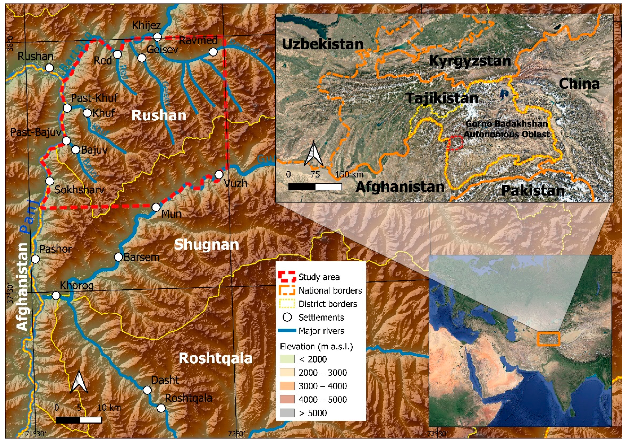
2.1. Study Area

The study area covers 1280 km2 of the western part of the Rushan Range in the Western Pamirs of Tajikistan (Figure 2). Administratively, it belongs to the Rushan and Shugnan districts of the Gorno-Badakhshan Autonomous Oblast (i.e., Province; GBAO). It is delimited by the river Gunt in the south, the river Panj in the west, the river Bartang in the north, and the 72°E meridian in the east. The highest peaks reach more than 5000 m a.s.l., while the minimum elevation is found in the northwestern corner at 1980 m a.s.l. The harsh climate is characterized by severe, long winters with minima below −35 °C, followed by short summers. The annual mean temperatures range between −7.1 °C on the Fedchenko Glacier and 8.7 °C at the meteorological station in the region’s center in Khorog [51,92,93,94]. Breckle [94] reports an annual precipitation in the Western Pamirs of between 90 and 400 mm, with a distinct winter maximum. This region is also part of the upper watershed of the Amu-Darya, rendering it crucial for the water supply for millions of people living downstream [95]. The Western Pamirs are considered to be a biodiversity hotspot [48,49,51,96,97], and large parts of it are (though insufficiently) protected by the Tajik National Park [98,99,100]. Around 2000 vascular plant species, including 160 endemics and a high number of threatened animal species, such as the snow leopard (Panthera uncia) and the Marco Polo sheep (Ovis ammon polii), are native to this area [49,101]. Furthermore, numerous wild progenitors of cultured fruit trees are found in the region, constituting a valuable genetic resource [50,93,96]. The Western Pamirs are also the habitat of rare juniper forest patches and Tugai forests (azonal forests in river valleys), which play important roles in the water regulation of rivers. Moreover, a large number of endemic dwarf shrub species dominate the upper vegetation belts. Further information on the vegetation in the study area is provided in Section 2.2.5.

2.2. Data

We collected Landsat images of the study area and built a raster time series of the modified soil adjusted vegetation index (MSAVI; 2.2.1). Additionally, we gathered time series of temperature and precipitation (2.2.2), population (2.2.3), and livestock data (2.2.4). Furthermore, we used the vegetation and land cover data of a historic Soviet vegetation map and ground-truthing records from fieldwork (2.2.5), as well as topographic variables derived from the shuttle radar topography mission (SRTM) digital elevation model (DEM; 2.2.6).

2.2.1. Landsat Data

We used the Earth Resources Observation and Science (EROS) Center Science Processing Architecture (ESPA) on demand interface (https://espa.cr.usgs.gov/, accessed on 6 July 2020) provided by the United States Geological Survey (USGS) to obtain pre-processed satellite scenes and derived the MSAVI [71] from the Level-2 Surface Reflectance [103] of the sensors Landsat 5 TM, Landsat 7 ETM+, and Landsat 8 OLI with a spatial resolution of 30 m. The calculation formula of the MSAVI is as follows:
MSAVI = 2 ρ N I R + 1 ( 2 ρ N I R + 1 ) 2 8 ( ρ N I R ρ r e d ) 2
where ρ N I R is the surface reflectance of the near-infrared band and ρ r e d is the surface reflectance of the red band.
Furthermore, a cloud and cloud shadow mask was calculated according to the CFMask algorithm [104,105,106]. Altogether, we obtained 1267 scenes of the study area between 1988 and 2020, which we combined in a 32-year raster image time series.

2.2.2. Climate Data

We used the 2-m air temperature and precipitation data from three different data sources. Daily climate data were obtained from the meteorological station in Khorog, located in the Panj valley at 2084 m a.s.l. The data were downloaded from the Climate Data Online (CDO) archive of the National Centers for Environmental Information [107]. Furthermore, we utilized reanalysis data from the European Centre for Medium-Range Weather Forecasts (ECMWF) Reanalysis v5-Land (ERA5-Land) dataset with a spatial resolution of 0.1° [108], and the Modern-Era Retrospective analysis for Research and Applications version 2 (MERRA-2) dataset with a spatial resolution of 0.5° × 0.625° [109], as these products proved to be the most suitable for vegetation analysis in mountain regions with limited data availability [110].

2.2.3. Population Data

Since the demographic development of a given region is a critical factor for both its use of resources and its potential to originate labor force for cultivation, we included the time series of population numbers in GBAO in our analysis. We combined two sources published by the State Agency for Statistics under the President of the Republic of Tajikistan (TajStat, [111,112]) in a 28-year time series (1990–2018) for the entire GBAO and in a 25-year time series (1990–2015) for the individual districts.

2.2.4. Livestock Data

For the discussion of grazing impact on the development of land cover and vegetation, we used numbers of large livestock (i.e., mainly cattle) collected by TajStat [113,114,115], which differentiate between the entire GBAO and each district. A consistency check of the data revealed that the time series could not be completely combined, as the numbers in the oldest dataset (1981–1996) are three times lower than the numbers in the two other datasets (1992–2011). Therefore, we decided to aggregate only the latest two of the datasets and analyze the resulting two time series separately from each other.

2.2.5. Vegetation and Land Cover Data

To evaluate the results of the MSAVI trend analyses, we used a historical vegetation map produced by the Soviet botanist Okmir Agakhanjanz in 1958–1961 (see [97] for details), which distinguishes between 12 different vegetation and land cover classes in the study area (Table 1). Additionally, to check the information from the maps and the results of the trend analyses for plausibility, we recorded 76 ground-truth field plots all over the study area.

2.2.6. Topographic Data

We evaluated relationships between the trends and topography using six topographic variables derived from the SRTM DEM with a resolution of 1 arc-second (30 m) [102]. Elevation was directly extracted from the DEM and used as the basis to calculate the slope, aspect, ruggedness, and distance to the valley bottom using the function terrain of the R package raster [116]. The aspect was transformed into north and east exposedness by calculating the cosine and sine of aspect, respectively [117].

2.3. Time Series Analysis Using Generalized Additive Mixed Models

Generalized additive mixed models (GAMMs) [86,118] were applied as an innovative approach that has rarely been used in remote sensing studies, using the function ‘gamm’ of the R package ‘mgcv’ [119]. Depending on the type of time series used, our response variables were MSAVI, temperature, precipitation, population, and livestock numbers, respectively. Their expected values were estimated by the explanatory variable ‘year’. We additionally included the explanatory variables ‘day of the year’ for the MSAVI time series and the variable ‘month’ for the temperature and precipitation time series. In doing so, we were able to separate the seasonal from the inter-annual component and hence could uncover gradual as well as abrupt land cover changes. In contrast to seasonal changes, which are mostly dependent on annual temperature and rainfall interrelations altering plant phenology, gradual changes can be caused by inter-annual climate variability or land degradation and land management. Abrupt changes are usually caused by disturbances and extreme events.
Due to the different periods and spatial scales at which the different response variables operate, the trend comparisons had to be limited to qualitative discussions.
GAMMs are extensions of generalized additive models (GAMs; [120]) and, as such, are able to estimate non-linear trends. They are a preferred method for ecological studies since they allow for complex shapes of response and are well-suited to cope with irregular spacing in a time series. Similar to other regression models, in a GAMM, a univariate response variable is related to one or multiple explanatory variables. As in generalized linear models (GLMs; [121]), the mean of the response variable in GAMMs is related to the explanatory variables by a link function. However, as opposed to parametric models, GAMMs make use of smoothing functions of the explanatory variables. The resulting smoothing curves can take on many forms and allow for non-linear relationships between the response and explanatory variables [66]. The general equation of a GAM is:
g(μ) = ∑f(X),
where g is a specified link function, (μ) is the expected mean response, and ∑f(X) is the smooth functions of the covariates (X). In GAMMs, a random factor is added to this general GAM equation. For a detailed description, readers are referred to Wood [86].
In this study, we used a Gaussian distribution and two types of smoothers—i.e., (1) thin plate regression splines for the development of the data values over the years and (2) cyclic cubic splines to account for the seasonality in the MSAVI, temperature, and precipitation data. The value of the smoothness parameter had to balance between a model that was too simple to sufficiently represent the data and an exceedingly complex model that overfitted the data. With this in mind, the degree of smoothness was optimized by treating it as a random effect using the maximum likelihood method [65,86,122]. As the values in our time series are mostly irregularly distributed in time, we introduced a continuous-time first-order autoregressive process (CAR(1)) to account for autocorrelation in the data that may bias the trend results [65,118]. To compensate for differences caused by the sensors, which may otherwise distort the trend results, we used ‘sensor type’ (a factor variable with the three levels Landsat 5 TM, Landsat 7 ETM+, and Landsat 8 OLI) as a random effect (random intercept and random slope) variable in the GAMM models for the analyses of the MSAVI time series [86].
We applied the GAMM function to each time series, and this approach allowed us to address the time, amount, and direction of change within the trend component. For the MSAVI time series, we present significance and amount of change as a map (Figure 3). In doing so, the detected changes were localized on the vegetation map and subsequently further evaluated. In particular, for the 1200-pixel time series, we conducted further statistical analyses to obtain deeper insights into the development of the land cover. These 1200 comprise 100 time series for each of the 12 land cover types. Seventy-six of these locations were visited in the field, giving us a better understanding of the on-site situation. The remaining 1124 locations were stratified randomly and selected using the function ‘stratified’ of the R package ‘fifer’ [123].
Furthermore, we identified points of significant change in the time series. In contrast to linear models, where each point in the time series always has the same slope of the trend, in non-linear models, such as GAMMs, each time point may have a different slope. To solve this difficulty, we estimated the first derivative of the fitted splines by calculating finite differences for numerous time points in the time series [65]. Then, we evaluated if the first derivatives at these time points comply with the null hypothesis of no change. This was achieved by calculating a 95% confidence interval for the derivative estimates. Points in the time series where zero is outside the confidence interval of the first derivative indicate times of significant change. For a detailed description of this method, readers are referred to Simpson [65].

3. Results

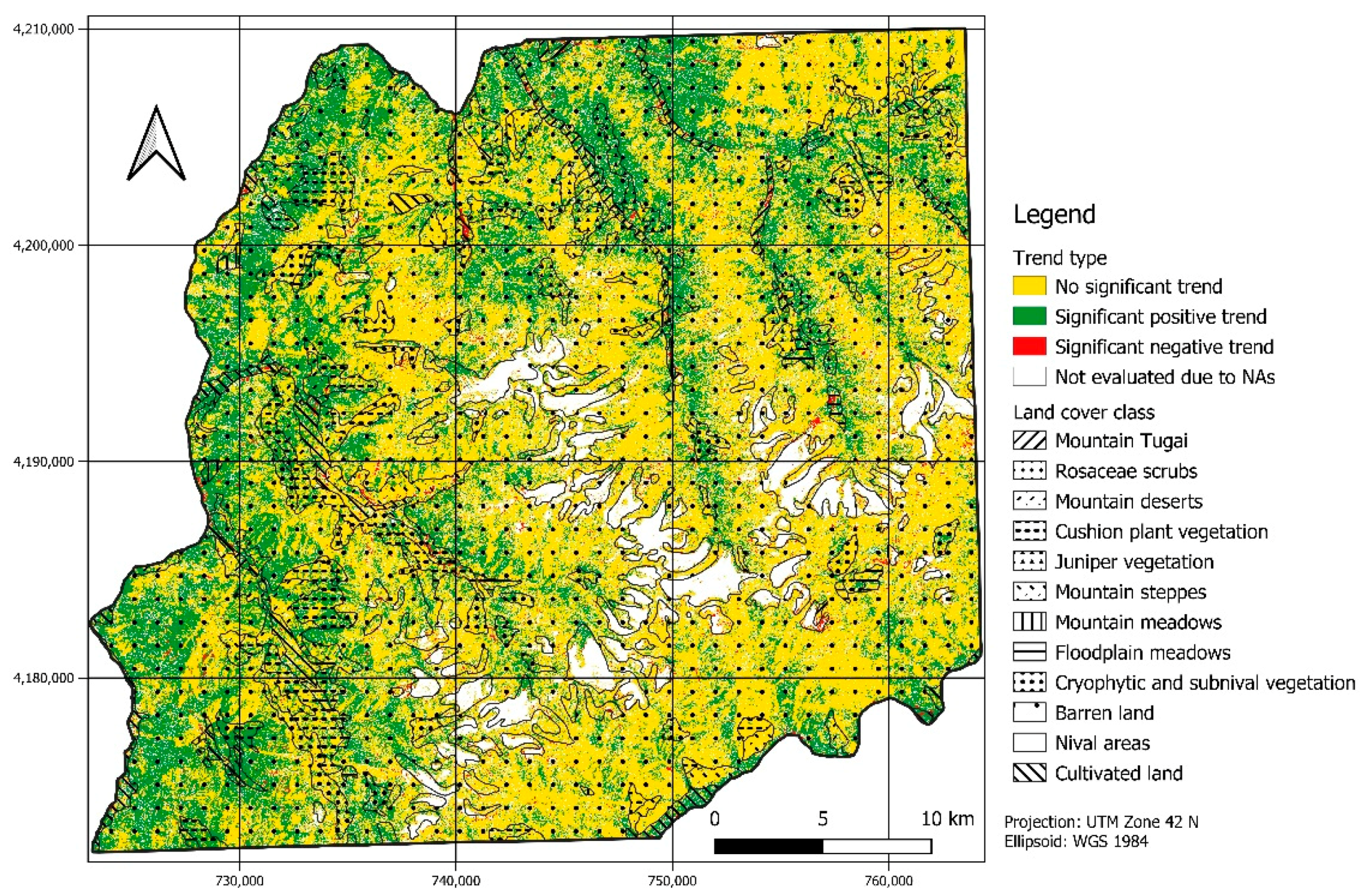
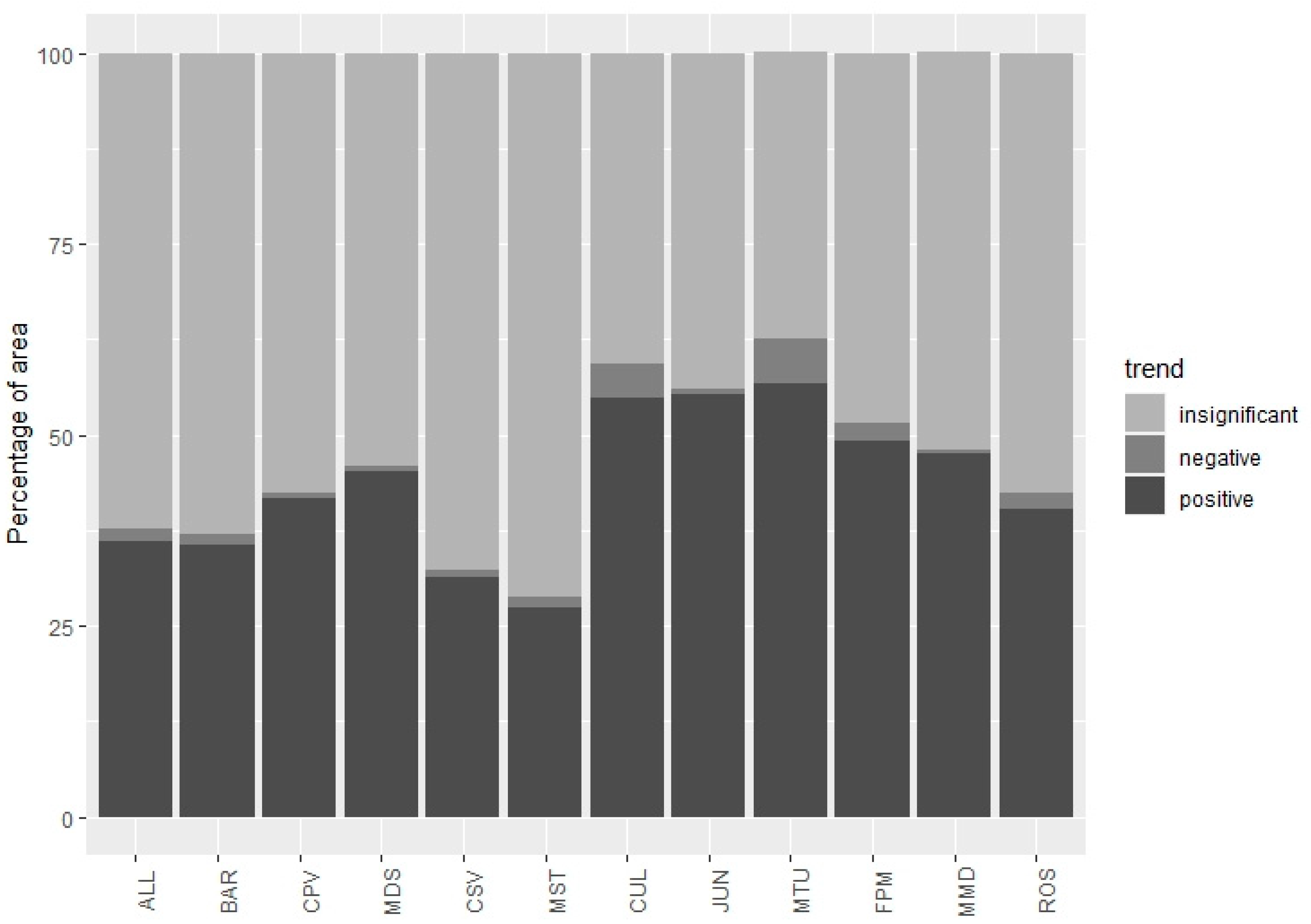
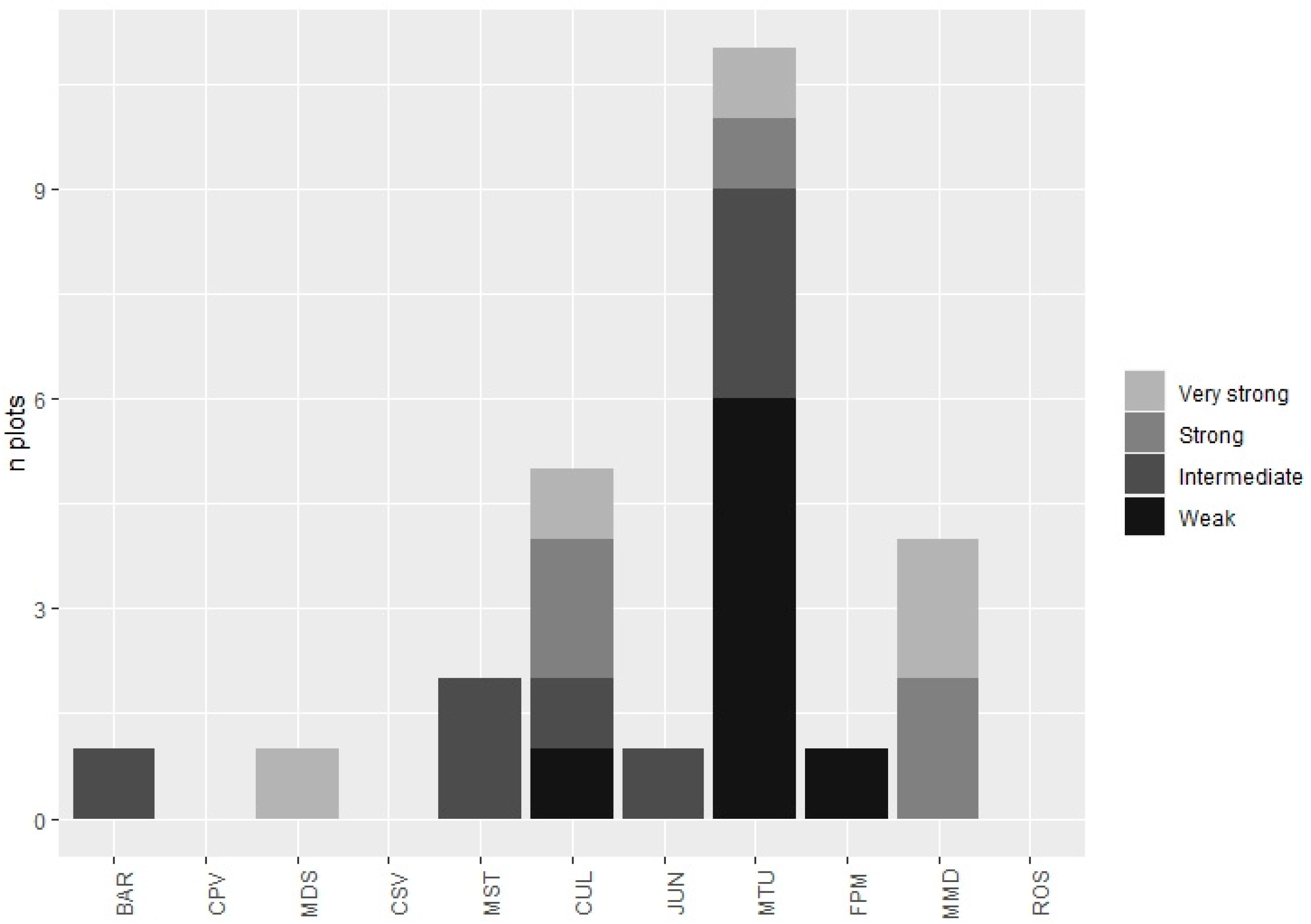
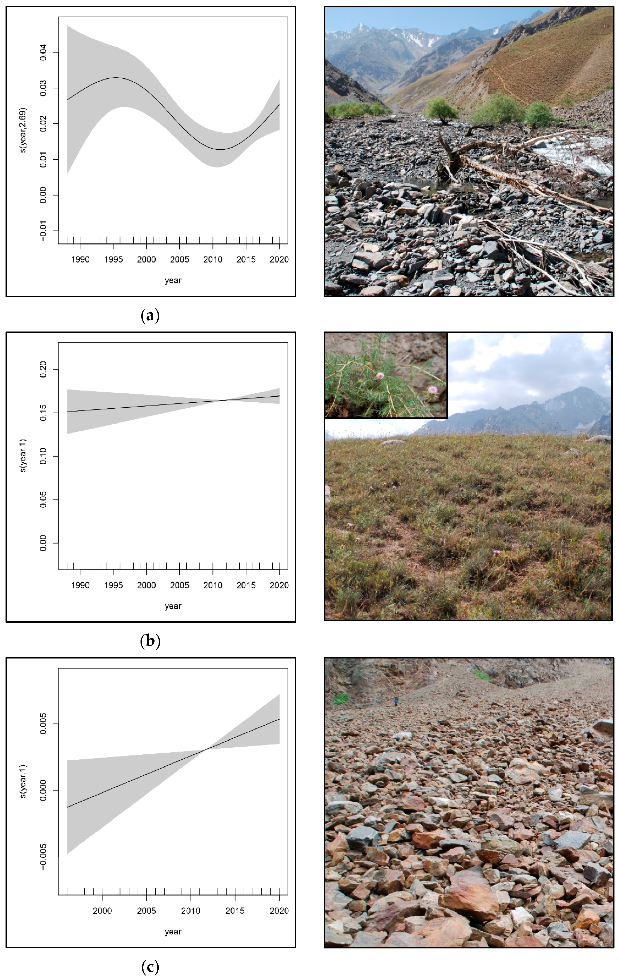
3.1. Vegetation Greening and Browning Trends as Indicated by MSAVI Time Series

In this study, we refer to a significant positive (i.e., increasing) trend of MSAVI values over the study period (1988–2020, p < 0.05) as greening, whereas a significant negative (i.e., decreasing) trend (1988–2020, p < 0.05) is called browning. In total, we analyzed more than 1.4 million pixel time series of an area of 1280.2 km2. For 16.5% of these time series, there were too few observations to perform statistical analyses. In the remaining time series, we detected greening for 385.9 km2 (36.1%). In contrast, only 17.2 km2 (1.6%) showed browning. The majority of the time series (62.3%, 666.5 km2) did not exhibit a significant trend (p > 0.05) of MSAVI increase or decrease (Figure 4).
A visual evaluation of the trends suggests that the time series with no significant changes are distributed all over the study area and, in particular, on slopes, ridges, and high plateaus. Greening could be detected predominantly in the western part of the study area—i.e., in Panj and its adjacent valleys, along the valleys of Bartang in the north, its tributary valleys Geisev in the north-central, and Ravmed in the northeast—and in Gunt Valley in the south of the study area. Time series with significant browning are partly clustered in valley bottoms, with the biggest area located in Red Valley in the northwest of the study area. The parts of the study area with too few observations for meaningful statistical analyses predominantly belong to the nival areas with a permanent snow or ice cover across the entire year (Figure 3).
This visual evaluation was supported by a quantitative analysis, which revealed that trend types of the land cover classes, to some extent, differ fundamentally from the situation in the entire study area and from each other (Figure 4). In four classes (mountain Tugai, juniper vegetation, mountain meadows, and cultivated land), the number of time series with significant greening exceeds the number of time series with no trend. The share of time series with significant browning is particularly high in mountain Tugai and cultivated land. Time series with no significant trend dominate, especially in mountain steppes and cryophytic and subnival vegetation. Nival areas also show a large proportion of browning and no significant change. However, the very low number of valid observations in these time series suggests spurious trends. Therefore, we decided to refrain from further interpretation.
In the next step, we deepened the analysis based on the characteristics of 1100 test time series, with 100 from each land cover class (except nival areas). First, we examined whether the single years showed significant greening, significant browning, or no significant change. We ascertained that 55% have no significant change in each of the 32 analyzed years. In 36.7%, MSAVI increased significantly in all years—i.e., we detected a continuous linear trend over the entire study period. A continuous browning trend was revealed for less than 1% of the time series. Non-linear shapes—i.e., a mix of greening, browning and insignificant change over the years—were found for 7.7% of the time series. However, the individual land cover classes partly exhibit considerable differences from this result (Table 2). Non-linear time series occur predominantly in mountain Tugai (19%) and cultivated land (16%). Another remarkable land cover class is the mountain steppes. They have the highest proportion of no change in all the years (76%), followed by cryophytic and subnival vegetation (63%). Constant greening over the entire study period was especially detected in juniper vegetation (46%) and Rosaceae scrubs (46%), followed by barren land (43%).
Then, we compared the amount of change—i.e., the difference in MSAVI of the component smooth functions for the variable ‘year’ between 1988 and 2020 and between the different types of times series based on their median values: for all non-NA time series, the median is 0.01, for time series with a significant greening trend it is 0.02, and for time series with a significant browning trend it is −0.03 (Table 3). To put these rather small values into perspective, we need to consider that the median MSAVI calculated over all 1100 test plots for the whole time series is only 0.06. The comparison of the absolute values did not unveil patterns of change between the land cover classes. In such cases, a common approach is to compare the classes in terms of some measure of location [124,125]. We calculated the quartiles that are standard statistical location parameters to compare the differences between land cover in the four different categories in terms of the amount of change, as described below.
First, we calculated the quartiles of all change values in the test plots with a significant positive change (n = 486). We call values above the 75% quantile a ‘very strong change’, values above the median but smaller than the 75% quantile ‘strong change’, values above the 25% quantile to the median ‘intermediate change’, and values below the 25% quantile ‘weak change’. Then, we compared the land cover classes based on their share of change values in the four categories (Figure 5). In particular, cultivated land has many plots with a very strong positive change, followed by mountain deserts. Mountain meadows is the land cover class with the highest number of plots with strong positive change, followed by floodplain meadows. The category intermediate change is led by juniper vegetation, followed by Rosaceae scrubs. Plots with weak positive change are predominantly found in juniper vegetation, followed by mountain Tugai and barren land.
Analogous to the plots with a significant positive change, we calculated the quartiles of the modulus of the change values in the test plots with a significant negative change (n = 26). Again, we compared the land cover classes based on their share of change values in the four categories (Figure 6). There are no plots with a significant negative change among Rosaceae scrubs, cushion plant vegetation, and cryophytic and subnival vegetation. The highest number of negative changes was found in mountain Tugai, though most plots fall into the category of weak negative change. Very strong and strong negative changes predominantly occur in mountain meadows, followed by cultivated land.
With regard to topography, we found significant differences (p < 0.05, Mann–Whitney U-test) between the trend types for all analyzed variables (Table 4). Regarding elevation, there is a significant difference between all three trend types, with the highest values discovered for time series with a significant browning trend, followed by time series with no significant trend and time series with a significant greening trend. The slope values also differ significantly between the three trend types, with the steepest slope for time series with significant greening, followed by time series with no significant trend and time series with significant browning. Furthermore, the time series of the three trend types differ in terms of their north exposedness. The highest values could be detected for time series with a significant browning trend, followed by time series with a significant greening trend and time series with no significant trend. Moreover, the time series of the three trend types show a significantly different east exposedness. The highest values appear in time series with no significant trend, followed by time series with a significant browning trend and time series with a significant greening trend. Considering the ruggedness of the terrain, we also found significant differences between the time series of the three trend types, with the highest values for greening time series, followed by no trend time series and browning time series. Greening time series are the trend type closest to valley bottoms, followed by browning time series and no trend time series.
Finally, with regard to the geographic position as indicated by Universal Transverse Mercator (UTM) easting and northing, we also detected significant differences between all three trend types. For UTM easting, the highest values occur in browning time series, followed by no trend and greening time series. Regarding UTM northing, the values of greening time series are significantly higher than the values for no trend and browning time series, neither of which differ from each other.

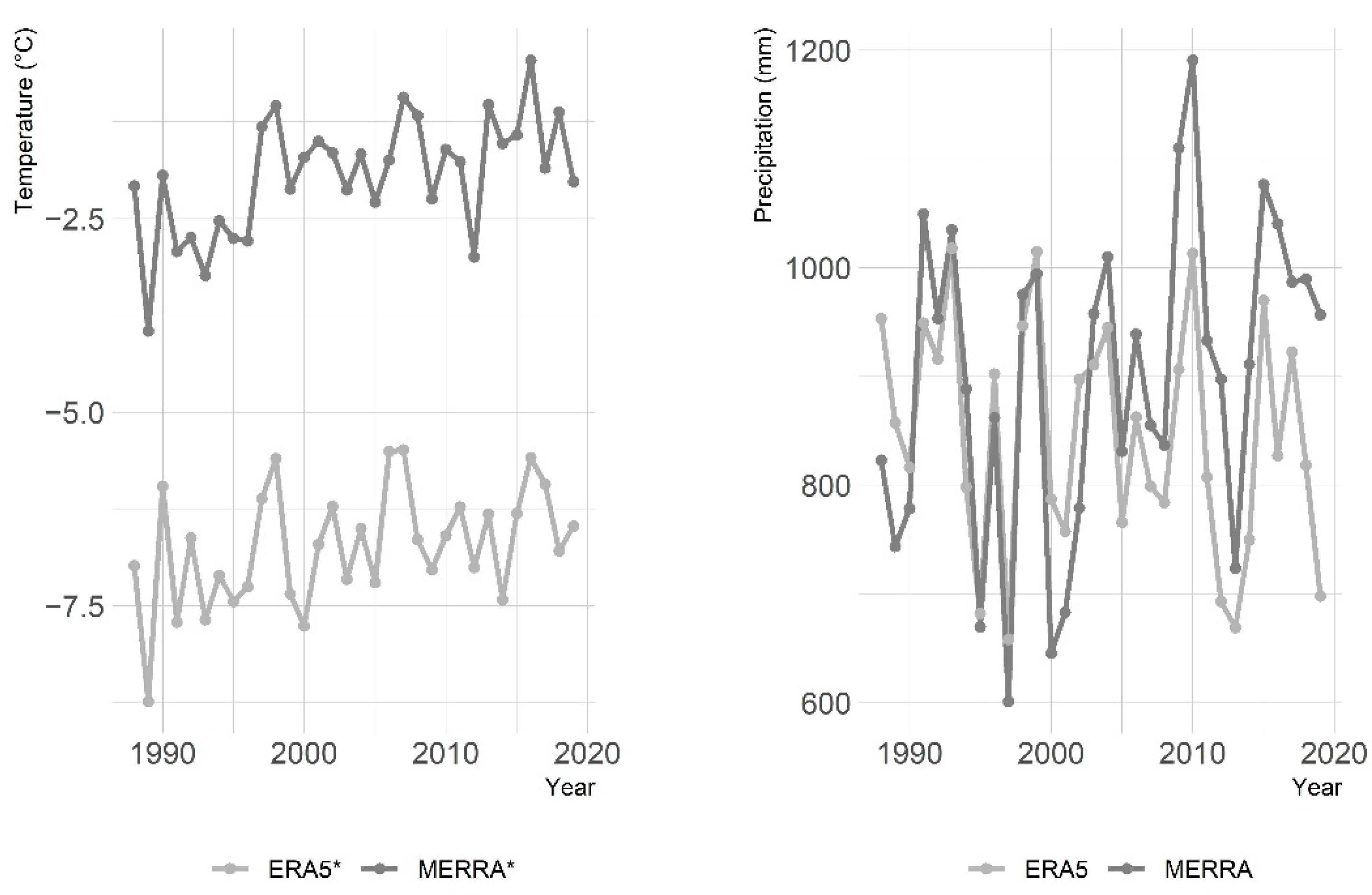
3.2. Trends of Temperature and Precipitation

The visual inspection of the ERA5 and MERRA annual mean temperature values shows increasing trends for both time series (Figure 7 left). This observation is supported by the results of the GAMMs, where the component smooth functions of the variable ‘year’ revealed a significant (p < 0.01) increasing trend from 1988 to 2020 for all three analyzed temperature time series (CDO Khorog, ERA5, MERRA). The CDO time series, however, has many missing values; therefore, its result should be interpreted with caution, and meaningful annual means could not be calculated and plotted. The biggest temperature increase of 1.45 °C over the study period was indicated by the MERRA time series, followed by the ERA5 time series with 0.95 °C and the CDO time series with 0.8 °C.
In contrast, we could not find consistent trends in the precipitation data (Figure 7 right). The results of the GAMMs for the ERA5 and MERRA time series also support the assumption of no significant change over the study period (p > 0.05). Only the GAMM for the CDO precipitation data of the meteorological station in Khorog exhibits a significant increase in precipitation after 2007. However, this result is influenced by many missing values before this date.

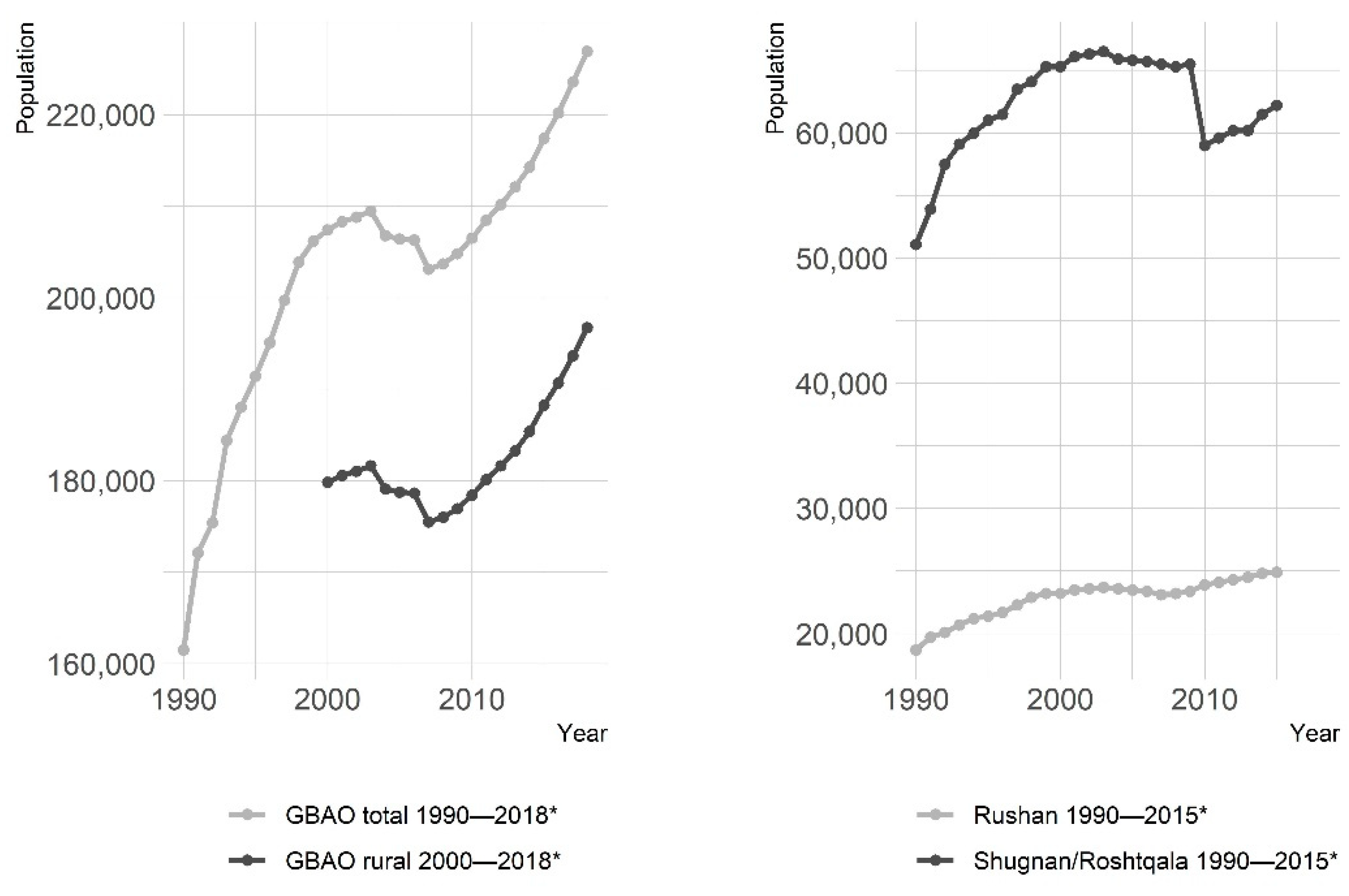
3.3. Trends of Population Development

The population in the study area and its surroundings increased during the study period (Figure 8). This is visible in the time series for the entire GBAO from 1990 to 2018, including the city of Khorog, and for the rural population (2000–2018). The numbers steeply increased until 2001, then slightly decreased from 2003 to 2007, and finally further increased after 2008. The smooth functions in the GAMMs confirm a significant (p < 0.01) positive trend. The population numbers (1990–2015) in the districts of Rushan, where the major part of the study area is located, and Shugnan/Roshtqala, the district of the southern part of the study area, show a positive trend as well. Rushan’s population significantly increased until 2001, then remained stable, and lastly slightly increased after 2006. In Shugnan/Roshtqala, the numbers increased strongly until 2000, then remained stable on a high level, declined in 2010, and again increased in recent years.

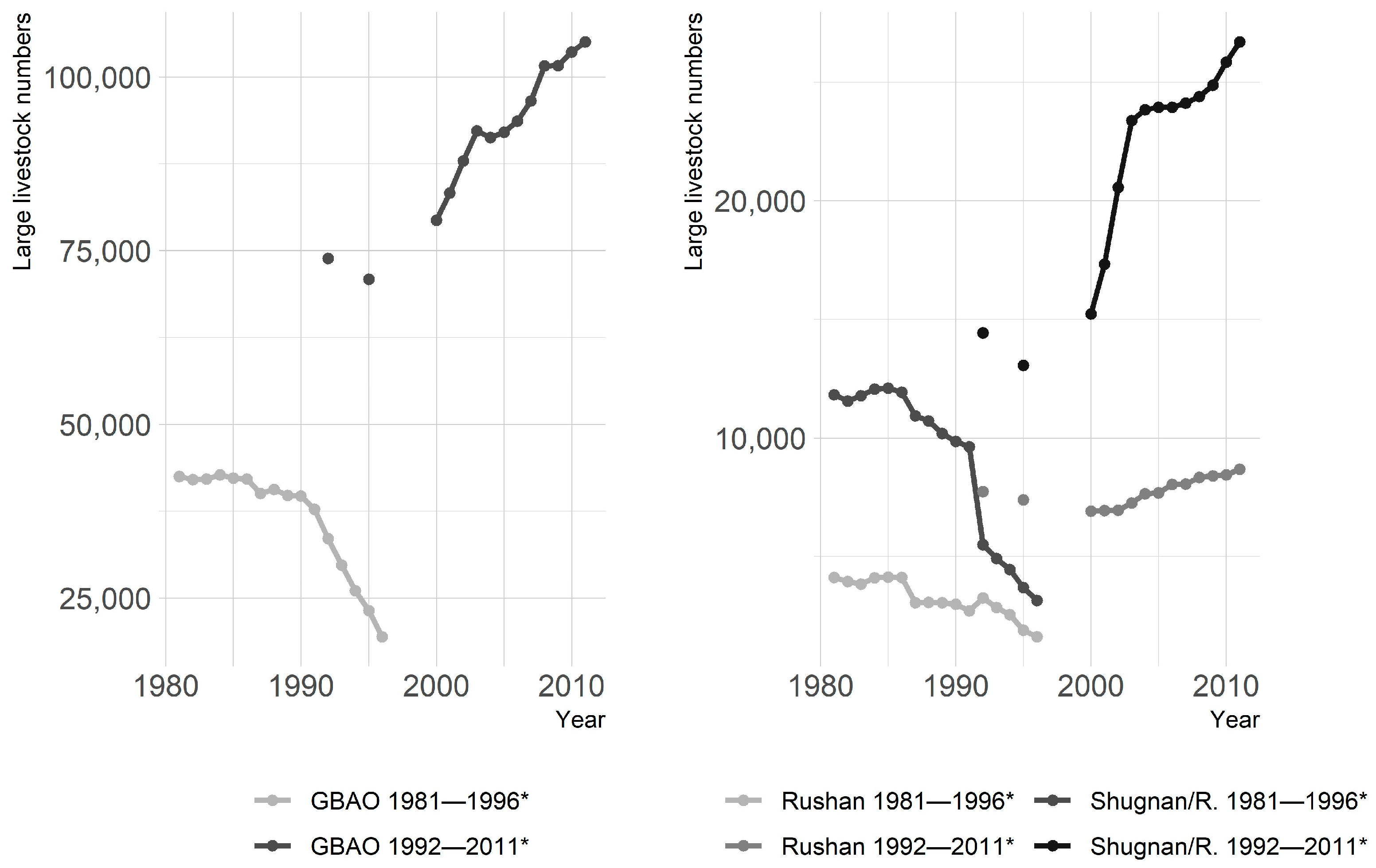
3.4. Trends of Large Livestock Numbers

The numbers of large livestock in the study period first sharply decreased, at least until 1996, but exhibited a strong increasing development after 2000 (Figure 9). The time series for the entire GBAO from 1981 to 1996 shows stable numbers of around 42,000 large livestock heads until the end of the 1980s, followed by a significant (p < 0.01) decrease until 1996 to 19,440 animals. The GBAO time series from 1992 to 2011 exhibits a significant (p < 0.01), near linearly increasing trend from 2000 to 2011. While the numbers stay below 80,000 in the 1990s, 105,011 animals were counted in 2011. The decline in the livestock numbers at the beginning of the 1990s was also detected in the time series of the districts of Shugnan/Roshtqala and Rushan, where the numbers decreased from 11,814 to 3136 and from 4113 to 1610, respectively. The increase from 6904 to 8677 animals in Rushan after 2000 appears rather flat in the visualization but is nevertheless significant (p < 0.01). For Shugan/Roshtqala, we detected a significant steep increase from 2000 to 2003, followed by a further moderate increase.

4. Discussion

To our knowledge, this is the first study that successfully uses GAMMs to analyze vegetation and land cover change with a raster time series in complex dry mountain terrain. By combining this approach with a relatively long Landsat time series and a particularly suitable vegetation index, we addressed several common challenges of applied remote sensing studies in dryland mountain regions, such as irregular data, high background influence, and non-linearity.

4.1. Detection of Greening and Browning Trends

The analysis of the 32-year pixel-based MSAVI time series revealed significant land cover changes in about 40% of the study area from 1988 to 2020. Concerning the direction of change, the area exhibiting a greening trend by far exceeds the area with a browning trend. This finding coincides well with observations on a global scale, where trends of increasing green vegetation cover were detected in many regions of the world in recent decades [3,4]. About 60% of the analyzed area showed no significant land cover change.

4.2. Distinction of Greening and Browning Trends

We detected greening in all land cover classes, though the largest proportions were found in areas at or near the valley bottom. The amount of change was highest in cultivated areas. This finding is not in line with our expectation that valley bottoms are characterized mainly by browning due to overuse [49,51,59,63]. The highly elevated land cover classes show a smaller percentage of greening; however, due to their large extent, the absolute areas are still extensive. Cryophytic and subnival vegetation have a high proportion of time series without significant change, which shows the stability of this high-elevation land cover class. This is also an unexpected finding, as it contradicts the results of other studies that expect greening, particularly in the highest altitudes [43,44,126].
Browning could be detected for less extensive areas, though it also occurred in all land cover classes and predominantly in vegetation at or near the valley bottom. These time series mostly show a non-linear development, indicating abrupt changes. A cluster of such non-linear negative development was found in Red valley in the northwest of the study area, which resulted from a debris flow in 2011 (Figure 10a).
For the variable slope, browning sites have the lowest median, which can be explained by the highest impact of disastrous events in the relatively weakly inclined valley bottoms, whereas greening was detected in both steep and flat areas. The same explanations hold true for north-exposedness, for which the median in sites with browning is the highest. Again, this is because a relatively large cluster of browning was found in a north-exposed valley. However, we assume that north-exposedness is not a general explanation for browning trends, as similar events also occurred in south-exposed valleys outside the study area—e.g., around the village of Barsem [94,127].

4.3. Relationship of Greening and Browning Trends to Temperature and Precipitation

For mountains, in particular, rising temperatures and a prolonged growing season were discussed as major drivers for increasing vegetation cover and species richness in alpine areas. As the temperature is one of the major limits on plant growth, warming reduces this constraint [43,44,128]. For the study area, we found significantly rising temperatures. This result is in line with the findings of Haag et al. [129,130]; the review of Robinson [59]; δ18O data from ice cores [131]; and the Intergovernmental Panel on Climate Change (IPCC) report, which expects an increase of 3.7 °C in the mean annual temperature (temperature change for 2080–2099 in comparison to 1980–1999) in the region [132]. We conceive these results as a strong indication that warming also plays a role in the greening of the study area. In most of the pixel time series that exhibit a greening trend, the increase in MSAVI is linear. This finding corresponds well to the nearly continuous temperature increase and corroborates the role of rising temperatures as a driver of greening. In arid areas, increasing precipitation is a frequent driver of greening [6,11]. However, we did not find significant trends of change in precipitation for the study area. This result is backed by the findings reviewed by Robinson [59], whereas Deji et al. [131] found a wetting trend in δ18O ice core data, and Haag et al. [129] detected increased summer precipitation.
In the highly elevated land cover classes, the increasing temperature that causes permafrost thawing is likely to contribute to the observed greening, particularly in moraine material that is classified as barren land, as well as in cryophytic and subnival vegetation. Peng et al. [133] investigated permafrost–vegetation relationships in the northern hemisphere and were able to show that the increased number of thawing days prolongs the growing season and increases the active layer thickness, which facilitates vegetation growth in permafrost regions. In the Pamirs, this is an important point, as 84.1% of the GBAO was identified as a potential permafrost area. Projections based on a scenario of a temperature increase of 4 °C until the end of the century expect a disappearance of 40% of the recent permafrost areas in the GBAO [134].
Furthermore, thawing permafrost decreases slope stability and hence promotes gravitational mass movements. Together with increased run-off induced by intensified melting of snow and glaciers [135,136,137,138,139], this may create catastrophic mass flows that devastate the valley bottoms and thus lead to an abrupt browning signal in remote sensing data [127,134,140]. Indeed such events of gravitational mass movement regularly occur in high mountains [127,140]. However, the prospective consistent temperature increase within the next few decades [132] will accelerate such events. Additionally, heavy summer rains in the study area in recent years resulting from disturbances triggered by the Indian Summer Monsoon or originating from extratropical cyclones [139,141,142,143] exacerbate these processes. In some cases, the enhanced melting can lead to the development of glacial lakes and subsequently to glacial lake outburst floods (GLOFs). Such an event occurred in Shakhdara valley, ca. 50 km south of the study area, where a GLOF destroyed the village of Dasht in 2002, killing dozens of people and devastating vegetation [127,134].

4.4. Relationship of Greening and Browning Trends to Population and Livestock Numbers

The strong greening trend of the land cover classes at and near the valley bottom can be explained by the increased cultivation efforts of a rising population size together with improved land management practices linked to privatization since the breakdown of the Soviet Union [59]. Another argument in favor of this explanation is that most of the greening areas are located in regions where the highest population numbers are reported. Furthermore, the restoration and extension of irrigation systems are likely to play important roles. After a major extension of these systems during the Soviet period, their maintenance ceased with independence. However, many of these systems have been reestablished—e.g., as community-based irrigation governance systems (see, e.g., [144]). Similarly, projects of joint forestry management have helped to restore the Tugai scrubs and forests [145].
In mountainous drylands, floods and debris flows are often disastrous, as arable and irrigation lands, as well as associated villages, are predominantly situated on narrow river terraces and alluvial plains in valley bottoms [144]. In this area, the Tugai scrubs and forests play the dominant role in river discharge regulation and embankment stability, as well as in the protection of soils and infrastructure. Directly after the Soviet breakdown, these forests strongly degraded because of the energy crisis that forced the local population to use the Tugai for fuelwood and timber, leading to the increased vulnerability of the valley vegetation, arable land, and local communities [144,145,146,147,148]. In some areas, the state of these forests has already improved, but there is still an increased vulnerability to natural disasters in many areas due to poor forest conditions [149].
Another factor considered to be an important driver in browning is grazing impact. Our results show that the livestock numbers in the study area declined after the Soviet breakdown but strongly increased in the last two decades. This finding coincides with the results of Robinson [59]. Furthermore, current trends towards a reduction in livestock mobility and the abandonment of remote pastures are causing overgrazing in easily accessible areas and, in particular, around villages [59,62,150]. The increasing livestock numbers are primarily driven by the increasing population that we found for GBAO since 1990. In particular, the outbreak of the Tajik civil war in 1992 is seen as an important booster initiating the rising numbers after the Soviet breakdown [63]. A higher population also increases the need for other natural resources, such as fuelwood and timber. In the study area, the Tugai forest is the most important provider for these ecosystem goods, which explains the browning trend seen in some parts of this land cover class.
Indeed, we detected browning in land cover classes extensively used for grazing livestock—e.g., in meadows—though the extent is low. Mountain steppes, another heavily grazed land cover class, exhibit the largest proportion of pixel time series without significant change (for an illustration, see Figure 10b).
According to our observations, grazing caused no changes in vegetation quantity here but rather in vegetation quality. An explanation can be found in the long grazing history of the study area and the change to vegetation dominated by prickly shrubs and herbs or plant species that contain alkaloids [96,151]. Our field data support these findings. For example, we found many unpalatable species, such as Senecio spp., and we frequently detected a strong dominance of prickly herbs—in particular, of the genus Cousinia—in areas where historical vegetation studies reported a much lower quantity of this plant type [97]. We conclude that the change in the mountain steppes is not visible in the remote sensing data but is evident on species and trait levels.
The inspection of 76 ground-truthing sites in the field and comparison with the historic vegetation map support the plausibility of the findings derived from the remote sensing analyses in most cases. However, the results for scree sites with no vegetation should be interpreted with caution, as we detected unreliable steep positive trends in some rare cases (see the example given in Figure 10c).

5. Conclusions

In this paper, we presented an innovative and promising approach for analyzing land cover trends in dry mountain systems by combining long-term Landsat image time series with environmental and socio-demographic data using GAMMs. Thereby, we were able to tackle several challenges of remote sensing studies in mountainous drylands, such as irregular data, high background influence, non-linearity, and sensor issues. We found that greening and browning trends coexist in the study area, with greening being predominant. The characteristics of the detected trends vary according to the vegetation and land cover classes involved, as well as their topographical and geographical distribution. With the applied approach, we were able to detect remarkable changes at a small spatial scale—e.g., in narrow valley bottoms that remained undetected in previous long-term remote sensing studies. These areas are predominantly used for agriculture and forestry, which suggests direct anthropogenic drivers of change here. We also discovered a high number of pixels with a greening trend that corresponds well with increasing temperature. Trends of increasing precipitation, which would support greening, were not observed. Detected browning was mainly attributed to disastrous events that were most probably enhanced by increasing temperatures. Contrary to our expectations, browning trends did not correspond well with an increasing population and increasing livestock numbers. Grazing increased, but associated changes were not detectable with our approach. This can be explained by our field observations, which showed that the respective effects are most active on the species and trait level. Different approaches and future studies are required in order to enhance our understanding of the processes involved at this resolution. Nevertheless, this study presents trends of land cover change in the Pamir mountains with a novel methodology that could serve as a basis for further research on vegetation dynamics for management purposes—e.g., for sustainable pasture and forest management. Thereby, the approach shows high potential in mountainous and dry areas globally.

Author Contributions

K.A.V. designed the study, conducted the analysis, and wrote the manuscript; H.Z. and C.S. revised the manuscript; K.A.V., H.Z. and C.S. discussed the results and reviewed and edited the manuscript. All authors have read and agreed to the published version of the manuscript.

Funding

This research was funded by the Belmont Forum, the German Research Foundation (grant numbers SA 775/12-1 and VA 749/4-1), and the Schmauser Foundation.

Institutional Review Board Statement

Not applicable.

Informed Consent Statement

Not applicable.

Data Availability Statement

Not applicable.

Acknowledgments

The authors are grateful for the logistic support of this study by Saidmir Shomansurov (†), who sadly passed away in May 2020. We dedicate this study to his memory. Martin Häusser, Malte Manne, Matthias von Stackelberg, and Jakob Wernicke deserve thanks for supporting the data acquisition in the field. We also thank Andrei Dörre and Tobias Kraudzun for the provision and translation of population and livestock statistics. Furthermore, we would like to thank Ruth Tattershall, Christopher Dacosta, and Mattias Roth very much for language editing. Finally, we thank three anonymous reviewers for their time and effort in reviewing the manuscript.

Conflicts of Interest

The authors declare no conflict of interest. The funders had no role in the design of the study; in the collection, analysis, or interpretation of data; in the writing of the manuscript; or in the decision to publish the results.

References

  1. Pan, N.; Feng, X.; Fu, B.; Wang, S.; Ji, F.; Pan, S. Increasing Global Vegetation Browning Hidden in Overall Vegetation Greening: Insights from Time-Varying Trends. Remote Sens. Environ. 2018, 214, 59–72. [Google Scholar] [CrossRef]
  2. Nagendra, H.; Reyers, B.; Lavorel, S. Impacts of Land Change on Biodiversity: Making the Link to Ecosystem Services. Curr. Opin. Environ. Sustain. 2013, 5, 503–508. [Google Scholar] [CrossRef]
  3. Zeng, Z.; Peng, L.; Piao, S. Response of Terrestrial Evapotranspiration to Earth’s Greening. Curr. Opin. Environ. Sustain. 2018, 33, 9–25. [Google Scholar] [CrossRef]
  4. Zhu, Z.; Piao, S.; Myneni, R.B.; Huang, M.; Zeng, Z.; Canadell, J.G.; Ciais, P.; Sitch, S.; Friedlingstein, P.; Arneth, A.; et al. Greening of the Earth and Its Drivers. Nat. Clim. Chang. 2016, 6, 791–795. [Google Scholar] [CrossRef]
  5. Brandt, M.; Mbow, C.; Diouf, A.A.; Verger, A.; Samimi, C.; Fensholt, R. Ground- and Satellite-Based Evidence of the Biophysical Mechanisms behind the Greening Sahel. Glob. Chang. Biol. 2015, 21, 1610–1620. [Google Scholar] [CrossRef] [PubMed] [Green Version]
  6. Fensholt, R.; Rasmussen, K.; Nielsen, T.T.; Mbow, C. Evaluation of Earth Observation Based Long Term Vegetation Trends—Intercomparing NDVI Time Series Trend Analysis Consistency of Sahel from AVHRR GIMMS, Terra MODIS and SPOT VGT Data. Remote Sens. Environ. 2009, 113, 1886–1898. [Google Scholar] [CrossRef]
  7. Trichon, V.; Hiernaux, P.; Walcker, R.; Mougin, E. The Persistent Decline of Patterned Woody Vegetation: The Tiger Bush in the Context of the Regional Sahel Greening Trend. Glob. Chang. Biol. 2018, 24, 2633–2648. [Google Scholar] [CrossRef] [PubMed]
  8. Mueller, T.; Dressler, G.; Tucker, C.J.; Pinzon, J.E.; Leimgruber, P.; Dubayah, R.O.; Hurtt, G.C.; Böhning-Gaese, K.; Fagan, W.F. Human Land-Use Practices Lead to Global Long-Term Increases in Photosynthetic Capacity. Remote Sens. 2014, 6, 5717–5731. [Google Scholar] [CrossRef] [Green Version]
  9. Forzieri, G.; Alkama, R.; Miralles, D.G.; Cescatti, A. Response to Comment on “Satellites Reveal Contrasting Responses of Regional Climate to the Widespread Greening of Earth”. Science 2018, 360, 6394. [Google Scholar] [CrossRef] [PubMed] [Green Version]
  10. Lucht, W.; Prentice, I.C.; Myneni, R.B.; Sitch, S.; Friedlingstein, P.; Cramer, W.; Bousquet, P.; Buermann, W.; Smith, B. Climatic Control of the High-Latitude Vegetation Greening Trend and Pinatubo Effect. Science 2002, 296, 1687–1689. [Google Scholar] [CrossRef] [Green Version]
  11. Liu, Y.; Li, Y.; Li, S.; Motesharrei, S. Spatial and Temporal Patterns of Global NDVI Trends: Correlations with Climate and Human Factors. Remote Sens. 2015, 7, 13233–13250. [Google Scholar] [CrossRef] [Green Version]
  12. Brehaut, L.; Danby, R.K. Inconsistent Relationships between Annual Tree Ring-Widths and Satellite-Measured NDVI in a Mountainous Subarctic Environment. Ecol. Indic. 2018, 91, 698–711. [Google Scholar] [CrossRef]
  13. Jeong, J.-H.; Kug, J.-S.; Kim, B.-M.; Min, S.-K.; Linderholm, H.W.; Ho, C.-H.; Rayner, D.; Chen, D.; Jun, S.-Y. Greening in the Circumpolar High-Latitude May Amplify Warming in the Growing Season. Clim. Dyn. 2012, 38, 1421–1431. [Google Scholar] [CrossRef]
  14. Cho, M.H.; Yang, A.R.; Baek, E.H.; Kang, S.M.; Jeong, S.J.; Kim, J.Y.; Kim, B.M. Vegetation-Cloud Feedbacks to Future Vegetation Changes in the Arctic Regions. Clim. Dyn. 2018, 50, 3745–3755. [Google Scholar] [CrossRef]
  15. Silapaswan, C.S.; Verbyla, D.L.; McGuire, A.D. Land Cover Change on the Seward Peninsula: The Use of Remote Sensing to Evaluate the Potential Influences of Climate Warming on Historical Vegetation Dynamics. Can. J. Remote Sens. 2001, 27, 542–554. [Google Scholar] [CrossRef]
  16. Goetz, S.J.; Bunn, A.G.; Fiske, G.J.; Houghton, R.A. Satellite-Observed Photosynthetic Trends across Boreal North America Associated with Climate and Fire Disturbance. Proc. Natl. Acad. Sci. USA 2005, 102, 13521–13525. [Google Scholar] [CrossRef] [Green Version]
  17. Sturm, M.; Racine, C.; Tape, K. Increasing Shrub Abundance in the Arctic. Nature 2001, 411, 546–547. [Google Scholar] [CrossRef]
  18. Sturm, M.; McFadden, J.P.; Liston, G.E.; Chapin, F.S., III; Racine, C.H.; Holmgren, J. Snow-Shrub Interactions in Arctic Tundra: A Hypothesis with Climatic Implications. J. Clim. 2001, 14, 336–344. [Google Scholar] [CrossRef] [Green Version]
  19. Bhatt, U.S.; Walker, D.A.; Raynolds, M.K.; Comiso, J.C.; Epstein, H.E.; Jia, G.; Gens, R.; Pinzon, J.E.; Tucker, C.J.; Tweedie, C.E.; et al. Circumpolar Arctic Tundra Vegetation Change Is Linked to Sea Ice Decline. Earth Interact. 2010, 14, 1–20. [Google Scholar] [CrossRef] [Green Version]
  20. Bunn, A.G.; Goetz, S.J.; Kimball, J.S.; Zhang, K. Northern High-Latitude Ecosystems Respond to Climate Change. Eos. Trans. Am. Geophys. Union 2007, 88, 333–335. [Google Scholar] [CrossRef]
  21. de Jong, R.; de Bruin, S.; de Wit, A.; Schaepman, M.E.; Dent, D.L. Analysis of Monotonic Greening and Browning Trends from Global NDVI Time-Series. Remote Sens. Environ. 2011, 115, 692–702. [Google Scholar] [CrossRef] [Green Version]
  22. Swann, A.L.S.; Fung, I.Y.; Chiang, J.C.H. Mid-Latitude Afforestation Shifts General Circulation and Tropical Precipitation. Proc. Natl. Acad. Sci. USA 2012, 109, 712–716. [Google Scholar] [CrossRef] [PubMed] [Green Version]
  23. Jin, Q.; Wang, C. The Greening of Northwest Indian Subcontinent and Reduction of Dust Abundance Resulting from Indian Summer Monsoon Revival. Sci. Rep. 2018, 8, 4573. [Google Scholar] [CrossRef] [PubMed] [Green Version]
  24. Haro-Carrión, X.; Waylen, P.; Southworth, J. Spatiotemporal Changes in Vegetation Greenness across Continental Ecuador: A Pacific-Andean-Amazonian Gradient, 1982–2010. J. Land Use Sci. 2021, 16, 18–33. [Google Scholar] [CrossRef]
  25. Kawabata, A.; Ichii, K.; Yamaguchi, Y. Global Monitoring of Interannual Changes in Vegetation Activities Using NDVI and Its Relationships to Temperature and Precipitation. Int. J. Remote Sens. 2001, 22, 1377–1382. [Google Scholar] [CrossRef]
  26. Chen, S.; Cui, X.; Liang, T. Response of Alpine Grassland Vegetation Phenology to Snow Accumulation and Melt in Namco Basin. ISPRS Int. Arch. Photogramm. Remote Sens. Spat. Inf. Sci. 2018, 42, 185–192. [Google Scholar] [CrossRef] [Green Version]
  27. Shen, M.; Piao, S.; Jeong, S.-J.; Zhou, L.; Zeng, Z.; Ciais, P.; Chen, D.; Huang, M.; Jin, C.-S.; Li, L.Z.X.; et al. Evaporative Cooling over the Tibetan Plateau Induced by Vegetation Growth. Proc. Natl. Acad. Sci. USA 2015, 112, 9299–9304. [Google Scholar] [CrossRef] [Green Version]
  28. Zhang, W.; Zhou, T.; Zhang, L. Wetting and Greening Tibetan Plateau in Early Summer in Recent Decades. J. Geophys. Res. Atmos. 2017, 122, 5808–5822. [Google Scholar] [CrossRef]
  29. Jeong, S.-J.; Ho, C.-H.; Park, T.-W.; Kim, J.; Levis, S. Impact of Vegetation Feedback on the Temperature and Its Diurnal Range over the Northern Hemisphere during Summer in a 2 × CO2 Climate. Clim. Dyn. 2011, 37, 821–833. [Google Scholar] [CrossRef] [Green Version]
  30. Bogaert, J.; Zhou, L.; Tucker, C.J.; Myneni, R.B.; Ceulemans, R. Evidence for a Persistent and Extensive Greening Trend in Eurasia Inferred from Satellite Vegetation Index Data. J. Geophys. Res. Atmos. 2002, 107, ACL 4-1. [Google Scholar] [CrossRef]
  31. Fan, X.; Liu, Y.; Tao, J.; Wang, Y.; Zhou, H. MODIS Detection of Vegetation Changes and Investigation of Causal Factors in Poyang Lake Basin, China for 2001–2015. Ecol. Indic. 2018, 91, 511–522. [Google Scholar] [CrossRef]
  32. Keeling, C.D.; Chin, J.F.S.; Whorf, T.P. Increased Activity of Northern Vegetation Inferred from Atmospheric CO2 Measurements. Nature 1996, 382, 146–149. [Google Scholar] [CrossRef]
  33. Tucker, C.J.; Slayback, D.A.; Pinzon, J.E.; Los, S.O.; Myneni, R.B.; Taylor, M.G. Higher Northern Latitude Normalized Difference Vegetation Index and Growing Season Trends from 1982 to 1999. Int. J. Biometeorol. 2001, 45, 184–190. [Google Scholar] [CrossRef]
  34. Hinzman, L.D.; Bettez, N.D.; Bolton, W.R.; Chapin, F.S.; Dyurgerov, M.B.; Fastie, C.L.; Griffith, B.; Hollister, R.D.; Hope, A.; Huntington, H.P.; et al. Evidence and Implications of Recent Climate Change in Northern Alaska and Other Arctic Regions. Clim. Chang. 2005, 72, 251–298. [Google Scholar] [CrossRef]
  35. Metternicht, G.; Zinck, J.A.; Blanco, P.D.; del Valle, H.F. Remote Sensing of Land Degradation: Experiences from Latin America and the Caribbean. J. Environ. Qual. 2010, 39, 42–61. [Google Scholar] [CrossRef] [PubMed]
  36. Zhou, L.; Tucker, C.J.; Kaufmann, R.K.; Slayback, D.; Shabanov, N.V.; Myneni, R.B. Variations in Northern Vegetation Activity Inferred from Satellite Data of Vegetation Index during 1981 to 1999. J. Geophys. Res. Atmos. 2001, 106, 20069–20083. [Google Scholar] [CrossRef]
  37. Piao, S.; Fang, J.; Zhou, L.; Zhu, B.; Tan, K.; Tao, S. Changes in Vegetation Net Primary Productivity from 1982 to 1999 in China. Glob. Biogeochem. Cycles 2005, 19. [Google Scholar] [CrossRef] [Green Version]
  38. Lü, Y.; Zhang, L.; Feng, X.; Zeng, Y.; Fu, B.; Yao, X.; Li, J.; Wu, B. Recent Ecological Transitions in China: Greening, Browning, and Influential Factors. Sci. Rep. 2015, 5, 8732. [Google Scholar] [CrossRef] [PubMed]
  39. Eddy, I.M.S.; Gergel, S.E.; Coops, N.C.; Henebry, G.M.; Levine, J.; Zerriffi, H.; Shibkov, E. Integrating Remote Sensing and Local Ecological Knowledge to Monitor Rangeland Dynamics. Ecol. Indic. 2017, 82, 106–116. [Google Scholar] [CrossRef]
  40. FAO; Mountain Partnership Secretariat; UNCCD; SDC; CDE. Highlands and Drylands-Mountains, a Source of Resilience in Arid Regions; FAO, UNCCD, Mountain Partnership, Swiss Agency for Development and Cooperation, and CDE, with the support of an international group of experts: Rome, Italy, 2011; p. 115. [Google Scholar]
  41. Grabherr, G.; Gottfried, M.; Pauli, H. Climate Effects on Mountain Plants. Nature 1994, 369, 448. [Google Scholar] [CrossRef] [PubMed]
  42. Salick, J.; Fang, Z.; Byg, A. Eastern Himalayan Alpine Plant Ecology, Tibetan Ethnobotany, and Climate Change. Glob. Environ. Chang. 2009, 19, 147–155. [Google Scholar] [CrossRef]
  43. Frei, E.; Bodin, J.; Walther, G.-R. Plant Species’ Range Shifts in Mountainous Areas—All Uphill from Here? Bot. Helv. 2010, 120, 117–128. [Google Scholar] [CrossRef] [Green Version]
  44. Walther, G.-R.; Beißner, S.; Burga, C.A. Trends in the Upward Shift of Alpine Plants. J. Veg. Sci. 2005, 16, 541–548. [Google Scholar] [CrossRef]
  45. Theurillat, J.-P.; Guisan, A. Potential Impact of Climate Change on Vegetation in the European Alps: A Review. Clim. Chang. 2001, 50, 77–109. [Google Scholar] [CrossRef]
  46. Spehn, E.M.; Liberman, M.; Korner, C. Land Use Change and Mountain Biodiversity; CRC Press: New York, NY, USA, 2006; ISBN 978-1-4200-0287-4. [Google Scholar]
  47. Tasser, E.; Leitinger, G.; Tappeiner, U. Climate Change versus Land-Use Change—What Affects the Mountain Landscapes More? Land Use Policy 2017, 60, 60–72. [Google Scholar] [CrossRef]
  48. Kassam, K.-A. Viewing Change Through the Prism of Indigenous Human Ecology: Findings from the Afghan and Tajik Pamirs. Hum. Ecol. 2009, 37, 677. [Google Scholar] [CrossRef]
  49. Beg, G. Cross-border cooperation for biodiversity conservation and sustainable development: Case studies on Karakoram, Hindukush and Pamir. In Experiences with and Prospects for Regional Exchange and Cooperation in Mountain Areas; Kreutzmann, H., Beg, G., Richter, J., Eds.; InWEnt-Internationale Weiterbildung und Entwicklung GmbH Press: Bonn, Germany, 2009; pp. 184–211. [Google Scholar]
  50. Giuliani, A.; van Oudenhoven, F.; Mubalieva, S. Agricultural Biodiversity in the Tajik Pamirs. Mt. Res. Dev. 2011, 31, 16–26. [Google Scholar] [CrossRef]
  51. Akhmadov, K.M.; Breckle, S.-W.; Breckle, U. Effects of grazing on biodiversity, productivity, and soil erosion of alpine pastures in Tajik Mountains. In Land Use Change and Mountain Biodiversity; CRC Press: New York, NY, USA, 2006; pp. 239–248. ISBN 978-0-8493-3523-5. [Google Scholar]
  52. Mountain Societies Development Support Programme. In 2003 Baseline Survey of Gorno-Badakhshan Autonomous Oblast, Tajikistan; MSDSP: Khorog, Tajikistan, 2004.
  53. Wulder, M.A.; Hall, R.J.; Coops, N.C.; Franklin, S.E. High Spatial Resolution Remotely Sensed Data for Ecosystem Characterization. BioScience 2004, 54, 511–521. [Google Scholar] [CrossRef] [Green Version]
  54. Kumari, N.; Saco, P.M.; Rodriguez, J.F.; Johnstone, S.A.; Srivastava, A.; Chun, K.P.; Yetemen, O. The Grass Is Not Always Greener on the Other Side: Seasonal Reversal of Vegetation Greenness in Aspect-Driven Semiarid Ecosystems. Geophys. Res. Lett. 2020, 47, e2020GL088918. [Google Scholar] [CrossRef]
  55. Guo, B.; Yang, F.; Fan, Y.; Han, B.; Chen, S.; Yang, W. Dynamic Monitoring of Soil Salinization in Yellow River Delta Utilizing MSAVI–SI Feature Space Models with Landsat Images. Environ. Earth Sci. 2019, 78, 308. [Google Scholar] [CrossRef]
  56. Weiss, D.J.; Walsh, S.J. Remote Sensing of Mountain Environments. Geogr. Compass 2009, 3, 1–21. [Google Scholar] [CrossRef]
  57. Wu, H.; Li, Z.-L. Scale Issues in Remote Sensing: A Review on Analysis, Processing and Modeling. Sensors 2009, 9, 1768–1793. [Google Scholar] [CrossRef]
  58. Aplin, P. On Scales and Dynamics in Observing the Environment. Int. J. Remote Sens. 2006, 27, 2123–2140. [Google Scholar] [CrossRef]
  59. Robinson, S. Land Degradation in Central Asia: Evidence, Perception and Policy. In The End of Desertification? Disputing Environmental Change in the Drylands; Behnke, R., Mortimore, M., Eds.; Springer Earth System Sciences; Springer: Berlin/Heidelberg, Germany, 2016; pp. 451–490. ISBN 978-3-642-16014-1. [Google Scholar]
  60. Forkel, M.; Carvalhais, N.; Verbesselt, J.; Mahecha, M.D.; Neigh, C.S.R.; Reichstein, M. Trend Change Detection in NDVI Time Series: Effects of Inter-Annual Variability and Methodology. Remote Sens. 2013, 5, 2113–2144. [Google Scholar] [CrossRef] [Green Version]
  61. de Beurs, K.M.; Henebry, G.M. A Statistical Framework for the Analysis of Long Image Time Series. Int. J. Remote Sens. 2005, 26, 1551–1573. [Google Scholar] [CrossRef]
  62. Vanselow, K.A.; Kraudzun, T.; Samimi, C. Grazing Practices and Pasture Tenure in the Eastern Pamirs. Mt. Res. Dev. 2012, 32, 324–336. [Google Scholar] [CrossRef]
  63. Breu, T.; Hurni, H. The Tajik Pamirs: Challenges of Sustainable Development in an Isolated Mountain Region; Centre for Development and Environment (CDE): Berne, Switzerland, 2003. [Google Scholar]
  64. U.S. Geological Survey. Landsat 7 Data Users Handbook; Earth Resources Observation and Science (EROS) Center: Sioux Falls, SC, USA, 2018. [Google Scholar]
  65. Simpson, G.L. Modelling Palaeoecological Time Series Using Generalised Additive Models. Front. Ecol. Evol. 2018, 6, 149. [Google Scholar] [CrossRef] [Green Version]
  66. Zuur, A.; Ieno, E.N.; Smith, G.M. Analyzing Ecological Data; Statistics for Biology and Health; Springer: New York, NY, USA, 2007; ISBN 978-0-387-45967-7. [Google Scholar]
  67. Huang, S.; Tang, L.; Hupy, J.P.; Wang, Y.; Shao, G. A Commentary Review on the Use of Normalized Difference Vegetation Index (NDVI) in the Era of Popular Remote Sensing. J. For. Res. 2021, 32, 1–6. [Google Scholar] [CrossRef]
  68. Liu, F.; Liu, H.; Xu, C.; Zhu, X.; He, W.; Qi, Y. Remotely Sensed Birch Forest Resilience against Climate Change in the Northern China Forest-Steppe Ecotone. Ecol. Indic. 2021, 125, 107526. [Google Scholar] [CrossRef]
  69. Alcaraz-Segura, D.; Cabello, J.; Paruelo, J. Baseline Characterization of Major Iberian Vegetation Types Based on the NDVI Dynamics. Plant Ecol. 2009, 202, 13–29. [Google Scholar] [CrossRef]
  70. Bai, Z.G.; Dent, D.L.; Olsson, L.; Schaepman, M.E. Proxy Global Assessment of Land Degradation. Soil Use Manag. 2008, 24, 223–234. [Google Scholar] [CrossRef]
  71. Qi, J.; Chehbouni, A.; Huete, A.R.; Kerr, Y.H.; Sorooshian, S. A Modified Soil Adjusted Vegetation Index. Remote Sens. Environ. 1994, 48, 119–126. [Google Scholar] [CrossRef]
  72. Khare, S.; Latifi, H.; Rossi, S. A 15-Year Spatio-Temporal Analysis of Plant β-Diversity Using Landsat Time Series Derived Rao’s Q Index. Ecol. Indic. 2021, 121, 107105. [Google Scholar] [CrossRef]
  73. Vanselow, K.A.; Zandler, H.; Samimi, C. Methods of Assessing Vegetation Dynamics and Pasture Potentials in Arid Mountain Regions. In Exploring and Optimizing Agricultural Landscapes; Mueller, L., Sychev, V.G., Dronin, N.M., Eulenstein, F., Eds.; Innovations in Landscape Research; Springer International Publishing: Cham, Switzerland, 2021; pp. 373–382. ISBN 978-3-030-67448-9. [Google Scholar]
  74. Vanselow, K.A.; Samimi, C. Predictive Mapping of Dwarf Shrub Vegetation in an Arid High Mountain Ecosystem Using Remote Sensing and Random Forests. Remote Sens. 2014, 6, 6709–6726. [Google Scholar] [CrossRef] [Green Version]
  75. Wu, Z.; Lei, S.; Bian, Z.; Huang, J.; Zhang, Y. Study of the Desertification Index Based on the Albedo-MSAVI Feature Space for Semi-Arid Steppe Region. Environ. Earth Sci. 2019, 78, 232. [Google Scholar] [CrossRef]
  76. Zandler, H.; Brenning, A.; Samimi, C. Quantifying Dwarf Shrub Biomass in an Arid Environment: Comparing Empirical Methods in a High Dimensional Setting. Remote Sens. Environ. 2015, 158, 140–155. [Google Scholar] [CrossRef]
  77. Zandler, H.; Brenning, A.; Samimi, C. Potential of Space-Borne Hyperspectral Data for Biomass Quantification in an Arid Environment: Advantages and Limitations. Remote Sens. 2015, 7, 4565–4580. [Google Scholar] [CrossRef] [Green Version]
  78. Xue, J.; Su, B. Significant Remote Sensing Vegetation Indices: A Review of Developments and Applications. J. Sens. 2017, 2017, e1353691. [Google Scholar] [CrossRef] [Green Version]
  79. Ge, L.; Juanle, W.; Yanjie, W.; Haishuo, W. Estimation of Grassland Production in Central and Eastern Mongolia from 2006 to 2015 via Remote Sensing. J. Resour. Ecol. 2019, 10, 676–684. [Google Scholar] [CrossRef]
  80. Ding, Y.; Zhang, H.; Zhao, K.; Zheng, X. Investigating the Accuracy of Vegetation Index-Based Models for Estimating the Fractional Vegetation Cover and the Effects of Varying Soil Backgrounds Using in Situ Measurements and the PROSAIL Model. Int. J. Remote Sens. 2017, 38, 4206–4223. [Google Scholar] [CrossRef]
  81. Mahmoud, A.M.A.; Hasmadi, I.M.; Alias, M.S.; Azani, A.M. Rangeland Degradation Assessment in the South Slope of the Al-Jabal Al-Akhdar, Northeast Libya Using Remote Sensing Technology. J. Rangel. Sci. 2016, 6, 73–81. [Google Scholar]
  82. Schmidt, H.; Karnieli, A. Sensitivity of Vegetation Indices to Substrate Brightness in Hyper-Arid Environment: The Makhtesh Ramon Crater (Israel) Case Study. Int. J. Remote Sens. 2001, 22, 3503–3520. [Google Scholar] [CrossRef]
  83. Lee, C.K.F.; Nicholson, E.; Duncan, C.; Murray, N.J. Estimating Changes and Trends in Ecosystem Extent with Dense Time-Series Satellite Remote Sensing. Conserv. Biol. 2021, 35, 325–335. [Google Scholar] [CrossRef] [PubMed]
  84. Ivits, E.; Cherlet, M.; Sommer, S.; Mehl, W. Addressing the Complexity in Non-Linear Evolution of Vegetation Phenological Change with Time-Series of Remote Sensing Images. Ecol. Indic. 2013, 26, 49–60. [Google Scholar] [CrossRef]
  85. Petit, C.C.; Lambin, E.F. Long-Term Land-Cover Changes in the Belgian Ardennes (1775–1929): Model-Based Reconstruction vs. Historical Maps. Glob. Chang. Biol. 2002, 8, 616–630. [Google Scholar] [CrossRef]
  86. Wood, S.N. Generalized Additive Models: An Introduction with R, 2nd ed.; Chapman and Hall/CRC: Boca Raton, FL, USA, 2017. [Google Scholar]
  87. Goodbody, T.R.H.; Coops, N.C.; Hermosilla, T.; Tompalski, P.; Pelletier, G. Vegetation Phenology Driving Error Variation in Digital Aerial Photogrammetrically Derived Terrain Models. Remote Sens. 2018, 10, 1554. [Google Scholar] [CrossRef] [Green Version]
  88. Sudo, M.; Sato, Y.; Yorozuya, H. Time-Course in Attractiveness of Pheromone Lure on the Smaller Tea Tortrix Moth: A Generalized Additive Mixed Model Approach. Ecol. Res. 2021, 36, 603–616. [Google Scholar] [CrossRef]
  89. Gardiner, T.; Didham, R.K. Glowing, Glowing, Gone? Monitoring Long-Term Trends in Glow-Worm Numbers in South-East England. Insect Conserv. Divers. 2020, 13, 162–174. [Google Scholar] [CrossRef] [Green Version]
  90. Stelzer, R.S.; Parr, T.B.; Coulibaly, M. A Ten Year Record of Nitrate Retention and Solute Trends in a Wisconsin Sand Plains Stream: Temporal Variation at Multiple Scales. Biogeochemistry 2020, 147, 125–147. [Google Scholar] [CrossRef]
  91. Wang, H.; Hu, X.; Sterba-Boatwright, B. A New Statistical Approach for Interpreting Oceanic FCO2 Data. Mar. Chem. 2016, 183, 41–49. [Google Scholar] [CrossRef]
  92. Miehe, G.; Winiger, M.; Böhner, J.; Yili, Z. The Climatic Diagram Map of High Asia: Purpose and Concepts (Klimadiagramm-Karte von Hochasien. Konzept Und Anwendung). Erdkunde 2001, 55, 94–97. [Google Scholar] [CrossRef]
  93. Stone, M.; Fuerle, R.D. On the Steppes of Central Asia; Spooner Press: New York, NY, USA, 1992; ISBN 978-0-9635918-0-7. [Google Scholar]
  94. Breckle, S.-W. Ökologie der Erde Band 3-Spezielle Ökologie der Gemäßigten und Arktischen Zonen Euro-Nordasiens: Zonobiom VI-IX; Schweizerbart: Stuttgart, Germany, 2021; ISBN 978-3-510-65422-2. [Google Scholar]
  95. Unger-Shayesteh, K.; Vorogushyn, S.; Farinotti, D.; Gafurov, A.; Duethmann, D.; Mandychev, A.; Merz, B. What Do We Know about Past Changes in the Water Cycle of Central Asian Headwaters? A Review. Glob. Planet. Chang. 2013, 110, 4–25. [Google Scholar] [CrossRef]
  96. Wucherer, W.; Breckle, S.-W. Vegetation of the Pamir (Tajikistan): Land use and desertification problems. In Land Use Change and Mountain Biodiversity; CRC Press: New York, NY, USA, 2006; ISBN 978-0-8493-3523-5. [Google Scholar]
  97. Vanselow, K.A.; Samimi, C.; Breckle, S.-W. Preserving a Comprehensive Vegetation Knowledge Base–An Evaluation of Four Historical Soviet Vegetation Maps of the Western Pamirs (Tajikistan). PLoS ONE 2016, 11, e0148930. [Google Scholar] [CrossRef]
  98. Cunha, S.F. Perestroika to Parkland: The Evolution of Land Protection in the Pamir Mountains of Tajikistan. Ann. Am. Assoc. Geogr. 2017, 107, 465–479. [Google Scholar] [CrossRef]
  99. Haslinger, A.; Breu, T.; Hurni, H.; Maselli, D. Opportunities and Risks in Reconciling Conservation and Development in a Post-Soviet Setting: The Example of the Tajik National Park. Int. J. Biodivers. Sci. Manag. 2007, 3, 157–169. [Google Scholar] [CrossRef] [Green Version]
  100. Bragina, T.; Nowak, A.; Vanselow, K.A.; Wagner, V. Grasslands of Kazakhstan and Middle Asia: The Ecology, Conservation and Use of a Vast and Globally Important Area. In Grasslands of the World Diversity, Management and Conservation; Squires, V.R., Dengler, J., Hua, L., Feng, H., Eds.; CRC Press: Boca Raton, FL, USA, 2018; pp. 139–167. [Google Scholar]
  101. Agakhanjanz, O.E.; Breckle, S.P. Gebirge der Erde; Burga, C.A., Klötzli, F., Grabherr, G., Eds.; Ulmer: Stuttgart, Germany, 2004; pp. 151–157. [Google Scholar]
  102. Earth Resources Observation And Science (EROS) Center Shuttle Radar Topography Mission (SRTM) 1 Arc-Second Global 2017. [CrossRef]
  103. Masek, J.G.; Vermote, E.F.; Saleous, N.; Wolfe, R.; Hall, F.G.; Huemmrich, K.F.; Gao, F.; Kutler, J.; Lim, T.K. LEDAPS Landsat Calibration, Reflectance, Atmospheric Correction Preprocessing Code; ORNL DAAC: Oak Ridge, TN, USA, 2012. [Google Scholar] [CrossRef]
  104. Foga, S.; Scaramuzza, P.L.; Guo, S.; Zhu, Z.; Dilley, R.D.; Beckmann, T.; Schmidt, G.L.; Dwyer, J.L.; Joseph Hughes, M.; Laue, B. Cloud Detection Algorithm Comparison and Validation for Operational Landsat Data Products. Remote Sens. Environ. 2017, 194, 379–390. [Google Scholar] [CrossRef] [Green Version]
  105. Zhu, Z.; Woodcock, C.E. Object-Based Cloud and Cloud Shadow Detection in Landsat Imagery. Remote Sens. Environ. 2012, 118, 83–94. [Google Scholar] [CrossRef]
  106. Zhu, Z.; Woodcock, C.E.; Holden, C.; Yang, Z. Generating Synthetic Landsat Images Based on All Available Landsat Data: Predicting Landsat Surface Reflectance at Any given Time. Remote Sens. Environ. 2015, 162, 67–83. [Google Scholar] [CrossRef]
  107. National Centers for Environmental Information Climate Data Online. Available online: https://www.ncdc.noaa.gov/cdo-web/ (accessed on 13 January 2021).
  108. Copernicus Climate Change Service C3S ERA5-Land Reanalysis. Available online: https://cds.climate.copernicus.eu (accessed on 25 May 2020).
  109. Huffman, G.J.; Stocker, E.F.; Bolvin, D.T.; Nelkin, E.J.; Jackson, T. GES DISC Dataset: GPM IMERG Final Precipitation L3 1 Month 0.1 Degree x 0.1 Degree V06 (GPM_3IMERGM 06). Available online: https://doi.org/10.5067/GPM/IMERG/3B-MONTH/06 (accessed on 25 May 2020).
  110. Zandler, H.; Senftl, T.; Vanselow, K.A. Reanalysis Datasets Outperform Other Gridded Climate Products in Vegetation Change Analysis in Peripheral Conservation Areas of Central Asia. Sci. Rep. 2020, 10, 22446. [Google Scholar] [CrossRef] [PubMed]
  111. State Agency for Statistics under the President of the Republic of Tajikistan. Collection of Statistics of Socio-Economic Developments of the Gorno-Badakhshan Autonomous Oblast on the Occasion of the 22nd Anniversary of the Independence of the Republic of Tajikistan; State Agency for Statistics under the President of the Republic of Tajikistan: Khorog, Tajikistan, 2015. [Google Scholar]
  112. State Agency for Statistics under the President of the Republic of Tajikistan. Gorno-Badakhshan Autonomous Oblast. 25th Anniversary of the Independence of the Republic of Tajikistan. Collection of Statistics; State Agency for Statistics under the President of the Republic of Tajikistan: Khorog, Tajikistan, 2017. [Google Scholar]
  113. State Agency for Statistics under the President of the Republic of Tajikistan (TajStat). Collection of the Economic and Social Development of the Gorno-Badakhshan Autonomous Oblast on the Occasion of the 21st Anniversary of the Independence of the Republic of Tajikistan; State Agency for Statistics under the President of the Republic of Tajikistan: Khorog, Tajikistan, 2014. [Google Scholar]
  114. Qonunov, Y. Recent Changes in Pastoral Systems. Case Study on Tajikistan. In Pastoralism and Rangeland Management in Mountain Areas in the Context of Climate and Global Change. Regional Workshop in Khorog and Kashgar; Kreutzmann, H., Abdulalishoev, K., Zhaohui, L., Richter, J., Eds.; Deutsche Gesellschaft für Internationale Zusammenarbeit, Bundesministerium für Wirtschaftliche Zusammenarbeit und Entwicklung: Bonn, Germnay, 2010; pp. 82–101. [Google Scholar]
  115. State Agency for Statistics under the President of the Republic of Tajikistan (TajStat). Copies of the Original Hand Written Tables of the Statistical Commitee in Khorog; State Agency for Statistics under the President of the Republic of Tajikistan (TajStat): Khorog, Tajikistan, 2014. [Google Scholar]
  116. Hijmans, R.J. raster: Geographic Data Analysis and Modeling. R Package Version 3.1-5. Available online: https://CRAN.R-project.org/package=raster (accessed on 13 January 2021).
  117. Leyer, I.; Wesche, K. Multivariate Statistik in der Ökologie: Eine Einführung; Springer-Lehrbuch; Springer: Berlin/Heidelberg, Germany, 2007; ISBN 978-3-540-37705-4. [Google Scholar]
  118. Linear Mixed-Effects Models: Basic Concepts and Examples. In Mixed-Effects Models in S and S-PLUS; Pinheiro, J.C.; Bates, D.M. (Eds.) Statistics and Computing; Springer: New York, NY, USA, 2000; pp. 3–56. ISBN 978-0-387-22747-4. [Google Scholar]
  119. Wood, S.N. mgcv: Mixed GAM Computation Vehicle with Automatic Smoothness Estimation. R Package Version 1.8-37. Available online: https://CRAN.R-project.org/package=mgcv (accessed on 13 January 2021).
  120. Hastie, T.J.; Tibshirani, R.J. Generalized Additive Models; CRC Press: Boca Raton, FL, USA, 1990; ISBN 978-0-412-34390-2. [Google Scholar]
  121. McCullagh, P.; Nelder, J.A. Generalized Linear Models; Chapman and Hall/CRC Press: Boca Raton, FL, USA, 1989. [Google Scholar]
  122. Wood, S.N. Thin Plate Regression Splines. J. R. Stat. Soc. Ser. B (Stat. Methodol.) 2003, 65, 95–114. [Google Scholar] [CrossRef]
  123. R Core Team. R: A Language and Environment for Statistical Computing; R Foundation for Statistical Computing: Vienna, Austria, 2020. [Google Scholar]
  124. Wilcox, R.R. Comparing Two Independent Groups Via Multiple Quantiles. J. R. Stat. Soc. Ser. D (Stat.) 1995, 44, 91–99. [Google Scholar] [CrossRef]
  125. Hedderich, J.; Sachs, L. Angewandte Statistik: Methodensammlung Mit R, 15th ed.; Springer: Berlin/Heidelberg, Germany, 2016; ISBN 978-3-662-45691-0. [Google Scholar]
  126. Lamsal, P.; Kumar, L.; Shabani, F.; Atreya, K. The Greening of the Himalayas and Tibetan Plateau under Climate Change. Glob. Planet. Chang. 2017, 159, 77–92. [Google Scholar] [CrossRef]
  127. Breckle, S.-W.; Mergili, M.B. Seeausbrüche und Muren im Pamir. In Warnsignal Klima: Hochgebirge im Wandel; Lozan, J.L., Breckle, S.-W., Grassl, H., Eds.; GEO Magazin-Hamburg Press: Hamburg, Germany, 2020; pp. 23–27. [Google Scholar]
  128. Steinbauer, M.J.; Grytnes, J.-A.; Jurasinski, G.; Kulonen, A.; Lenoir, J.; Pauli, H.; Rixen, C.; Winkler, M.; Bardy-Durchhalter, M.; Barni, E.; et al. Accelerated Increase in Plant Species Richness on Mountain Summits Is Linked to Warming. Nature 2018, 556, 231–234. [Google Scholar] [CrossRef] [PubMed]
  129. Haag, I.; Jones, P.D.; Samimi, C. Central Asia’s Changing Climate: How Temperature and Precipitation Have Changed across Time, Space, and Altitude. Climate 2019, 7, 123. [Google Scholar] [CrossRef] [Green Version]
  130. Haag, I.; Kassam, K.-A.; Senftl, T.; Zandler, H.; Samimi, C. Measurements Meet Human Observations: Integrating Distinctive Ways of Knowing in the Pamir Mountains of Tajikistan to Assess Local Climate Change. Clim. Chang. 2021, 165, 1–22. [Google Scholar] [CrossRef]
  131. Deji; Yao, T.; Yang, X.; Xu, B.; Zhao, H.; Li, J.; Li, Z.; Wu, G.; Yao, P.; You, C.; et al. Warming and Wetting Climate during Last Century Revealed by an Ice Core in Northwest Tibetan Plateau. Palaeogeogr. Palaeoclimatol. Palaeoecol. 2017, 487, 270–277. [Google Scholar] [CrossRef]
  132. IPCC. Climate Change 2007: Synthesis Report. Contribution of Working Groups I, II and III to the Fourth Assessment Report of the Intergovernmental Panel on Climate Change; Core Writing Team, Pachauri, R.K., Reisinger, A., Eds.; IPCC: Geneva, Switzerland, 2007. [Google Scholar]
  133. Peng, X.; Zhang, T.; Frauenfeld, O.W.; Wang, S.; Qiao, L.; Du, R.; Mu, C. Northern Hemisphere Greening in Association With Warming Permafrost. J. Geophys. Res. Biogeosciences 2020, 125, e2019JG005086. [Google Scholar] [CrossRef]
  134. Mergili, M.; Müllebner, B.; Kopf, C.; Schneider, J.F. Changes in the glacial and periglacial environment of the European Alps and the Central Asian mountains and their socio-economic implications: A comparison. In Proceedings of the Innsbruck Conference, November 21–23, 2011; Borsdorf, A., Stötter, J., Veulliet, E., Eds.; IGF-Forschungsberichte; Verlag der Österreichischen Akademie der Wissenschaften: Wien, Austria, 2011. [Google Scholar]
  135. Lambrecht, A.; Mayer, C.; Wendt, A.; Floricioiu, D.; Völksen, C. Elevation Change of Fedchenko Glacier, Pamir Mountains, from GNSS Field Measurements and TanDEM-X Elevation Models, with a Focus on the Upper Glacier. J. Glaciol. 2018, 64, 637–648. [Google Scholar] [CrossRef] [Green Version]
  136. Armstrong, R.L. The Glaciers of the Hindu Kush-Himalayan Region: A Summary of the Science Regarding Glacier Melt/Retreat in the Himalayan, Hindu Kush, Karakoram, Pamir, and Tien Shan Mountain Ranges|HimalDoc; International Centre for Integrated Mountain Development (ICIMOD): Kathmandu, Nepal, 2010. [Google Scholar]
  137. Bolch, T.; Kulkarni, A.; Kääb, A.; Huggel, C.; Paul, F.; Cogley, J.G.; Frey, H.; Kargel, J.S.; Fujita, K.; Scheel, M.; et al. The State and Fate of Himalayan Glaciers. Science 2012, 336, 310–314. [Google Scholar] [CrossRef] [Green Version]
  138. Narama, C. Glacier Variations in Central Asia during the 20th Century. J. Geogr. 2002, 111, 486–497. [Google Scholar] [CrossRef]
  139. Khromova, T.E.; Osipova, G.B.; Tsvetkov, D.G.; Dyurgerov, M.B.; Barry, R.G. Changes in Glacier Extent in the Eastern Pamir, Central Asia, Determined from Historical Data and ASTER Imagery. Remote Sens. Environ. 2006, 102, 24–32. [Google Scholar] [CrossRef]
  140. GAPHAZ Assessment of Glacier and Permafrost Hazards in Mountain Regions—Technical Guidance Document; Standing Group on Glacier and Permafrost Hazards in Mountains (GAPHAZ) of the International Association of Cryospheric Sciences (IACS): Zürich, Switherland; The International Permafrost Association (IPA): Lima, Peru, 2017.
  141. Aizen, V.B.; Mayewski, P.A.; Aizen, E.M.; Joswiak, D.R.; Surazakov, A.B.; Kaspari, S.; Grigholm, B.; Krachler, M.; Handley, M.; Finaev, A. Stable-Isotope and Trace Element Time Series from Fedchenko Glacier (Pamirs) Snow/Firn Cores. J. Glaciol. 2009, 55, 275–291. [Google Scholar] [CrossRef] [Green Version]
  142. Oberhänsli, H.; Novotná, K.; Píšková, A.; Chabrillat, S.; Nourgaliev, D.K.; Kurbaniyazov, A.K.; Matys Grygar, T. Variability in Precipitation, Temperature and River Runoff in W Central Asia during the Past ~2000 yrs. Glob. Planet. Chang. 2011, 76, 95–104. [Google Scholar] [CrossRef]
  143. Schiemann, R.; Glazirina, M.G.; Schär, C. On the Relationship between the Indian Summer Monsoon and River Flow in the Aral Sea Basin. Geophys. Res. Lett. 2007, 34. [Google Scholar] [CrossRef]
  144. Dörre, A.; Goibnazarov, C. Small-Scale Irrigation Self-Governance in a Mountain Region of Tajikistan. MRED 2018, 38, 104–113. [Google Scholar] [CrossRef]
  145. Haider, L.J.; Neusel, B.; Peterson, G.D.; Schlüter, M. Past Management Affects Success of Current Joint Forestry Management Institutions in Tajikistan. Environ. Dev. Sustain. 2019, 21, 2183–2224. [Google Scholar] [CrossRef] [PubMed] [Green Version]
  146. Mislimshoeva, B.; Samimi, C.; Kirchhoff, J.-F.; Koellner, T. Analysis of Costs and People’s Willingness to Enroll in Forest Rehabilitation in Gorno Badakhshan, Tajikistan. For. Policy Econ. 2013, 37, 75–83. [Google Scholar] [CrossRef]
  147. Herbers, H. Transformation in the Tajik Pamirs: Gornyi-Badakhshan-an Example of Successful Restructuring? Cent. Asian Surv. 2001, 20, 367–381. [Google Scholar] [CrossRef]
  148. Xenarios, S.; Gafurov, A.; Schmidt-Vogt, D.; Sehring, J.; Manandhar, S.; Hergarten, C.; Shigaeva, J.; Foggin, M. Climate Change and Adaptation of Mountain Societies in Central Asia: Uncertainties, Knowledge Gaps, and Data Constraints. Reg. Env. Chang. 2019, 19, 1339–1352. [Google Scholar] [CrossRef]
  149. Boonstra, W.J.; Björkvik, E.; Haider, L.J.; Masterson, V. Human Responses to Social-Ecological Traps. Sustain. Sci. 2016, 11, 877–889. [Google Scholar] [CrossRef] [PubMed] [Green Version]
  150. Vanselow, K.A.; Kraudzun, T.; Samimi, C. Land Stewardship in Practice: An Example from the Eastern Pamirs of Tajikistan. In Rangeland Stewardship in Central Asia: Balancing Improved Livelihoods, Biodiversity Conservation and Land Protection; Squires, V., Ed.; Springer: Dordrecht, The Netherlands, 2012; pp. 71–90. ISBN 978-94-007-5367-9. [Google Scholar]
  151. Tayjanov, K.; Mamadalieva, N.Z.; Wink, M. Diversity of the Mountain Flora of Central Asia with Emphasis on Alkaloid-Producing Plants. Diversity 2017, 9, 11. [Google Scholar] [CrossRef] [Green Version]
Figure 1. General workflow of the study.
Remotesensing 13 03951 g001
Figure 2. Overview map (source: Google Earth, SRTM [102]).
Remotesensing 13 03951 g002
Figure 3. Classification map of the trend type overlaid by land cover classes according to Agakhanjanz [76].
Remotesensing 13 03951 g003
Figure 4. Proportion of trend type in the entire study area and the individual land cover classes. ALL: entire study area; BAR: barren land; CPV: cushion plant vegetation; MDS: mountain deserts; CSV: cryophytic and subnival vegetation; MST: mountain steppes; CUL: cultivated land; JUN: juniper vegetation; MTU: mountain Tugai; FPM: floodplain meadows; MMD: mountain meadows; ROS: Rosaceae scrub.
Remotesensing 13 03951 g004
Figure 5. Strength of significant positive change for each land cover class. BAR: barren land; CPV: cushion plant vegetation; MDS: mountain deserts; CSV: cryophytic and subnival vegetation; MST: mountain steppes; CUL: cultivated land; JUN: juniper vegetation; MTU: mountain Tugai; FPM: floodplain meadows; MMD: mountain meadows; ROS: Rosaceae scrubs.
Remotesensing 13 03951 g005
Figure 6. Strength of significant negative change in each land cover class. BAR: barren land; CPV: cushion plant vegetation; MDS: mountain deserts; CSV: cryophytic and subnival vegetation; MST: mountain steppes; CUL: cultivated land; JUN: juniper vegetation; MTU: mountain Tugai; FPM: floodplain meadows; MMD: mountain meadows; ROS: Rosaceae scrubs.
Remotesensing 13 03951 g006
Figure 7. Annual mean temperature time series (left) and annual mean precipitation time series (right) of ERA5 and MERRA from 1988 to 2020 (* indicates significant trends, p < 0.01; data sources: [108,109]).
Remotesensing 13 03951 g007
Figure 8. Population time series: the entire province of GBAO (total and rural population, left) and the districts of Shugnan/Roshtqala and Rushan (right; * indicates significant trends, p < 0.01; data sources: [111,112]).
Remotesensing 13 03951 g008
Figure 9. Time series of livestock numbers: the entire province of GBAO (left) and the districts of Shugnan/Roshtqala and Rushan (right; * indicates significant trends, p < 0.01; data sources: [113,114,115]).
Remotesensing 13 03951 g009
Figure 10. Illustrative examples of partial effect plots for three selected ground-truthing sites. The plots show the component effect of the variable ‘year’ on the MSAVI value. The scale of the y-axis was shifted by the value of the intercept so that the plot represents the prediction of the output, assuming the other variables included in the model are at their average value. The number in the parenthesis of the y-axis label gives the estimated degrees of freedom of the smooth: (a) a debris flow in 2011 destroyed the mountain Tugai in Red valley; (b) a mountain steppe site that is today dominated by prickly Cousinia plants shows no significant change in MSAVI but rather in species composition; (c) example site from a barren land area without any vegetation that exhibits an implausible steep increase in MSAVI.
Remotesensing 13 03951 g010
Table 1. Land cover classes of the study area (ordered from largest to smallest extent).
Land Cover ClassExtent (km2)Extent (%)Elevation
(m a.s.l.)
Description
Barren land964.075.3Up to 5500Rocks, screes, moraines; sparse vegetation cover.
Nival areas113.58.9>4600Glaciers and firn fields without higher plants.
Cushion plant vegetation42.43.33000–4000Dominant genus: Acantholimon (Prickly thrift).
Mountain deserts36.32.82500–3400Two main types: Teresken (Krascheninnikovia ceratoides) deserts and Wormwood (Artemisia spp.) deserts.
Cryophytic and subnival vegetation33.72.64000–5000Low-growing open aggregations composed of several herb species (e.g., Oxytropis, Potentilla, Draba, Ranunculus).
Mountain steppes26.62.13200–4400Three main types: grass steppes (Poa, Stipa, Festuca), herbaceous steppes (e.g., Cousinia, Ziziphora), Wormwood steppes (dominated by Artemisia lehmanniana).
Cultivated land25.32.0Up to 3400Agricultural land, clover meadows, gardens, settlements.
Juniper vegetation13.31.02900–3800Juniperus polycarpos var. seravschanica, associated with umbellifer species (e.g., Prangos pabularia, Ferula jaeschkeana).
Mountain Tugai13.31.0Up to 3700Alluvial scrubs and forests. Various woody species can dominate—e.g., Salix, Betula, Populus, Hippophaë.
Floodplain meadows8.1<0.1Up to 4000 (sometimes 4800)Limited to riparian habitats under the influence of groundwater or melting snow. Several associations dominated by Carex and Kobresia.
Mountain meadows2.5<0.12600–3400Dominated by the genus Polygonum.
Rosaceae scrub0.7<0.12500–2900Dominated by Rosa and Cotoneaster.
Table 2. Trend type according to land cover class, based on 1100 test plots (100 per land cover class).
Land Cover ClassBrowning
(Linear)
Greening
(Linear)
No TrendNon-Linear
Shape
Entire study area6 (0.6%)404 (36.7%)605 (55.0%)85 (7.7%)
Barren land043516
Cushion plant vegetation035596
Mountain deserts140572
Cryophytic and subnival vegetation033634
Mountain steppes118765
Cultivated land1404316
Juniper vegetation0464311
Mountain Tugai2314819
Floodplain meadows132589
Mountain meadows040537
Rosaceae scrubs046540
Table 3. Median of change according to land cover class and trend direction.
Land Cover ClassAll Time SeriesGreeningBrowning
Entire study area0.010.02−0.03
Mountain Tugai0.010.02−0.02
Rosaceae scrub0.010.02−0.02
Juniper vegetation0.010.02−0.01
Mountain deserts0.020.03−0.04
Cushion plant vegetation0.020.03−0.02
Mountain steppes0.010.02−0.03
Mountain meadows0.020.03−0.03
Floodplain meadows0.010.02−0.02
Cryophytic and subnival vegetation0.010.02−0.03
Barren land0.010.02−0.03
Cultivated land0.030.04−0.04
Table 4. Median of topography variables in relation to trend type. Different shades of grey indicate a significant difference between the values of classes based on Mann–Whitney U-Test.
Land Cover ClassEntire Study AreaNo TrendGreeningBrowning
Elevation3909401335074307
Slope32.332.033.728.1
North exposedness0.04−0.120.070.39
East exposedness−0.170.17−0.64−0.1
Terrain ruggedness47.8847.2350.9240.99
Distance to valley bottom137.79154.3126.44131.1
UTM easting745,009746,222740,691747,237
UTM northing4,190,5884,190,3394,192,7714,189,769
Publisher’s Note: MDPI stays neutral with regard to jurisdictional claims in published maps and institutional affiliations.

