Forest Canopy Height Estimation Using Polarimetric Interferometric Synthetic Aperture Radar (PolInSAR) Technology Based on Full-Polarized ALOS/PALSAR Data

Abstract

Forest canopy height is a basic metric characterizing forest growth and carbon sink capacity. Based on full-polarized Advanced Land Observing Satellite/Phased Array type L-band Synthetic Aperture Radar (ALOS/PALSAR) data, this study used Polarimetric Interferometric Synthetic Aperture Radar (PolInSAR) technology to estimate forest canopy height. In total the four methods of differential DEM (digital elevation model) algorithm, coherent amplitude algorithm, coherent phase-amplitude algorithm and three-stage random volume over ground algorithm (RVoG_3) were proposed to obtain canopy height and their accuracy was compared in consideration of the impacts of coherence coefficient and range slope levels. The influence of the statistical window size on the coherence coefficient was analyzed to improve the estimation accuracy. On the basis of traditional algorithms, time decoherence was performed on ALOS/PALSAR data by introducing the change rate of Landsat NDVI (Normalized Difference Vegetation Index). The slope in range direction was calculated based on SRTM (Shuttle Radar Topography Mission) DEM data and then introduced into the s-RVoG (sloped-Random Volume over Ground) model to optimize the canopy height estimation model and improve the accuracy. The results indicated that the differential DEM algorithm underestimated the canopy height significantly, while the coherent amplitude algorithm overestimated the canopy height. After removing the systematic coherence, the overestimation of the RVoG_3 model was restrained, and the absolute error decreased from 23.68 m to 4.86 m. With further time decoherence, the determination coefficient increased to 0.2439. With the introduction of range slope, the s-RVoG model shows improvement compared to the RVoG model. Our results will provide a reference for the appropriate algorithm selection and optimization for forest canopy height estimation using full-polarized L-band synthetic aperture radar (SAR) data for forest ecosystem monitoring and management.

1. Introduction

A forest is a terrestrial ecosystem with the most complex structure and abundant functions. It is one of the most abundant natural resource pools. With the global climate change and frequent forest fires, a large number of countries are actively carrying out carbon cycle studies while protecting and monitoring forest ecosystems [1,2]. Forest ecosystems, as one of the major contributors to carbon sinks, are critical to climate change and ecological balance, and countries around the world attach great importance to forest monitoring and management [3,4]. Canopy height is one of the most fundamental forest structural parameters, and acts as a basic indicator to characterize forest growth and carbon sink capacity [5,6,7]. Ground measurements of tree height are not only labor- and time-consuming, but also limited to obtain information in specific plots, which make it difficult to achieve large-scale and long-term observation. In addition, large areas are inaccessible to investigators due to topographical and climatic reasons, which leads to gaps in full-coverage monitoring [8,9].

In recent years, the rapid development of remote-sensing technology has made it possible to avoid the impacts of the aforementioned factors and obtain large-scale, long-term forest structural parameters. Among multi-source remote-sensing data, high-density light detection and ranging (LiDAR) point cloud data, high-resolution optical and synthetic aperture radar (SAR) images provide important data support for forest structural parameters estimation [10]. Multispectral and hyperspectral optical images are suitable for estimation of two-dimensional parameters [11], which are insensitive to and potentially saturated by vertical distribution information. The estimation of vertical parameters (e.g., canopy height) mainly relies on LiDAR and SAR data [12]. However, the spatial resolution of spaceborne LiDAR data is too low, the acquisition cost of airborne LiDAR data is too high [13], and the ground-based LiDAR data is not convenient and inefficient, while SAR data has the advantages of weather-free, multiple data sources, high spatial resolution, as well as flexibility and efficiency. Their high sensitivity to the forest vertical structure makes it advantageous in extracting forest canopy height, and thus it is widely used in estimation and dynamic monitoring of canopy heights [9,14,15,16].

The extraction of forest canopy height based on SAR is mainly conducted from three aspects: backscattering coefficient, polarization decomposition information and interference information [17]. In the early stage, SAR can only acquire complex data or power value under specific transmitting and receiving polarizations, and can only extract canopy height by regression modeling or machine learning. With the development of SAR technology, multi-polarization SAR is emerging, which is sensitive to the shape and orientation of vegetation components. It can determine the proportion of ground and canopy in the signal according to the polarization information in the scattering matrix, and provide an effective basis for quantitative extraction of canopy height. Interferometric SAR extracts the elevation of ground objects from the interferometric phase of SAR images acquired from two different viewing angles, and then extracts forest canopy height by combining a digital elevation model (DEM) [18,19]. Polarimetric Interferometry Synthetic Aperture Radar (PolInSAR) technology combines the advantages of polarization and interference information and has become a key technology of forest structural parameters estimation [15,20].

The canopy height from PolInSAR technology refers to the average height of the canopy from the ground in all observation directions within the pixel. Izzawati et al. [5] pointed out that canopy shape, tree density and slope were the main factors affecting the accuracy of tree height estimation. Balzter et al. [21] used L- and C-band interferometric information to invert tree height and the results indicated that C-band SAR images produced higher estimation accuracy than L-band; there is baseline disturbance in repeat-orbit observation, and its estimation accuracy are lower than a single observation. The larger the observation angle, the lower the estimation accuracy. Breidenbach et al. [22] analyzed the effects of slope, aspect, canopy shape and tree density on the forest height estimation by LiDAR and SAR. The results showed that the brightness against the observation direction was higher. Ghulam et al. [9] integrated optical and microwave (InSAR/PolInSAR) data to detect sub-canopy invasive plant species and found that InSAR phase difference and PolInSAR HH(Horizontal)-VV(Vertical) coherence PALSAR (Phased Array type L-band Synthetic Aperture Radar) images were the most important variables in mapping invasive plant species in tropical rainforest. Arnaubec et al. [23] showed that symmetry has no influence on vegetation height estimation within the assumptions of the RVoG (random volume over ground) model. Tahraoui et al. [15] extended a covariance symmetry detection framework to the PolInSAR scenario and investigated the potential of using joint polarimetry and interferometry techniques in PolInSAR data for the image classification.

There are three types of model for tree height estimation based on PolInSAR technology: the first is the independent scattering center model, which divides the vegetation canopy into multi-layers according to the shape and orientation of scattering elements, and assumes that the scattering centers of each layer have independent scattering mechanisms, then the backscattering of the same layer can be equivalent to the scattered echo from a “point” scattering center. Forest heights are obtained from separated canopy and surface phase centers [24,25,26]. The second type is a complex coherence model, for example, the RVoG model, which expresses the coherent amplitude and phase of polarimetric interferometric SAR data by terrain phase, extinction coefficient, canopy height and ground-volume scattering ratio, and constructs six-element equations for estimation. The estimation methods mainly include six-dimensional non-linear optimization and three-stage estimation based on coherence trajectory [27] and the optimization methods include a neural network [28], simulated annealing [29] and genetic algorithm [30]. The third is the combination of the above two, which can improve the computational efficiency and forest height estimation accuracy [7,31,32]. The forest height estimation algorithm based on PolInSAR has been mature, but the lack of polarimetric interferometric data limits the application of this technology [2]. The serious time decoherence due to long repeat-pass period in spaceborne polarimetric SAR is another important limited factor. Ghasemi et al. [18,32] proposed a multi-baseline method to increase the height estimation accuracy when using SAR tomographic data and found the tree height estimation accuracy increased after modeling of time decoherence. Managhebi et al. [20] proposed a novel model to improve the effects of the three-stage estimation algorithm, using polarimetric SAR interferometry. Biondi [33] proposed a new algorithm of maximum likelihood PolInSAR coherence change detection (ML-PolInSAR-CCD) and the application showed surprising recovery of both amplitude and phase CCD information. Liao et al. [7] used three PolInSAR measures of coherence magnitude, interferometric phase, and backscatter to estimate above-ground biomass (AGB) in tropical forests. A new method was developed by integrating multiple information derived from P-band single-baseline PolInSAR data and produced an AGB map with an average R² of 0.7 and root mean squared error (RMSE) of 34 tons/ha (relative RMSE of 9.4%). Results also indicated that volume backscatter from the forest canopy was the best predictor of AGB in tropical forests.

Treuhaft et al. [34] proposed a method to extract vegetation features and undergrowth terrain based on InSAR data, which is called the RVoG model. It is a function of vegetation characteristics, including (1) vegetation depth, (2) extinction coefficient of vegetation, (3) average backscattering amplitude and scattering volume density, and (4) ground elevation. In 2000, Treuhaft extended the model to PolInSAR data, and constructed three simplified mechanism models for random scatterers, random scatterers with surface reflection and directional scatterers, respectively [35]. Results showed the vegetation height measurement accuracy based on polarimetric interferometry is better than 4.2 m and that of understory topography is better than 6.5 m under the condition of satisfying constraints and considering surface roughness. To reduce uncertainty, Cloude proposed a three-stage estimation algorithm: fitting coherent lines according to the measured coherence coefficients; estimating the ground phase to find the maximum deviation coherence coefficient-volume coherence coefficient; and obtaining forest height and extinction coefficient by looking up tables or searching methods [28].

On this basis, more scholars applied and improved this three-stage algorithm [36,37,38]. Praks et al. [39] estimated the canopy height of a broad-leaved forest based on E-SAR X-band PolInSAR, and compared it with the results from HUTCAT X-band waveform data. Garestier and Le Toan [40] considered the non-uniform extinction coefficient in the vertical direction, and improved the model. Neumann et al. [41] considered the anisotropic scattering characteristics of the vegetation canopy and performed time decoherence. Results indicated that the model achieved an improvement in accuracy of 2 m over that with random scattering of vegetation canopy. Roueff et al. [42] concluded that Cloude’s estimator is optimal and thus it is useless to search for another estimator when using RVoG model. Ballester-Berman et al. [37] proposed a simple methodology for evaluating the validity of the RVoG model aiming at PolInSAR-based estimation techniques. Feng et al. [43] proposed a classification framework for forest growth stage types and land-cover types based on the PolInSAR data acquired by the Chinese multidimensional space joint-observation SAR system. Sportouche et al. [39] used a dual-baseline (DB) system and analyzed the precision of vegetation height estimations based on RVoG model with temporal decorrelation. Khati et al. [44] acquired PolInSAR data at the L-, C-, and X-band frequencies to explore their potential for forest height estimation over Indian tropical forests. Brigot et al. [16] presented a machine learning-based method to estimate some forest structural parameters (i.e., canopy height, cover and vertical profile) from the L-band airborne Uninhabited Aerial Vehicle Synthetic Aperture Radar (UAVSAR) system. This method adopted the shape of the observed PolInSAR coherence region and then the canopy height and cover were estimated with a normalized RMSE of 13%, 15%, while the vertical profile was divided into 3 classes with 66% accuracy.

The forest height estimation studies based on PolInSAR technology in China is still in the tracking stage. They mainly focused on the improvement of forest parameter estimation methods, and it was also not common to perform algorithm verification using real PolInSAR data. It is difficult to acquire a high coherence coefficient due to the long re-visit period and high time decoherence using most spaceborne polarimetric SAR data. Simultaneously, it is difficult to carry out ground verification. All these factors place restrictions on the application potential of PolInSAR technology. Aiming at these concerns, this study proposes to use four methods of differential DEM algorithm, coherent amplitude algorithm, coherent phase-amplitude algorithm and three-stage RVoG algorithm (RVoG_3) to estimate canopy height and compare their accuracies. The influence of the statistical window size on the coherence coefficient was analyzed to improve the estimation accuracy. The change rate of Landsat TM (Thematic Mapper) NDVI (Normalized Difference Vegetation Index) was introduced to characterize the time decoherence in ALOS (Advanced Land Observing Satellite)/PALSAR data. The SRTM (Shuttle Radar Topography Mission) DEM data was used to calculate the range slope and then optimize the s-RVoG (sloped-Random Volume over Ground) model to improve the canopy height estimation accuracy. This study provides a reference for the algorithm selection and optimization of forest canopy height estimation using PolInSAR technology, and gives technical support for forest ecosystem monitoring and resource management.

2. Study Area and Data

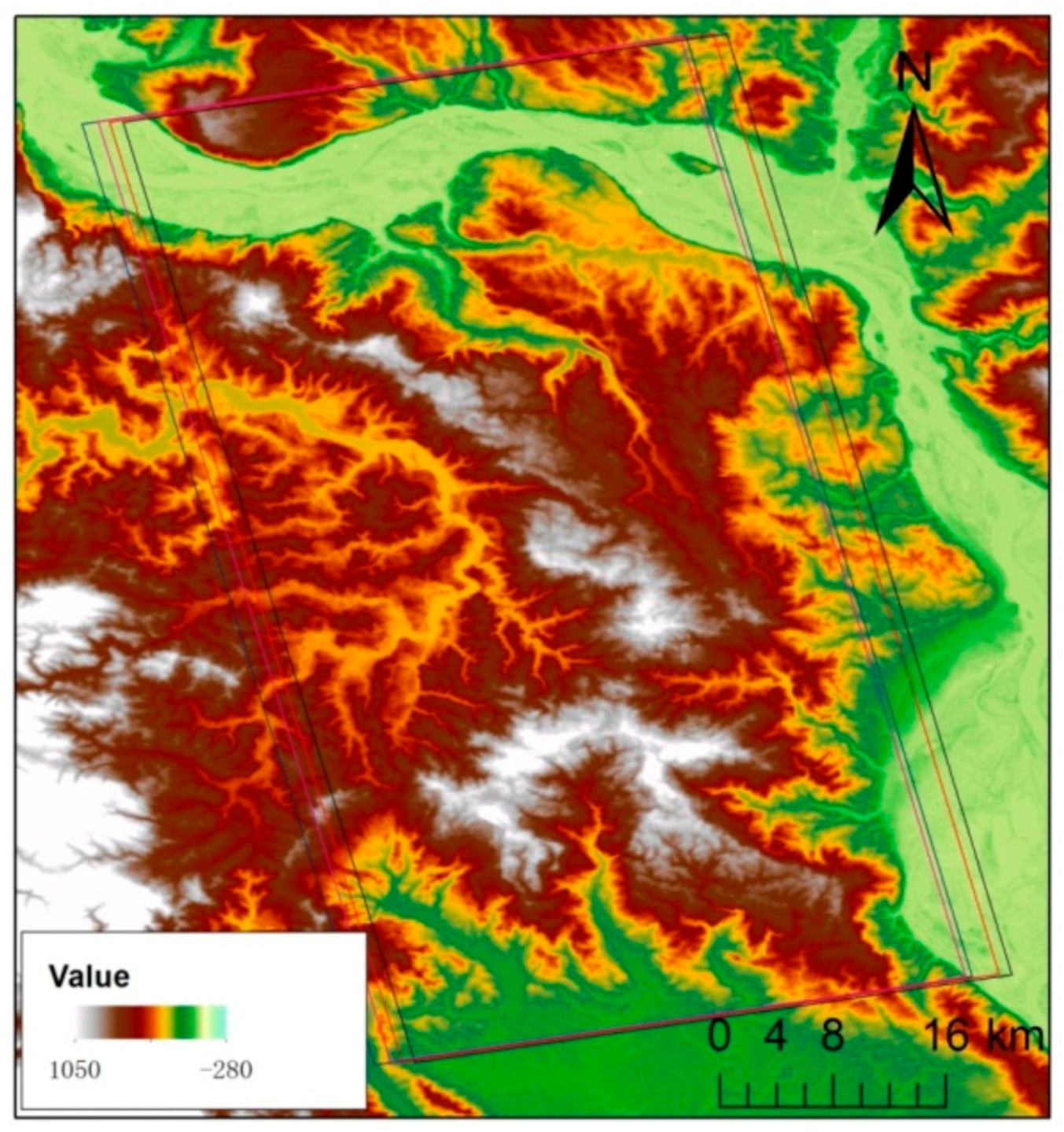
2.1. Study Area

The study area is located in Washington County and Columbia County, Oregon, on the west coast of the United States (Figure 1). Its forest coverage area is 1101.88 km², accounting for 47.8% of the total land area. The main forest types are coniferous forests with mixed distribution of evergreen coniferous forests and deciduous forests. The main tree species are Yellow fir, Sequoia sequoiae, Alnus koraiensis and California hemlock. The terrain is characterized by low mountains and hills with an elevation of 0–630 m and gentle slope (Figure 2). Forests are mainly located on slopes, of which 23.2% are located on the flat land with a slope of 0–5 degrees, 36% are located on gentle slopes of 5–10 degrees, and 2.6% are located on regions with a slope of higher than 24 degrees.

2.2. Data and Preprocessing

2.2.1. Remote-Sensing Data

The remote-sensing data used in this study include 4 full-polarized ALOS/PALSAR images and 2 Landsat/TM images. These data cover two counties of Columbia and Washington, OR, USA (Figure 3). The relevant information of the images was shown in

Table 1. The information of remote-sensing data used in this study.

No.	Dataset Name	Acquisition Date & Time	Format	SNR
73	PASL1100703160622521312040013	16 March 2007 06:22	DRSDAC-PLR L1.1	65.2
75	PASL1100705010622521312040015	1 May 2007 06:22	DRSDAC-PLR L1.1	38.2
93	PASL1100903210623171312040014	21 March 2009 06:23	DRSDAC-PLR L1.1	91.8
95	PASL1100905060623391312040016	6 May 2009 06:23	DRSDAC-PLR L1.1	185.3
TM73	LT50460282007088PAC01	29 March 2007 10:50	TIF	--
TM75	LT50460282007152PAC01	1 June 2007 10:50	TIF	--

. The spatial interference (e.g., baseline distance) of the four ALOS/PALSAR images paired separately was shown in

Table 2. The list of baselines of four ALOS/PALSAR image pairs

PolInSAR Image Pair	Spatial Baseline Distance (m)	Top Baseline Distance (m)	H2pi (m)	Temporal Baseline Distance (Days)	Kz
73–75	593.71	3727.91	61.22	46	0.103
75–95	1706.35	3727.91	21.31	736	0.295
73–93	1311.49	3727.91	27.72	736	0.227
93–95	198.91	3727.91	185.69	46	0.034

. As shown in Table 2, the maximum tree heights extracted from 73–93 and 75–95 InSAR image pairs are 27.72 m and 21.31 m, respectively. Since the maximum height of forest in the study area is 60.4 m, the estimation requirements cannot be satisfied. Therefore, this study mainly focused on the estimation and analysis using 73–75 and 93–95 InSAR image pairs.

Two simultaneous Landsat TM images were also collected for studies of time decoherence. The specific information was shown in Table 1. The SRTM DEM data covering the PALSAR data range (Figure 2) were collected to optimize the canopy height estimation algorithm.

2.2.2. Field Survey Data

The ground data used in this study was the ground survey results of 1999–2012 downloaded from the Forest Service Bureau of the United States Department of Agriculture. There were 121 ground points. The distribution of these ground points was shown in Figure 1. The accuracy of tree height measurement is ±0.5 m and the accuracy of ground positioning is ±0.8 m.

2.2.3. ALOS/PALSAR Data Pre-Processing

(a) Registration of the Main and the Secondary Images

PolInSAR technology extracts the phase from single-look complex (SLC) data files for canopy height estimation. Before the estimation based on PolInSAR, radiation and polarization calibration of SLC data with HH, HV and VV polarizations were needed, and then registration of two full-polarized SAR images acquired at a certain distance (main and secondary images) was conducted. Figure 4 is the interferometric phase diagram of 73–75 image pair in HV polarization, and Figure 5 is that of 93–95 image pair in HV polarization. Figure 4a and Figure 5a indicated that when the two SAR images were directly interfered, many fringes were obtained, including flat phase, terrain phase and canopy phase. In order to obtain canopy information, the flat and terrain phases should be removed. After the calibration and registration, the quality of the two SAR images was effectively improved (Figure 4b and Figure 5b).

(b) Removal of Terrain Phase from Secondary Images

Through the analysis of interferometric information, it was found that the flat and terrain phase should be removed to obtain canopy information. The vertical component of the baseline distance will lead to interferometric phase difference at different incident angles, and the equation is as follows.

$$f_s=\frac{2B_n}{\lambda R_{0}tan\theta }$$

(1)

Here, $f_s$ is the phase change rate under flat ground condition; R₀ is the slope distance; B_n is the vertical baseline distance; λ is the wavelength.

The terrain phase in the interferometric image needs to be removed based on DEM and observed geometric parameters. Assuming that the change rate of terrain phase is $f_{DEM}$, the flat and terrain phase can be eliminated by multiplying a complex conjugate phase on the basis of the original interference, as shown in Equation (2).

$$s_1{s}_2{e}^{-i2\pi \left(f_s+f_{DEM}\right)R_0}$$

(2)

Here, $s_1$ and $s_2$ represent the main image and the secondary image respectively. After removing the flat and terrain phase, only the canopy information is reserved. Before estimation of canopy height, the conversion factor between phase and height is also needed, which is the vertical wave-number.

(c) Estimation of Vertical Wave-Number

The vertical wave-number $k_z$ represents the phase change corresponding to the vertical height change of 1 m. Its unit is rad/m. See Equation (3).

$$k_z=\frac{4\pi \Delta \theta }{\lambda sin\theta }\approx \frac{4\pi B_n}{\lambda Htan\theta }$$

(3)

Here $\Delta \theta$ denotes the difference of incident angle between two observations; $\theta$ denotes the incident angle; and $\lambda$ denotes the wavelength, $B_n$ denotes the vertical baseline distance. Equation (3) shows that the vertical wave-number is a function of the incident angle. For a fixed baseline distance, $k_z$ is larger at short distance and small incident angle, but smaller at long distance and large incident angle, as shown in Figure 6.

Phase deviation caused by vegetation is not simply equivalent to tree height, but usually smaller than true height. This is due to the influence of the extinction coefficient, forest structure and ground scattering. In dense forest area, SAR signal cannot reach the ground, thus there is in need of forest canopy height estimation algorithm.

(d) Computation of Coherence Coefficient

Coherence coefficient is not only an important indicator to evaluate the registration accuracy of the main and secondary images, but also a basic parameter for canopy height estimation, which directly affects the accuracy of tree height estimation. Equation (4) is used for calculating the coherence coefficient.

$$\gamma =\frac{{{\displaystyle \sum }}_{i=1}^L{s}_{1i}{s}_{2i}^{*}}{\sqrt{{{\displaystyle \sum }}_{i=1}^L{s}_{1i}{s}_{1i}^{*}}\sqrt{{{\displaystyle \sum }}_{i=1}^L{s}_{2i}{s}_{2i}^{*}}}$$

(4)

Here, $s_{1i}$ and $s_{2i}$ represent the pixel values of two single-look images (complex numbers). L denotes the number of pixels participating in the statistics.

To analyze the influence of statistical window size on the estimation accuracy of coherent phase and amplitude, the scattering data covering the sample region of (528, 2050; 1182, 2552) were selected from a woodland (Figure 7) and the coherence calculation was performed using windows size of 3, 7, 11, 15, 19 and 23, respectively. The results are shown in

Table 3. The mean and standard deviation (SD) of coherence amplitude and phase for different statistical window size in 73–75 (H: Horizontal; V: Vertical).

Polarization Mode	3	7	11	15	19	23
	mean_amplitude
HH	0.574	0.408	0.380	0.375	0.375	0.376
HV	0.563	0.383	0.339	0.323	0.319	0.318
VV	0.588	0.413	0.372	0.356	0.351	0.347
HH-VV	0.558	0.367	0.332	0.328	0.327	0.328
	mean_phase
HH	−0.095	−0.136	−0.210	−0.244	−0.262	−0.278
HV	−0.071	−0.153	−0.193	−0.176	−0.153	−0.140
VV	−0.152	−0.098	−0.086	−0.095	−0.117	−0.148
HH-VV	−0.051	−0.071	−0.059	−0.079	−0.101	−0.126
	SD_amplitude
HH	0.210	0.165	0.104	0.067	0.051	0.046
HV	0.204	0.143	0.109	0.097	0.088	0.079
VV	0.209	0.154	0.118	0.103	0.090	0.082
HH-VV	0.213	0.167	0.119	0.086	0.074	0.068
	SD_phase
HH	1.198	0.730	0.415	0.325	0.275	0.241
HV	1.271	0.803	0.550	0.387	0.283	0.237
VV	1.243	0.833	0.613	0.505	0.450	0.387
HH-VV	1.333	0.907	0.514	0.374	0.298	0.234

and

Table 4. The mean and SD of coherence amplitude and phase for different statistical window size in 93–95.

Polarization Mode	3	7	11	15	19	23
	mean_amplitude
HH	0.701	0.649	0.641	0.637	0.635	0.633
HV	0.720	0.666	0.658	0.653	0.649	0.646
VV	0.740	0.694	0.687	0.688	0.691	0.692
HH-VV	0.697	0.639	0.632	0.630	0.630	0.631
	mean_phase
HH	0.474	0.476	0.461	0.458	0.459	0.464
HV	0.470	0.474	0.485	0.492	0.495	0.498
VV	0.606	0.609	0.606	0.601	0.602	0.602
HH-VV	0.550	0.527	0.511	0.508	0.508	0.509
	SD_amplitude
HH	0.190	0.116	0.086	0.075	0.068	0.064
HV	0.186	0.118	0.075	0.057	0.046	0.041
VV	0.178	0.121	0.099	0.083	0.071	0.057
HH-VV	0.188	0.115	0.078	0.061	0.055	0.053
	SD_phase
HH	0.648	0.283	0.182	0.131	0.109	0.097
HV	0.629	0.274	0.181	0.139	0.116	0.100
VV	0.560	0.264	0.174	0.138	0.118	0.105
HH-VV	0.636	0.267	0.168	0.131	0.106	0.092

.

As can be seen from Table 3, when the statistical window size is 7, the estimation result of coherent amplitude is similar to that of a larger window, but the estimation accuracy of the coherent phase is very poor. Until the window size increases to 23, the standard deviation (SD) of coherence coefficient is less than 0.24, which will lead to a height error of 2.4 m. In Table 4, for 93–95 image pairs, the SD of coherence coefficient is less than 0.1 and the estimated height error is 2.95 m when the window size is 23.

In addition to calculating the complex coherence coefficients of HH, HV, VV, HH+VV, HV+VH and HH-VV from Pauli decomposition, the phase diversity (PD) polarization interference coherence method and the singular value decomposition (SVD) technique were used to optimize the complex coherence coefficients. After obtaining high-precision complex coherence coefficients, four algorithms were adopted for canopy height estimation, respectively.

3. Methodology

3.1. Differential Digital Elevation Model (DEM) Algorithm

The differential DEM algorithm calculates the phase difference of different polarizations, one of which represents the ground phase and the other represents the top of the tree crown. Then, dividing the phase difference by the vertical wave-number, the tree height can be obtained, as shown in Equation (5).

$$h_v=\frac{arg({\tilde{\gamma }}_{{\underset{¯}{w}}_V})-\widehat{\varphi }}{k_z}$$

(5)

Here, $\widehat{\varphi }$ indicates ground phase. ${\tilde{\gamma }}_{{\underset{¯}{w}}_V}$ is the phase of the top layer of vegetation, which is often approximated by the phase of HV polarization.

There are many methods for choosing the two phases. In this study, two combinations were used. First, HV polarization was used to represent tree-top phase and HH-VV polarization was used to represent ground phase. The second method used the PD coherence decomposition algorithm to extract the high phase and low phase channels. The high phase was used to represent the top of the canopy (PD_High) and the low phase was used to represent the ground phase (PD_Low).

3.2. Coherent Amplitude Algorithm

Coherent amplitude algorithm estimates forest height through coherent amplitude with only one volume scattering channel. The principle is to calculate the tree height corresponding to the coherent amplitude based on the attenuation model of random scatters. When extinction coefficient is 0, the relationship between coherent amplitude and tree height is a sinc function, as shown in Equation (6). When extinction coefficient is not 0, Equation (7) is used for estimation.

$$sinc=e^{i{k}_z{z}_0}{e}^{i{k}_v\frac{h_v}{2}}\frac{sin(\frac{k_z{h}_v}{2})}{\frac{k_z{h}_v}{2}}$$

(6)

$$\underset{h_v}{min}{L}_1=\Vert \left|{\tilde{\gamma }}_{{\underset{¯}{w}}_V}\right|-\left|\frac{p}{p_1}\frac{e^{p_1{h}_v}-1}{e^{p{h}_v}-1}\right|\Vert where\left\{\begin{array}{l}p=\frac{2\sigma }{cos\theta }\\ p_1=p+i{k}_z\end{array}\right.$$

(7)

Here,$\theta$ denotes the incident angle; $h_v$ is the canopy height; and ${\tilde{\gamma }}_{{\underset{¯}{w}}_V}$ represents the coherent amplitude of the w_v channel.

3.3. Coherent Phase-Amplitude Algorithm

The coherent phase-amplitude algorithm combines the advantages of the differential DEM algorithm and the coherent amplitude algorithm. It takes into account the extinction coefficient and the vertical structure and has less computational complexity. The algorithm requires two interferometric channels, one is the ground-dominated channel $w_s$ and the other is the volume scattering-dominated channel $w_v$. The forest canopy height can be expressed by Equation (8).

$$\begin{array}{l}{h}_v=\frac{arg\left({\tilde{\gamma }}_{w_v}\right)-\widehat{\varphi }}{k_z}+\epsilon \frac{2sin{c}^{-1}\left(\left|{\tilde{\gamma }}_{w_v}\right|\right)}{k_z}\\ where\\ \widehat{\varphi }=arg\left({\tilde{\gamma }}_{{\underset{¯}{w}}_V}-{\tilde{\gamma }}_{{\underset{¯}{w}}_s}\left(1-L_{{\underset{¯}{w}}_s}\right)\right)0\le L_{{\underset{¯}{w}}_s}\le 1\\ A{L}_{{\underset{¯}{w}}_s}^2+B{L}_{{\underset{¯}{w}}_s}+C=0\Rightarrow L_{{\underset{¯}{w}}_s}=\frac{-B-\sqrt{B^2-4AC}}{2A}\\ A={\left|{\tilde{\gamma }}_{{\underset{¯}{w}}_s}\right|}^2-1\\ B=2Re\left(\left({\tilde{\gamma }}_{{\overline{w}}_V}-{\tilde{\gamma }}_{{\underset{¯}{w}}_s}\right)\cdot {\tilde{\gamma }}_{{\underset{¯}{w}}_s}^{*}\right)\\ C={\left|{\tilde{\gamma }}_{{\underset{¯}{w}}_V}-{\tilde{\gamma }}_{{\underset{¯}{w}}_s}\right|}^2\end{array}$$

(8)

Here, ${\tilde{\gamma }}_{w_v}$ represents the complex coherence coefficient of the $w_v$ channel, $\widehat{\varphi }$ denotes the ground phase, $k_z$ is the vertical wave-number and ε is the weight coefficient. Equation (8) consists of two parts. The first part is the phase height, that is, the phase difference between the canopy and the ground. Unlike Equation (5), this algorithm does not require the phase center of volume scattering to be located at the top of the tree, and uses coherent amplitude to compensate the low estimation. In this study, sinc function was used as theoretical amplitude to estimate tree height. Therefore, only a one-dimensional look-up table with extinction coefficient of 0 was needed.

The weight coefficient ε is very crucial. When extinction coefficient is 0, it is 0.5. When extinction coefficient increases to the maximum, the value of ε is reduced to 0, and the phase center is the tree height position. For L-band estimation, the extinction coefficient is not more than 0.1 dB/m. The algorithm considers both the accuracy and the computational complexity, thus is an optimized canopy height estimation algorithm based on PolInSAR. In this study, the parameters of canopy height estimation based on this model were set as follows: ε = 0.4; the ground channel and the volume scattering channel were set through two options: (1) HH-VV and HV polarization; (2) surface scattering coherence coefficient ${\gamma }_{w_s}$ and volume scattering coherence coefficient ${\gamma }_{w_v}$ from PD polarization interference PD_High and PD_Low.

3.4. Three-Stage Random Volume over Ground Algorithm (RVoG_3)

Here the RVoG model assumes the following coherence function:

$$\gamma \left(w\right)=e^{j{\varphi }_0}[{\gamma }_{vo}+\frac{\mu \left(w\right)}{1+\mu \left(w\right)}\left(1-{\gamma }_{vo}\right)]$$

(9)

In the vegetation vertical direction, the structure function of the model decreases exponentially, and the effect of understory surface scattering is taken into account. $\mu \left(w\right)$ is the polarization-dependent terrain scattering ratio, ${\gamma }_{vo}$ is a “pure” volume decoherence without terrain phase. Equation (9) shows that in the complex plane, the complex interference coherence is distributed in a straight line. One of the intersections of the straight line and the unit circle is the ground point. The distance between the volume scattering coherence and the terrain phase point is the farthest. Based on this principle, Cloude and Papathanassiou [27] proposed a three-stage RVoG algorithm:

(1)

Line fitting by least square method. Linear fitting was performed on the complex plane and the intersection points between the straight line and the unit circle were calculated. Generally, there were two intersections.

(2)

Ground points determination. The ground points were judged by the coherence value farthest from HV polarization.

(3)

Vegetation height estimation. First, the complex coherence coefficient was multiplied by $e^{-i\varphi }$ to remove the phase of the ground point. Then, the forest height and attenuation coefficient were obtained from a look-up table.

4. Results

4.1. Canopy Height Estimation Results

The canopy height was retrieved from 73–75 image pair and 93–95 image pair based on a differential DEM algorithm, coherent amplitude algorithm, coherent phase-amplitude algorithm, and three-stage RVoG algorithm, respectively. The statistical information of the results were obtained and are shown in

Table 5. The error table of the estimation methods for 73–75 (DEM_dif: the differential DEM algorithm which uses HV and HH-VV polarization to represent the canopy-top phase and the ground phase; DEM_pd: the differential DEM algorithm which uses the PD_High and PD_Low as the canopy-top and ground phase; Coh: the coherent amplitude algorithm; RVoG_3: the three-stage RVoG estimation algorithm; PC: the coherent phase-amplitude algorithm which uses the HV and HH-VV polarization to represent the canopy-top and the ground phase; PC_pd: the coherent phase-amplitude algorithm which uses the PD_High and PD_Low to represent the canopy-top and the ground phase).

Influence Factor	Level	Indicator	DEM_dif	DEM_pd	Coh	RVoG_3	PC	PC_pd
Overall	Overall	R2	0.00	0.06	0.07	0.07	0.01	0.00
		RMSE	12.96	11.55	12.96	13.66	7.47	8.10
		Mean value	−0.13	2.98	45.55	46.45	22.30	27.11
		Absolute error	−22.00	−18.88	23.68	23.68	0.44	5.24
Range slope level	<−5	R2	0.10	0.42	0.61	0.61	0.00	0.09
		RMSE	13.59	12.53	12.90	12.90	7.62	7.64
		Mean value	1.01	3.71	44.91	44.91	21.49	26.60
		Absolute error	−22.98	−20.27	20.93	20.93	−2.50	2.62
	[−5, 5]	R2	0.05	0.00	0.02	0.00	0.01	0.01
		RMSE	12.11	10.81	14.46	9.15	7.92	8.62
		Mean value	0.21	3.00	45.34	32.25	23.50	27.31
		Absolute error	−24.91	−22.12	20.22	7.13	−1.62	2.19
	>5	R2	0.00	0.12	0.18	0.38	0.02	0.08
		RMSE	14.20	12.17	13.00	6.65	6.51	7.54
		Mean value	−1.97	2.22	46.61	31.28	20.73	27.22
		Absolute error	−25.64	−21.46	22.94	7.60	−2.94	3.54
Coherence coefficient	<0.5	R2	0.00	0.01	0.00	0.02	0.01	0.01
		RMSE	13.21	11.82	13.40	7.90	7.33	7.88
		Mean value	−0.16	2.74	46.12	32.07	22.15	27.20
		Absolute error	−30.42	−27.52	15.87	1.82	−8.11	−3.06
	>0.5	R2	0.01	0.50	0.67	0.58	0.09	0.34
		RMSE	6.92	5.55	14.65	8.69	8.14	8.70
		Mean value	1.56	6.92	37.99	25.67	24.42	24.91
		Absolute error	−9.92	−4.55	26.51	14.19	12.94	13.44

and

Table 6. The error table of the estimation methods for 93–95.

Influence Factor	Level	Indicator	DEM_dif	DEM_pd	Coh	PC	PC_pd
Overall	Overall	R2	0.04	0.04	0.00	0.00	0.00
		RMSE	12.36	11.02	49.33	29.05	42.25
		Mean value	1.27	30.75	113.83	67.39	98.00
		Absolute error	−16.75	12.72	95.81	49.37	79.98
Range slope level	<−5	R2	0.06	0.04	0.04	0.00	0.08
		RMSE	14.07	10.99	50.38	33.46	41.33
		Mean value	−0.30	31.27	114.81	75.87	92.11
		Absolute error	−18.88	12.69	96.23	57.29	73.53
	[−5, 5]	R2	0.00	0.05	0.01	0.00	0.01
		RMSE	11.26	12.32	49.81	28.50	43.94
		Mean value	0.80	30.83	112.76	65.89	100.74
		Absolute error	−15.37	14.66	96.59	49.72	84.57
	>5	R2	0.30	0.09	0.17	0.02	0.01
		RMSE	12.71	7.88	48.87	26.24	40.78
		Mean value	3.85	30.05	115.14	62.67	98.03
		Absolute error	−17.44	8.75	93.85	41.38	76.74
Coherence coefficient	<0.5	R2	0.30	0.16	−0.04	0.06	−0.05
		RMSE	12.52	9.93	51.81	29.48	42.55
		Mean value	1.93	26.88	119.06	69.23	99.56
		Absolute error	−15.89	9.05	101.23	51.41	81.73
	>0.5	R2	0.01	0.14	0.00	0.00	0.00
		RMSE	12.28	11.97	45.93	28.72	42.35
		Mean value	0.71	36.05	106.59	64.91	98.78
		Absolute error	−17.70	17.63	88.17	46.49	80.36

. In the two tables, DEM_dif denotes the differential DEM algorithm which uses HV and HH-VV polarization to represent the canopy-top phase and the ground phase, respectively; DEM_pd denotes the differential DEM algorithm which uses the PD_High and PD_Low as the canopy-top and ground phase; Coh represents the coherent amplitude algorithm; RVoG_3 indicates the three-stage RVoG estimation algorithm; PC denotes the coherent phase-amplitude algorithm which uses the HV and HH-VV polarization to represent the canopy-top and the ground phase, respectively; PC_pd denotes the coherent phase-amplitude algorithm which uses the PD_High and PD_Low to represent the canopy-top and the ground phase, respectively.

From Table 5, it was found that the absolute errors of DEM_dif and DEM_pd algorithm were both less than 0, and the DEM_pd algorithm can reduce the low estimation relatively. By contrast, the absolute errors of the Coh algorithm and RVoG_3 algorithm were 23.68 m, which were significantly higher than true value. The absolute error of PC algorithm was 0.44 m, with the highest accuracy. Coh algorithm and RVoG_3 algorithm performed the best in terms of the determination coefficient (R²), but the R² was still too low, and there was also a large overestimation phenomenon. Comparing the performance of the RVoG_3 algorithm on different range slope levels, it can be found that the R² of canopy height on the slope against sensor direction was the highest. This was due to the fact that the ground-volume scattering ratio in SAR signal on the slope against sensor direction was smaller than that in flat terrain and sensor-oriented slope, and the volume scattering played a dominant role. Comparing the accuracy of each algorithm under different coherence coefficients of HV polarization, it can be found that when the coherence coefficient was greater than 0.5, the estimation effect was generally better than that of a coherence coefficient less than 0.5. Coh and RVoG_3 algorithms achieved higher R², reaching 0.67 and 0.58, reflecting the influence of the coherence coefficient on the estimation accuracy of canopy height.

Through the above analysis, it can be clearly seen that coherent optimization can effectively separate the phase, thus improving the accuracy of canopy height estimation using differential DEM algorithm. In this study, coherent amplitude was generally small, among which estimation results based on 73–75 SAR image pair were more reasonable. The height obtained by the differential DEM algorithm was half of the measured tree height, while the calculation error from 93–95 was larger. The results of the RVoG_3 algorithm based on the 93–95 image pair were almost invalid (thus not shown in Table 6). On the one hand, it was caused by the time decoherence; on the other hand, it was caused by the short baseline distance of 93–95, which leaded to the increase of ambiguity in height, thus increasing the influence of phase error on canopy height. Therefore, the algorithm optimization described later will only be conducted for the 73–75 image pair.

4.2. Optimized Canopy Height Estimation Considering Decoherence

To detect the effect of decoherence on the canopy height estimation accuracy, here four types of decoherence were considered and their results were compared. Firstly, the signal-to-noise ratio (SNR) was found from the metadata of 73 and 75 images, and the noise decoherence was calculated using Equation (10). The result was 0.98.

$${\gamma }_{snr}=\frac{{\left|a\right|}^2}{{\left|a\right|}^2+{\left|n\right|}^2}=\frac{SNR}{1+SNR}$$

(10)

Here, $a$ and $n$ refer to the effective information and noise; $SNR$ is the signal-to-noise ratio and ${\gamma }_{snr}$ indicates the noise decoherence.

The pre-processing decoherence caused by registration error was 0.97 through the calculation using Equation (11).

$${\gamma }_{proc}=\frac{sin\pi {\delta }_{rg}}{\pi {\delta }_{rg}}\frac{sin\pi {\delta }_{az}}{\pi {\delta }_{az}}$$

(11)

Here, ${\delta }_{rg}$ and ${\delta }_{az}$ indicate the deviation in the range and azimuth direction, respectively, ${\gamma }_{proc}$ indicates the pre-processing decoherence.

The baseline distance decoherence was 0.81 calculated by Equation (12).

$${\gamma }_B=\frac{B_{n,crit}-B_n}{B_{n,crit}}=1-\frac{B_n}{B_{n,crit}}=1-\frac{c{B}_n}{W\lambda R_{0}tan(\theta -\eta )}$$

(12)

Here, $c$ represents the speed of light, $W$ and $\lambda$ means the signal bandwidth and wavelength, $\theta$ and $\eta$ is the incident angle and slope in range direction, $B_n$ is the vertical baseline distance, ${\gamma }_B$ indicates the baseline distance decoherence.

The combination of the above three decoherences was 0.77. These decoherence factors were related to the coherent amplitude, but not to the phase, so dividing the coherence coefficients of the original image pair by 0.77, the coherence coefficient after decoherence were obtained. Finally, the canopy height was inverted using the Coh algorithm and RVoG_3 algorithm, as shown in

Table 7. The accuracy statistics of the results from Coh and RVoG_3 algorithms considering noise decoherence, pre-processing decoherence, and baseline distance decoherence.

Coherence Coefficient	Indicator	Coh	RVoG_3	Range Slope Level	Indicator	Coh	RVoG_3
Overall	R2	0.08	0.02	<−5	R2	0.54	0.49
	RMSE	11.93	8.02		RMSE	11.37	7.78
	Mean value	42.62	30.28		Mean value	41.80	29.54
	Absolute error	17.20	4.86		Absolute error	14.78	2.53
<0.5	R2	0.00	0.00	[−5, 5]	R2	0.00	0.01
	RMSE	11.80	7.85		RMSE	12.84	9.18
	Mean value	44.13	30.47		Mean value	42.87	30.94
	Absolute error	17.78	4.12		Absolute error	18.39	6.46
>0.5	R2	0.60	0.60	>5	R2	0.10	0.03
	RMSE	8.83	6.42		RMSE	10.89	5.65
	Mean value	34.91	28.21		Mean value	42.97	29.70
	Absolute error	12.81	6.12		Absolute error	17.27	4.00

.

Comparing Table 5 and Table 7, it was found that the overestimation of tree height by the Coh algorithm still existed, but it was suppressed after pre-processing decoherence, baseline distance decoherence and noise decoherence. The determination coefficient changed little, RMSE decreased from 12.96 m to 11.93 m, and absolute error decreased from 23.68 m to 17.20 m. The accuracy of the RVoG_3 algorithm was improved obviously when the coherence coefficient was greater than 0.5. The determination coefficient increased from 0.58 to 0.60, and absolute error decreased from 14.19 m to 6.12 m. This demonstrated the importance of decoherence processing for the forest parameter estimation algorithm. By comparing the estimation results of different coherence coefficients, it was found that the sample with higher coherence coefficients achieved higher estimation accuracy. This indicated that high coherence was an important guarantee for canopy height estimation with high precision.

Compared to the above three types of decoherence, time decoherence poses a difficulty for repeated observation technology. Considering PALSAR data were acquired in March and May, respectively, which was the season of vegetation growth in Oregon, the change of vegetation is the main factor leading to time decoherence. Thus, we used the NDVI variation from two Landsat/TM images acquired at the same date of PALSAR data to calculate the time decoherence. Then the total decoherence was obtained by the combination of noise decoherence, pre-processing decoherence, baseline distance decoherence and time decoherence. Considering the total decoherence, the canopy height was estimated by the RVoG_3 algorithm. Time decoherence was calculated by Equation (13).

$${\gamma }_t=1-2\frac{NDV{I}_5-NDV{I}_3}{NDV{I}_3+NDV{I}_5}$$

(13)

Here, NDVI₅ and NDVI₃ represent the NDVI values from TM images corresponding to the acquisition date of 75 and 73 PALSAR images, respectively.

Figure 8 is a scatter plot of the retrieved and measured canopy heights based on the RVoG_3 algorithm after time decoherence. It can be seen from the figure that although the R² was 0.2439, higher than the estimation result without time decoherence, the estimation result still had the problem of serious overestimation.

4.3. Optimized RVoG_3 Algorithm Considering Terrain

A previous study showed that the slope in azimuth direction had little influence on tree height, which can be ignored. Range slope was the main factor affecting canopy height estimation. In this study, the slope in range direction was extracted from SRTM-DEM, as shown in Figure 9, and canopy height estimation using the s-RVoG model was performed. Figure 10 shows the scatter plot of the canopy height estimation result from s-RVoG model and the field measured canopy height. As shown, the estimation considering time decoherence and terrain effect gave higher accuracy. Compared with Figure 8, it was found that the s-RVoG model performed better than the RVoG model. The R² was increased from 0.2439 to 0.3344, and the RMSE was reduced to 6.23 m.

5. Discussion

In this study, two InSAR image pairs, 73–75 and 93–95, were selected for estimation and analysis in the experimental areas of Washington and Columbia counties in the United States. It should be noted that the climate conditions during the acquisition date of the images have a great influence on the coherence coefficient of PolInSAR. According to the date and time of SAR image acquisition, the meteorological information of Portland, Longvilon, Astoria and Hillsborough stations around the study area was collected. Through comparative analysis, it was found that the meteorological conditions of 73 and 75 images were extremely similar, thus they had little influence on the coherence coefficient and the estimation accuracy; for the 93–95 image pair, it was foggy in Astoria station when acquiring the 93 image, and cloudy and rainy during the 95 image acquisition time, and thus visibility was quite low. Table 6 showed that canopy height was significantly overestimated on the 93–95 image pair based on a coherent amplitude algorithm. This was because when the data were acquired, the weather varied greatly, and thus the decoherence was large. From Table 3, it can be seen that the coherent amplitude of the vegetation area was only 0.35. These inevitably affected the coherence coefficient, which was one of the causes for the low precision of parameter estimation based on the 93–95 image pair in this study.

When calculating the coherence coefficient and exploring the influence of different window size on the estimation accuracy of coherent phase and coherent amplitude, the phase of the HV channel is usually higher than that of the HH-VV channel. But it can be seen from Table 3 and Table 4 that the interferometric phase of HV was lower than that of HH-VV channel. This phenomenon also exists in some simulated data, which has a certain impact on the accuracy of canopy height estimation, and the specific impact degree needs to be further studied.

In this study, when the differential DEM algorithm and the coherent phase-amplitude algorithm were applied, the phase difference of two different polarizations was necessary. Here two methods were used for choosing these two phases. First, HV polarization was used to represent tree-top phase and HH-VV polarization was used to represent ground phase. This assumption was used in areas where scattering is relatively small and the higher phase is HV. The phase height of HV polarization is between 1/2-1 of the canopy height, and is related to vegetation attributes such as extinction coefficient and canopy vertical structure. If the crown is higher and thinner, and the extinction coefficient is lower, the position of phase center is higher. On the other hand, when the crown is distributed in the whole vertical section, if the density is low, the height of the phase center is half of the tree height; if the density is high, the height of the phase center is equal to the tree height. The phase center of the dihedral scattering corresponds to the ground phase, thus as long as the dihedral scattering is stronger than the volume scattering, the ground phase can be approximated by this channel, while the HH-VV channel corresponds to the dihedral scattering component. Therefore, the two polarization phases were selected to estimate canopy height. This method had two shortcomings: (1) it seriously underestimated the tree height. This was because all polarization channels contained volume scattering information, and the phase center of volume scattering corresponded not to the tree-top, but to half the canopy height; (2) some of the canopy height estimation results were negative, as shown in Table 3 and Table 4. This was because the phase of HV became lower than that of HH-VV, which was contrary to the premise of this method.

The second method used the PD coherence decomposition algorithm. The high phase was used to represent the top of the canopy and the low phase was used to represent the ground phase. This decomposition algorithm was optimized for phase separation, which can maximize the separation of ground phase and canopy phase, and effectively improve the estimation accuracy. Their results were elaborately shown and compared in Table 5 and Table 6. Results indicated that PD coherence decomposition gave better performance than the HV polarization/HH-VV polarization assignment when the differential DEM algorithm was used. However, in the application of coherent phase-amplitude algorithm, opposite results were acquired although the difference between the two is not significant.

The problem of time decoherence is a key problem to be solved urgently in the PolInSAR system of repeated observation technology. It is also one of the main sources of PolInSAR parameter estimation error. In this study, Landsat/TM NDVI change rate is used to represent time decoherence to effectively improve the accuracy of canopy height estimation. The radiation transmission path and mechanism of visible and near infrared bands in vegetation canopy are quite different from those of L band. Meanwhile, the acquisition time of SAR data in this study is just the growing season of vegetation. The applicability of these algorithms in other sample areas and other time needs to be further studied.

RVoG model is one of the most successful PolInSAR models for forest vertical parameters estimation based on PolInSAR technology. The ground-volume scattering ratio is an important parameter of the model, which has a great influence on the accuracy of canopy height estimation. In this study, it is set as a constant. In order to improve the accuracy of canopy height estimation, the ground-volume scattering ratio estimation method will be taken into consideration aiming at different forest structure types. Additionally, the combination of RVoG model and other methodology (e.g., volume temporal decorrelation method in [45]) should be explored and compared.

Finally, as LiDAR has also been widely used for the forest canopy height estimation, and usually achieves high accuracy [12], the combination of LiDAR and SAR data to obtain forest canopy height will be meaningful and challenging work [16]. LiDAR and SAR are two main methods of active remote-sensing acquisition. Both of them can penetrate through the forest canopy to obtain the information of understory terrain and canopy vertical structure. However, there are obvious differences between the two remote-sensing technologies in data storage and parameter extraction. For example, LiDAR uses point cloud/waveform vector for storage and SAR uses raster for storage; and LiDAR mainly extracts parameters based on spatial distribution characteristics of point cloud, and SAR is mainly based on scattering matrix and backscattering coefficients. These characteristics also provide a good theoretical basis for the LiDAR and SAR combination to acquire canopy height. According to percentage of canopy point clouds in the total LiDAR point clouds, we have separated the ground points and vegetation canopy to obtain DEM and forest coverage; according to the Beer–Lambert law, the canopy extinction coefficient was inversed; based on the Beer–Lambert law and the vertical distribution of point clouds, the vertical profile of the canopy was obtained. Considering that DEM extinction coefficient and canopy vertical profile correspond to the terrain, extinction coefficient and vertical changes of the extinction coefficient in the RVoG model, the three parameters will be respectively brought into RVoG model to conduct canopy height estimation. The estimation accuracy is expected to achieve a significant improvement in combination of LiDAR and PolInSAR technology.

6. Conclusions

This study explored the forest canopy height estimation algorithm based on PolInSAR technology and analyzed its accuracy. Two PolInSAR image pairs were constructed based on four full-polarized ALOS/PALSAR images. The four methods of differential DEM algorithm, coherent amplitude algorithm, coherent phase-amplitude algorithm and a three-stage RVoG algorithm were used to estimate forest canopy height, and the accuracy was verified using field measured canopy height data. The results showed that the canopy height estimated by the differential DEM algorithm was seriously underestimated, while the coherent amplitude algorithm and the RVoG_3 algorithm overestimated the height. By removing the system coherence, the overestimation of the RVoG_3 model was suppressed, and the absolute error was reduced from 23.68 m to 4.86 m. After the time decoherence using the NDVI change rate of two Landsat/TM images, the determination coefficient was increased. By comparing the estimation results of different coherence coefficients, it was found that the estimation accuracy of canopy height was relatively higher at the sample points with higher coherence coefficients. By introducing the slope in the range direction from SRTM-DEM, the accuracy of canopy height estimation using the s-RVoG model was also improved significantly compared with using the RVoG model, which showed that the determination coefficient was increased from 0.2439 to 0.3344. This conclusion will provide a reference for algorithm selection when using ALOS/PALSAR data for forest canopy height estimation.

References

1. Stenseth, N.C. Ecosystem dynamics of the boreal forest: The Kluane project. Nature 2002, 416, 679–680. [Google Scholar] [CrossRef]
2. Chen, W.; Jiang, H.Z.; Moriya, K.; Sakai, T.; Cao, C.X. Monitoring of post-fire forest regeneration under different restoration treatments based on ALOS/PALSAR data. New For. 2018, 49, 105–121. [Google Scholar] [CrossRef]
3. Morford, S.L.; Houlton, B.Z.; Dahlgren, R.A. Increased forest ecosystem carbon and nitrogen storage from nitrogen rich bedrock. Nature 2011, 477, 78–88. [Google Scholar] [CrossRef] [PubMed]
4. Chen, W.; Zhao, J.; Cao, C.X.; Tian, H.J. Shrub biomass estimation in semi-arid sandland ecosystem based on remote sensing technology. Glob. Ecol. Conserv. 2018, 16, e00479. [Google Scholar] [CrossRef]
5. Izzawati, I.H.W.; Wallington, E.D.; Woodhouse, I.H. Forest height retrieval from commercial X-band SAR products. IEEE Trans. Geosci. Remote Sens. 2006, 44, 863–870. [Google Scholar] [CrossRef]
6. Laurin, G.V.; Ding, J.; Disney, M.; Bartholomeus, H.; Valentini, R. Tree height in tropical forest as measured by different ground, proximal, and remote sensing instruments, and impacts on above ground biomass estimates. Int. J. Appl. Earth Obs. Geoinf. 2019, 82, 101899. [Google Scholar] [CrossRef]
7. Liao, Z.; He, B.B.; Quan, X.; Van Dijk, A.I.J.M.; Qiu, S.; Yin, C. Biomass estimation in dense tropical forest using multiple information from single-baseline P-band PolInSAR data. Remote Sens. Environ. 2019, 221, 489–507. [Google Scholar] [CrossRef]
8. Liang, S.L. Quantitative Remote Sensing of Land Surfaces; John Wiley & Sons, Inc.: Hoboken, NJ, USA, 2004. [Google Scholar]
9. Ghulam, A.; Porton, I.; Freeman, K. Detecting subcanopy invasive plant species in tropical rainforest by integrating optical and microwave (InSAR/PolInSAR) remote sensing data, and a decision tree algorithm. ISPRS J. Photogramm. Remote Sens. 2014, 88, 174–192. [Google Scholar] [CrossRef]
10. Neeff, T.; Dutra, L.V.; dos Santos, J.R.; Freitas, C.D.; Araujo, L.S. Tropical forest stand table modeling from SAR data. For. Ecol. Manag. 2003, 186, 159–170. [Google Scholar] [CrossRef]
11. Chen, W.; Cao, C.X.; He, Q.S.; Guo, H.D.; Zhang, H.; Li, R.Q.; Zheng, S.; Xu, M.; Gao, M.X.; Zhao, J.; et al. Quantitative estimation of the shrub canopy LAI from atmosphere-corrected HJ-1 CCD data in Mu Us Sandland. Sci. China Earth Sci. 2010, 53, 26–33. [Google Scholar] [CrossRef] [Green Version]
12. Edson, C.; Wing, M.G. Airborne Light Detection and Ranging (LiDAR) for Individual Tree Stem Location, Height, and Biomass Measurements. Remote Sens. 2011, 3, 2494–2528. [Google Scholar] [CrossRef] [Green Version]
13. Cao, C.X.; Bao, Y.F.; Xu, M.; Chen, W.; Zhang, H.; He, Q.S.; Li, Z.Y.; Guo, H.D.; Li, J.H.; Li, X.W. Retrieval of forest canopy attributes based on Geometric-Optical model using airborne LiDAR and optical remote sensing data. Int. J. Remote Sens. 2012, 33, 692–709. [Google Scholar] [CrossRef]
14. Shimoni, M.; Borghys, D.; Heremans, R.; Perneel, C.; Acheroy, M. Fusion of PolSAR and PolInSAR data for land cover classification. Int. J. Appl. Earth Obs. Geoinf. 2009, 11, 169–180. [Google Scholar] [CrossRef]
15. Tahraoui, S.; Clemente, C.; Pallotta, L.; Soraghan, J.J.; Ouarzeddine, M. Covariance Symmetries Detection in PolInSAR Data. IEEE Trans. Geosci. Remote Sens. 2018, 56, 6927–6939. [Google Scholar] [CrossRef]
16. Brigot, G.; Simard, M.; Colin-Koeniguer, E.; Boulch, A. Retrieval of Forest Vertical Structure from PolInSAR Data by Machine Learning Using LIDAR-Derived Features. Remote Sens. 2019, 11, 381. [Google Scholar] [CrossRef] [Green Version]
17. Chen, L.; Wang, Y.Q.; Ren, C.Y.; Zhang, B.; Wang, Z.M. Assessment of multi-wavelength SAR and multispectral instrument data for forest aboveground biomass mapping using random forest Kriging. For. Ecol. Manag. 2019, 447, 12–25. [Google Scholar] [CrossRef]
18. Ghasemi, N.V.; Tolpekin, A.; Stein, A. Estimating Tree Heights Using Multibaseline PolInSAR Data With Compensation for Temporal Decorrelation, Case Study: AfriSAR Campaign Data. IEEE J. Sel. Top. Appl. Earth Obs. Remote Sens. 2018, 11, 3464–3477. [Google Scholar] [CrossRef]
19. Xie, J.W.; Suo, Z.Y.; Li, Z.F.; Wang, Y.K. High-precision Digital Surface Model Inversion Approach in Forest Region Based on PolInSAR. J. Elec. Inform. Tech. 2019, 41, 293–301. [Google Scholar]
20. Managhebi, T.; Maghsoudi, Y.M.; Zoej, J.V. A Volume Optimization Method to Improve the Three-Stage Inversion Algorithm for Forest Height Estimation Using PolInSAR Data. IEEE Geosci. Remote. Sens. Lett. 2018, 15, 1214–1218. [Google Scholar] [CrossRef]
21. Balzter, H.; Rowland, C.S.; Saich, P. Forest canopy height and carbon estimation at Monks Wood National Nature Reserve, UK, using dual-wavelength SAR interferometry. Remote Sens. Environ. 2007, 108, 224–239. [Google Scholar] [CrossRef]
22. Breidenbach, J.; Koch, B.; Kaendler, G.; Kleusberg, A. Quantifying the influence of slope, aspect, crown shape and stem density on the estimation of tree height at plot level using lidar and InSAR data. Int. J. Remote Sens. 2008, 29, 1511–1536. [Google Scholar] [CrossRef]
23. Arnaubec, A.; Roueff, A.; Dubois-Fernandez, P.C.; Refregier, P. Influence of the nature of a priori knowledge on the precision of vegetation height estimation in polarimetric SAR interferometry. In Proceedings of the European Conference on Synthetic Aperture Radar, Nuremberg, Germany, 23–26 April 2012; VDE: Berlin, Germany, 2012. [Google Scholar]
24. Cloude, S.R.; Papathanassiou, K.P. Polarimetric SAR interferometry. IEEE Trans. Geosci. Remote Sens. 1998, 36, 1551–1565. [Google Scholar] [CrossRef]
25. Yamada, H.; Yamaguchi, Y.; Rodriguez, E.; Kim, Y.; Boerner, W.M. Polarimetric SAR interferometry for forest analysis based on the ESPRIT algorithm. IEEE Trans. Electron. 2001, E84C, 1917–1924. [Google Scholar]
26. Lee, S.K.; Kugler, F.; Papathanassiou, K.; Hajnsek, I. Multibaseline polarimetric SAR interferometry forest height inversion approaches. In Proceedings of the 5th International Workshop on Science and Applications of SAR Polarimetry and Polarimetric Interferometry, Frascati, Italy, 24–28 January 2011; ESA: Frascati, Italy, 2011. [Google Scholar]
27. Cloude, S.R.; Papathanassiou, K.P. Three-stage inversion process for polarimetric SAR interferometry. IEE Proc. Radar Sonar Navig. 2003, 150, 125–134. [Google Scholar] [CrossRef] [Green Version]
28. Angiuli, E.; Del Frate, F.; Della Vecchia, A.; Lavalle, M.; Solimini, D.; Licciardi, G. Inversion algorithms comparison using L-band simulated polarimetric interferometric data for forest parameters estimation. In Proceedings of the 2007 IEEE International Geoscience and Remote Sensing Symposium (IGARSS), Barcelona, Spain, 23–28 July 2007. [Google Scholar]
29. Li, X.W.; Guo, H.D.; Liao, J.J. Retrieval of surface vegetation parameters based on spacecraft polarization interferometric radar data. J. Remote. Sens. 2002, 6, 424–429. [Google Scholar]
30. Yu, D.Y.; Dong, G.W.; Yang, J. Forest tree height inversion based on interferometric polarization SAR data. J. Tsinghua Univ. Nat. Sci. Ed. 2005, 3, 334–336. [Google Scholar]
31. Zhou, G.Y.; Xiong, T.; Zhang, W.J.; Yang, J. Tree height inversion method based on polarization interferometric SAR data. J. Tsinghua Univ. Nat. Sci. Ed. 2009, 4, 510–513. [Google Scholar]
32. Ghasemi, N.; Tolpekin, V.; Stein, A. A modified model for estimating tree height from PolInSAR with compensation for temporal decorrelation. Int. J. Appl. Earth Obs. Geoinf. 2018, 73, 313–322. [Google Scholar] [CrossRef]
33. Biondi, F. A new maximum likelihood polarimetric interferometric synthetic aperture radar coherence change detection (ML-PolInSAR-CCD). Int. J. Remote Sens. 2019, 40, 5158–5178. [Google Scholar] [CrossRef]
34. Treuhaft, R.N.; Madsen, S.N.; Moghaddam, M.; van Zyl, J.J. Vegetation characteristics and underlying topography from interferometric radar. Radio Sci. 1996, 31, 1449–1485. [Google Scholar] [CrossRef]
35. Treuhaft, R.N.; Siqueira, P.R. Vertical structure of vegetated land surfaces from interferometric and polarimetric radar. Radio Sci. 2000, 35, 141–177. [Google Scholar] [CrossRef] [Green Version]
36. Li, Z.; Guo, M.; Wang, Z.Q.; Zhao, L.F. Forest-height inversion using repeat-pass spaceborne polInSAR data. Sci. China Earth Sci. 2014, 57, 1314–1324. [Google Scholar] [CrossRef]
37. Ballester-Berman, J.D.; Vicente-Guijalba, F.; Lopez-Sanchez, J.M. A Simple RVoG Test for PolInSAR Data. IEEE J. Sel. Top. Appl. Earth Obs. Remote Sens. 2015, 8, 1028–1040. [Google Scholar] [CrossRef] [Green Version]
38. Sportouche, H.; Roueff, A.; Dubois-Fernandez, P.C. Precision of Vegetation Height Estimation Using the Dual-Baseline PolInSAR System and RVoG Model with Temporal Decorrelation. IEEE Trans. Geosci. Remote Sens. 2018, 56, 4126–4137. [Google Scholar] [CrossRef]
39. Praks, J.; Hallikamen, M.; Kugler, F.; Papathanassiou, K.P. X-band extinction in boreal forest: Estimation by using E-SAR POLInSAR and HUTSCAT. In Proceedings of the 2007 IEEE International Geoscience and Remote Sensing Symposium (IGARSS), Barcelona, Spain, 23–28 July 2007. [Google Scholar]
40. Garestier, F.; Toan, T.L. Forest modeling for height inversion using single-baseline InSAR/Pol-InSAR Data. IEEE Trans. Geosci. Remote Sens. 2010, 48, 1528–1539. [Google Scholar] [CrossRef]
41. Neumann, M.; Ferro-Famil, L.; Reigber, A. Estimation of Forest Structure, Ground, and Canopy Layer Characteristics from Multibaseline Polarimetric Interferometric SAR Data. IEEE Trans. Geosci. Remote Sens. 2010, 48, 1086–1104. [Google Scholar] [CrossRef] [Green Version]
42. Roueff, A.; Arnaubec, A.; Dubois-Fernandez, P.C.; Refregier, P. Cramer–Rao Lower Bound Analysis of Vegetation Height Estimation With Random Volume Over Ground Model and Polarimetric SAR Interferometry. IEEE Geosci. Remote Sens. Lett. 2011, 8, 1115–1119. [Google Scholar] [CrossRef]
43. Feng, Q.; Zhou, L.; Chen, E.; Liang, X.; Zhao, L.; Zhou, Y. The Performance of Airborne C-Band PolInSAR Data on Forest Growth Stage Types Classification. Remote Sens. 2017, 9, 955. [Google Scholar] [CrossRef] [Green Version]
44. Khati, U.; Singh, G.; Kumar, S. Potential of Space-Borne PolInSAR for Forest Canopy Height Estimation Over India-A Case Study Using Fully Polarimetric L-, C-, and X-Band SAR Data. IEEE J. Sel. Top Appl. Earth Obs. Remote Sens. 2018, 11, 2406–2416. [Google Scholar] [CrossRef]
45. Managhebi, T.; Maghsoudi, Y.; Valadan Zoej, M.J. Four-Stage Inversion Algorithm for Forest Height Estimation Using Repeat Pass Polarimetric SAR Interferometry Data. Remote Sens. 2018, 10, 1174. [Google Scholar] [CrossRef] [Green Version]
Figure 1. The spatial distribution of the field sample plots and remote-sensing data.
Remotesensing 13 00174 g001
Figure 2. The digital elevation model (DEM) map of the study area.
Remotesensing 13 00174 g002
Figure 3. The Pauli decomposition of the four Advanced Land Observing Satellite/Phased Array type L-band Synthetic Aperture Radar (ALOS/PALSAR) data.
Remotesensing 13 00174 g003
Figure 4. The interferometric phase diagram of the 73–75 image pair in HV (Horizontal-Vertical) polarization. (a) Before removal of terrain phase; (b) After removal of terrain phase
Remotesensing 13 00174 g004
Figure 5. The interferometric phase diagram of the 93–95 image pair in HV polarization. (a) Before removal of terrain phase; (b) After removal of terrain phase
Remotesensing 13 00174 g005
Figure 6. The gradient map of kz in range orientation: (a) 73–75; (b) 93–95 (X: distance; Y: kz).
Remotesensing 13 00174 g006
Figure 7. The CHM (canopy height model) and DEM of the statistical sample area. (a) CHM; (b) DEM.
Remotesensing 13 00174 g007
Figure 8. The scatter plot of field forest canopy height and those from RVoG_3 algorithm considering noise decoherence, pre-processing decoherence, baseline distance decoherence and time decoherence.
Remotesensing 13 00174 g008
Figure 9. The slope map of the study area in the range direction.
Remotesensing 13 00174 g009
Figure 10. The scatter plots of s-RVoG estimation result considering all four decoherence and terrain effects.
Remotesensing 13 00174 g010