Investigating Ground Subsidence and the Causes over the Whole Jiangsu Province, China Using Sentinel-1 SAR Data


Abstract
:1. Introduction
2. Materials and Methods
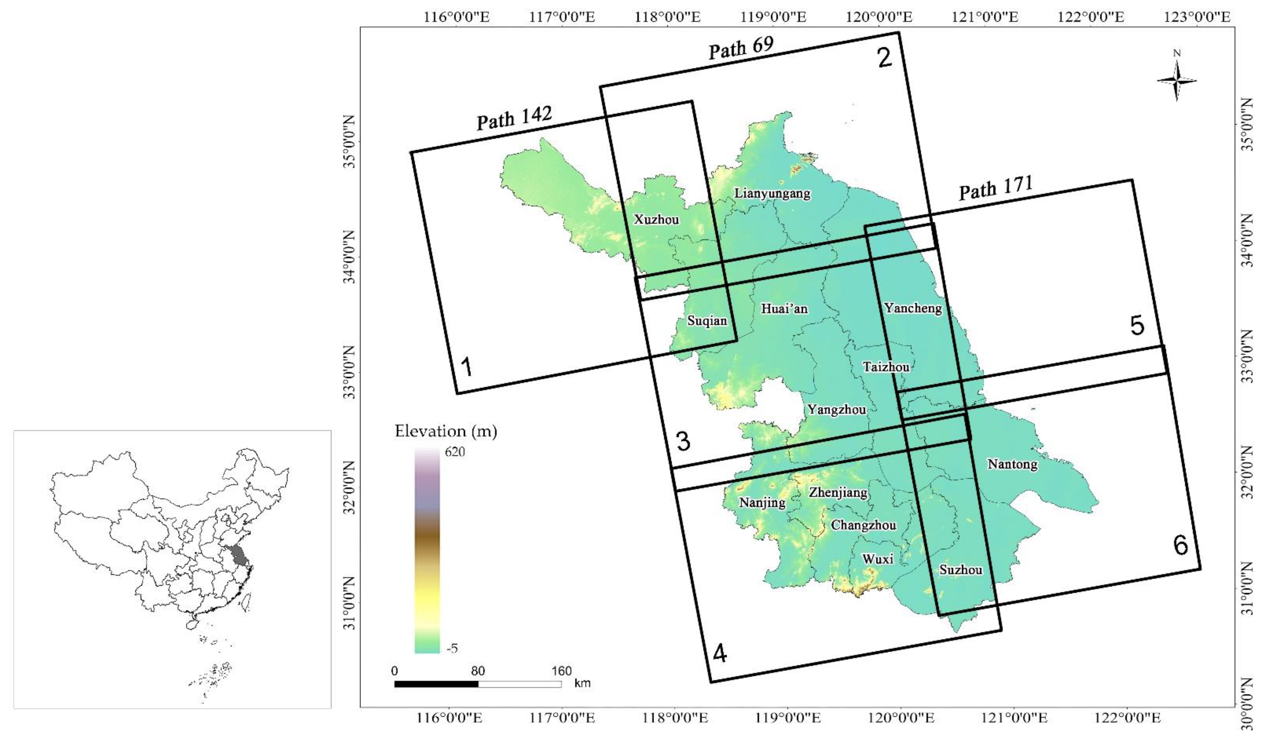
2.1. S-1 Data and the Study Area
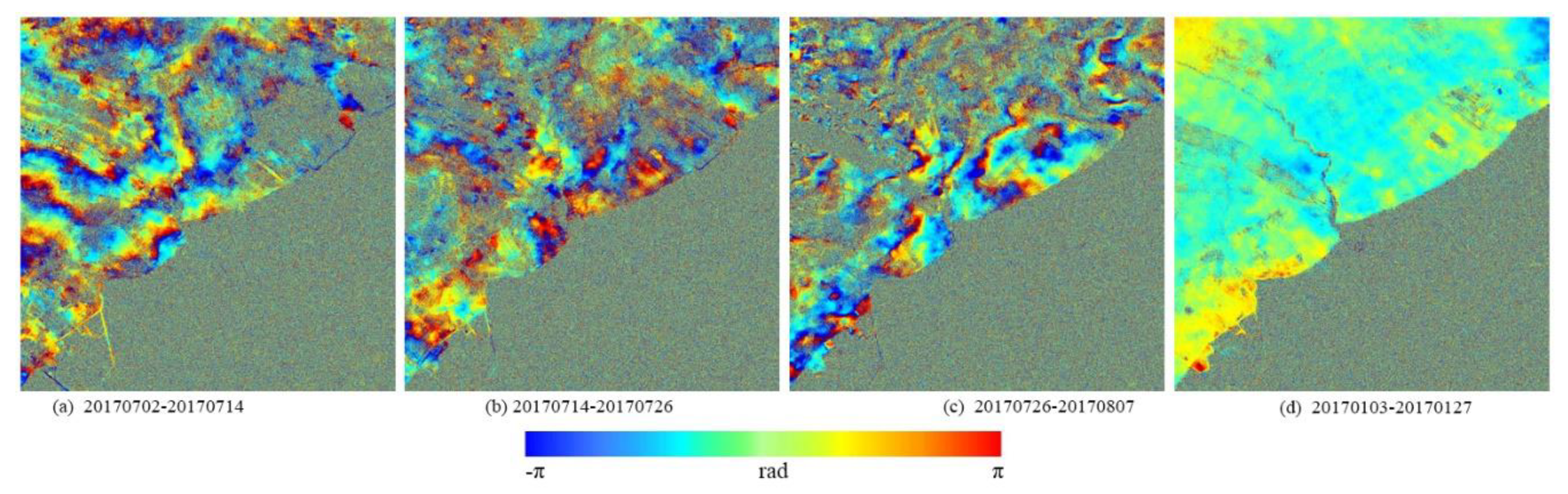
2.2. Data Processing
3. Results
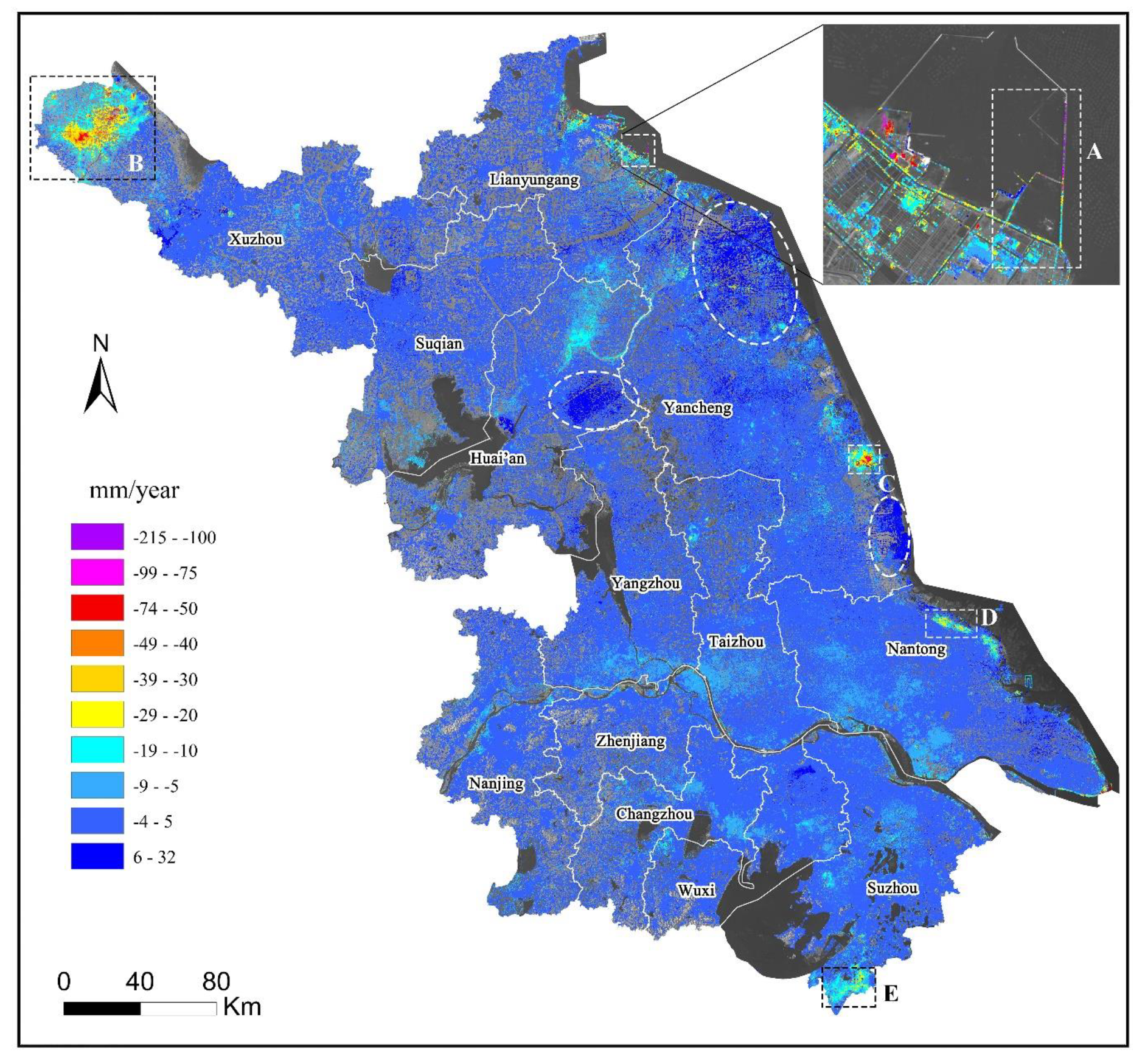
3.1. InSAR Results
3.2. Accuracy Evaluation
4. Discussion
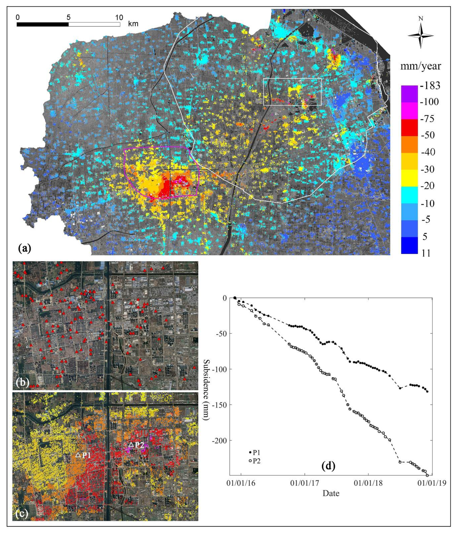
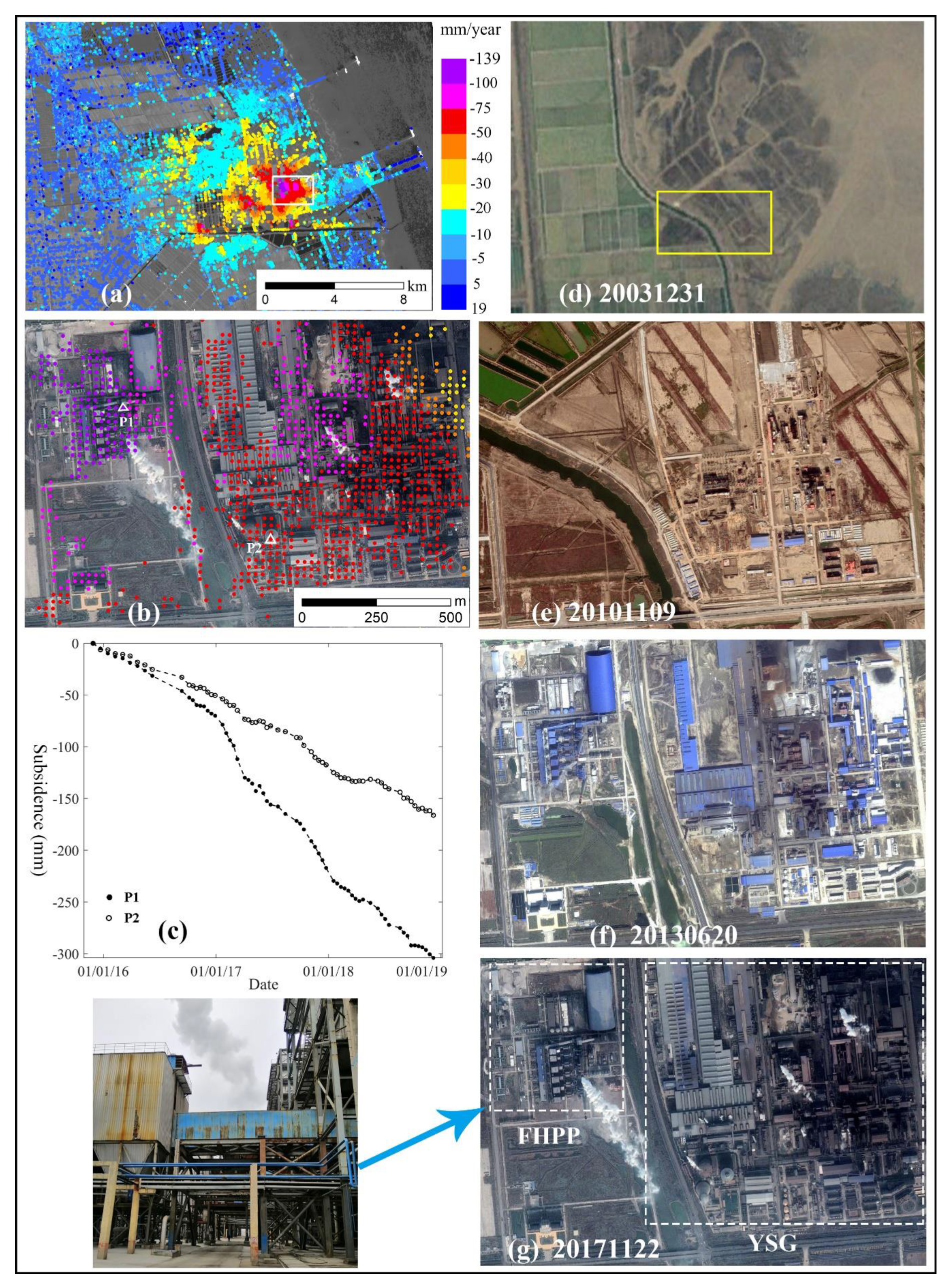
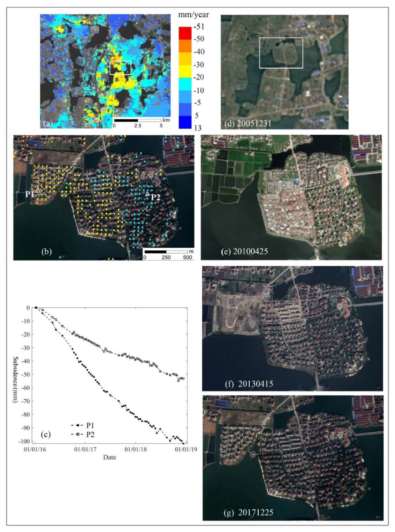
4.1. Subsidence Zone A
4.2. Subsidence Zone B
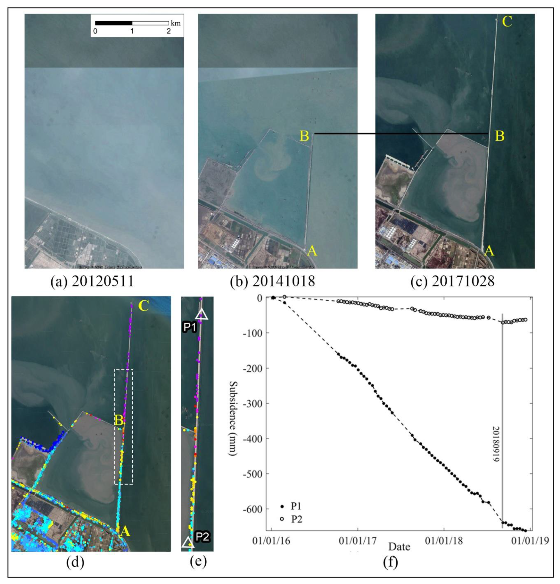
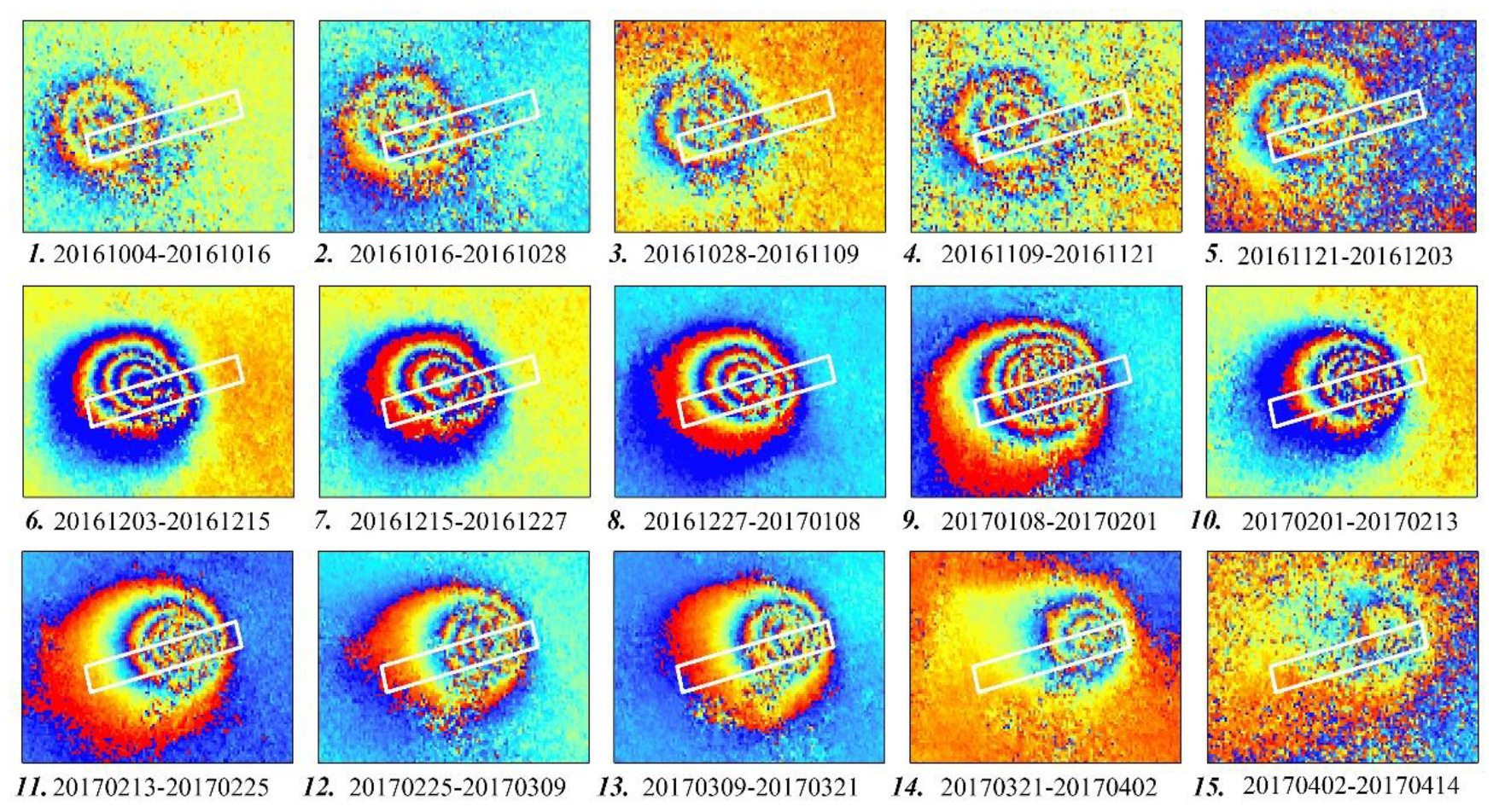
4.3. Subsidence Zone C
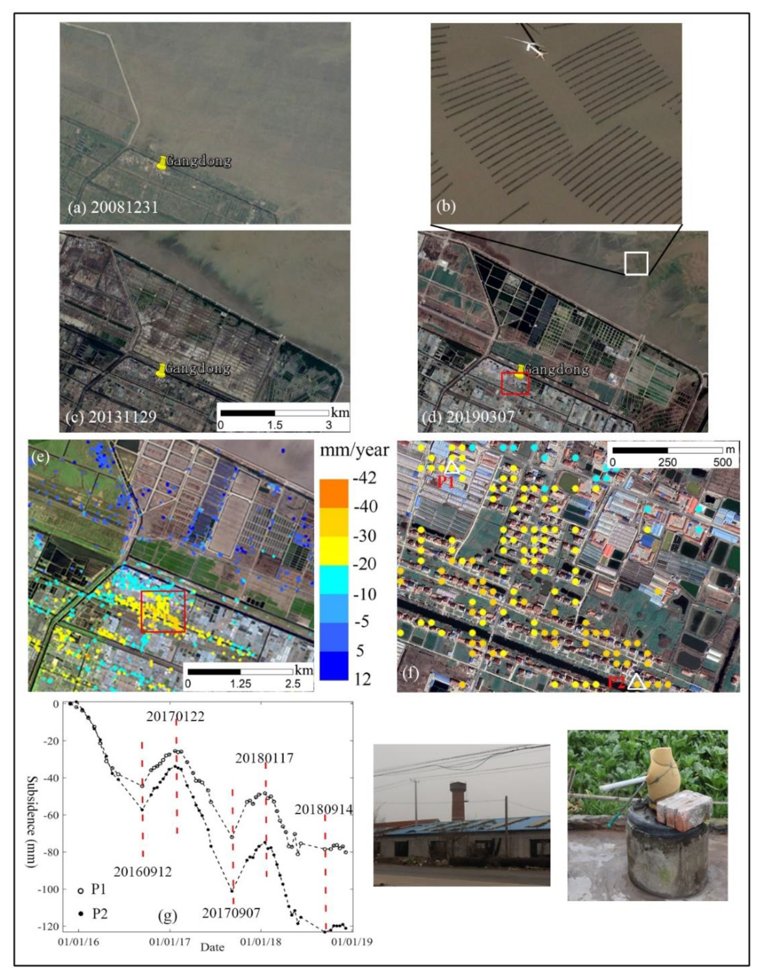
4.4. Subsidence Zone D
4.5. Subsidence Zone E
4.6. Comparative Analysis of Three Subsidence Scenarios
5. Conclusions
Author Contributions
Funding
Institutional Review Board Statement
Informed Consent Statement
Data Availability Statement
Acknowledgments
Conflicts of Interest
References
- Jiang, H. Problems and discussions in the study of land subsidence in the Suzhou-Wuxi-Changzhou area. Quat. Sci. 2005, 25, 29–33. [Google Scholar]
- Ferretti, A.; Prati, C.; Rocca, F. Nonlinear subsidence rate estimation using permanent scatterers in differential SAR interferometry. IEEE Trans. Geosci. Remote Sens. 2000, 38, 2202–2212. [Google Scholar] [CrossRef] [Green Version]
- Ferretti, A.; Prati, C.; Rocca, F. Permanent scatterers in SAR interferometry. IEEE Trans. Geosci. Remote Sens. 2001, 39, 8–20. [Google Scholar] [CrossRef]
- Berardino, P.; Fornaro, G.; Lanari, R.; Sansosti, E. A new algorithm for surface deformation monitoring based on small baseline differential interferograms. IEEE Trans. Geosci. Remote Sens. 2002, 40, 2375–2383. [Google Scholar] [CrossRef] [Green Version]
- Adam, N.; Parizzi, A.; Eineder, M.; Crosetto, M. Practical persistent scatterer processing validation in the course of the Terrafirma project. J. Appl. Geophys. 2009, 69, 59–65. [Google Scholar] [CrossRef] [Green Version]
- Zhang, L.; Lu, Z.; Ding, X.; Jung, H.; Feng, G.; Lee, C.W. Mapping ground surface deformation using temporarily coherent point SAR interferometry: Application to Los Angeles Basin. Remote Sens. Environ. 2012, 117, 429–439. [Google Scholar] [CrossRef]
- Qu, F.; Lu, Z.; Zhang, Q.; Bawden, G.W.; Kim, J.W.; Zhao, C.; Qu, W. Mapping ground deformation over Houston-Galveston, Texas using multi-temporal InSAR. Remote Sens. Environ. 2015, 169, 290–306. [Google Scholar] [CrossRef]
- Chen, M.; Tomás, R.; Li, Z.; Motagh, M.; Li, T.; Hu, L.; Gong, H.; Li, X.; Yu, J.; Gong, X. Imaging land subsidence induced by groundwater extraction in Beijing (China) using satellite radar interferometry. Remote Sens. 2016, 8, 468. [Google Scholar] [CrossRef] [Green Version]
- Zhou, C.; Gong, H.; Zhang, Y.; Warner, T.A.; Wang, C. Spatiotemporal evolution of land subsidence in the Beijing Plain 2003–2015 using Persistent Scatterer Interferometry (PSI) with multi-source SAR data. Remote Sens. 2018, 10, 552. [Google Scholar] [CrossRef] [Green Version]
- Luo, Q.; Perissin, D.; Lin, H.; Zhang, Y.; Wang, W. Subsidence monitoring of Tianjin suburbs by TerraSAR-X persistent scatterers interferometry. IEEE J. Sel. Top. Appl. Earth Observ. Remote Sens. 2014, 7, 1642–1650. [Google Scholar]
- Liu, G.; Luo, X.; Chen, Q.; Huang, D.; Ding, X. Detecting Land Subsidence in Shanghai by PS-Networking SAR Interferometry. Sensors 2008, 8, 4725–4741. [Google Scholar] [CrossRef] [PubMed] [Green Version]
- Zhang, Y.; Zhang, J.; Wu, H.; Lu, Z.; Sun, G. Monitoring of urban subsidence with SAR interferometric point target analysis: A case study in Suzhou, China. Int. J. Appl. Earth Observ. Geoinform. 2011, 13, 812–818. [Google Scholar] [CrossRef]
- Costantini, M.; Ferretti, A.; Minati, F.; Falco, S.; Trillo, F.; Colombo, D.; Novali, F.; Malvarosa, F.; Mammone, C.; Vecchioli, F.; et al. Analysis of surface deformations over the whole Italian territory by interferometric processing of ERS, Envisat and COSMO-SkyMed radar data. Remote Sens. Environ. 2017, 202, 250–275. [Google Scholar] [CrossRef]
- Zhang, Y.; Wu, H.; Kang, Y.; Zhu, C. Ground Subsidence in the Beijing-Tianjin-Hebei Region from 1992 to 2014 Revealed by Multiple SAR Stacks. Remote Sens. 2016, 8, 675. [Google Scholar] [CrossRef] [Green Version]
- Salvi, S.; Stramondo, S.; Funning, G.J.; Ferretti, A.; Sarti, F.; Mouratidis, A. The Sentinel-1 mission for the improvement of the scientific understanding and the operational monitoring of the seismic cycle. Remote Sens. Environ. 2012, 120, 164–174. [Google Scholar] [CrossRef]
- Yagüe-Martínez, N.; Prats-Iraola, P.; Gonzalez, F.R.; Brcic, R.; Shau, R.; Geudtner, D.; Eineder, M.; Bamler, R. Interferometric processing of Sentinel-1 TOPS data. IEEE Trans. Geosci. Remote Sens. 2016, 54, 2220–2234. [Google Scholar] [CrossRef] [Green Version]
- De Zan, F.; Guarnieri, A.M. TOPSAR: Terrain observation by progressive scans. IEEE Trans. Geosci. Remote Sens. 2006, 44, 2352–2360. [Google Scholar] [CrossRef]
- Haghighi, M.H.; Motagh, M. Sentinel-1 InSAR over Germany: Large-scale interferometry, atmospheric effects, and ground deformation mapping. ZFV-Zeitschrift Geodasie Geoinf. Landmanagement 2017, 142, 245–256. [Google Scholar]
- Manunta, M.; De Luca, C.; Zinno, I.; Casu, F.; Manzo, M.; Bonano, M.; Fusco, A.; Pepe, A.; Onorato, G.; Berardino, P. The parallel SBAS approach for Sentinel-1 interferometric wide swath deformation Time-Series generation: Algorithm description and products quality assessment. IEEE Trans. Geosci. Remote Sens. 2019, 57, 6259–6281. [Google Scholar] [CrossRef]
- Liu, X.; Zhao, C.; Zhang, Q.; Yang, C.; Zhang, J. Characterizing and monitoring ground settlement of marine reclamation land of Xiamen new airport, China with Sentinel-1 SAR datasets. Remote Sens. 2019, 11, 585. [Google Scholar] [CrossRef] [Green Version]
- Zhang, T.; Shen, W.; Wu, W.; Zhang, B.; Pan, Y. Recent surface deformation in the Tianjin area revealed by Sentinel-1A data. Remote Sens. 2019, 11, 130. [Google Scholar] [CrossRef] [Green Version]
- De Zan, F.; Prats-Iraola, P.; Scheiber, R.; Rucci, A. Interferometry with TOPS: Coregistration and Azimuth Shifts; EUSAR: Berlin, Germany, 2014; pp. 1–4. [Google Scholar]
- Sentinels POD Team. Sentinels POD service file format specifications. Eur. Space Agency Paris France Tech. Rep. 2011. GMES-GSEG-EOPGFS-10-0075. [Google Scholar]
- Prats-Iraola, P.; Scheiber, R.; Marotti, L.; Wollstadt, S.; Reigber, A. TOPS interferometry with TerraSAR-X. IEEE Trans. Geosci. Remote Sens. 2012, 50, 3179–3188. [Google Scholar] [CrossRef] [Green Version]
- Yague-Martinez, N.; De Zan, F.; Prats-Iraola, P. Coregistration of interferometric stacks of Sentinel-1 TOPS data. IEEE Geosci. Remote Sens. Lett. 2017, 14, 1002–1006. [Google Scholar] [CrossRef] [Green Version]
- Xie, X. On properties and causes of geological disasters and their prevention proposals in Jiangsu. J. Geology. 2009, 33, 154–159. [Google Scholar]
- Yang, M.; Yang, T.; Zhang, L.; Lin, J.; Qin, X.; Liao, M. Spatio-Temporal characterization of a reclamation settlement in the Shanghai coastal area with time series analyses of X-, C-, and L-Band SAR datasets. Remote Sens. 2018, 10, 329. [Google Scholar] [CrossRef] [Green Version]
- Jiang, L.; Lin, H. Integrated analysis of SAR interferometric and geological data for investigating long-term reclamation settlement of Chek lap KoK Airport, Hong Kong. Eng. Geol. 2010, 110, 77–92. [Google Scholar] [CrossRef]
- Terzaghi, K.; Peck, R.B.; Mesri, G. Soil Mechanics in Engineering Practice; John Wiley and Sons: Hoboken, NJ, USA, 1996; pp. 1–592. [Google Scholar]
- He, H.C.; Shi, Y.; Yin, Y.; Liu, X.Y.; Li, H.Q. Impact of porphyra cultivation on sedimentary and morphological evolution of tidal flat in Rudong, Jiangsu province. Quat. Sci. 2012, 32, 1161–1172. [Google Scholar]
- Chen, B.; Gong, H.; Lei, K.; Li, J.; Zhou, C.; Gao, M.; Guan, H.; Lv, W. Land subsidence lagging quantification in the main exploration aquifer layers in Beijing plain, China. Int. J. Appl. Earth Observ. Geoinform. 2019, 75, 54–67. [Google Scholar] [CrossRef]


| Frame No. | Path No. | Number of Acquisitions Used | Acquisition Date Span |
|---|---|---|---|
| 1 | 142 | 58 | 27 November 2015–5 December 2018 |
| 2 | 69 | 57 | 9 January 2016–12 December 2018 |
| 3 | 69 | 54 | 9 January 2016–12 December 2018 |
| 4 | 69 | 47 | 9 January 2016–12 December 2018 |
| 5 | 171 | 65 | 29 November 2015–7 December 2018 |
| 6 | 171 | 52 | 29 November 2015–7 December 2018 |
| Prefecture | Starting-Ending Date of Leveling Campaign | Number of Available Leveling Points | Number of Used Leveling Points | Standard Deviation (mm/year) |
|---|---|---|---|---|
| Changzhou | September 2016–August 2018 | 298 | 237 | 4.0 |
| Nantong | July 2016–September 2018 | 277 | 223 | 4.0 |
| Huai’an | January 2016–January 2018 | 35 | 22 | 3.4 |
| Huai’an | January 2018–December 2018 | 78 | 45 | 3.3 |
| In total | 688 | 527 | 3.9 | |
| WP ID | Mining Start Date | Mining End Date | Dip Angle of WP (Degree) | Average Thickness of WP (m) | Depth of Extracted Seam (m) | Width of Extracted Seam (m) |
|---|---|---|---|---|---|---|
| 74,101 | 28 August 2016 | 10 September 2017 | 23 | 3.42 | 1077 | 180 |
| 74,102 | 2 September 2017 | 14 December 2018 | 20 | 2.57 | 1078 | 180 |
| 92,606 | 3 June 2016 | 6 April 2017 | 14 | 2.65 | 727 | 160 |
| 93,604 | 1 April 2017 | 5 July 2018 | 24 | 3.5 | 954 | 160 |
Publisher’s Note: MDPI stays neutral with regard to jurisdictional claims in published maps and institutional affiliations. |
© 2021 by the authors. Licensee MDPI, Basel, Switzerland. This article is an open access article distributed under the terms and conditions of the Creative Commons Attribution (CC BY) license (http://creativecommons.org/licenses/by/4.0/).
Share and Cite
Zhang, Y.; Wu, H.; Li, M.; Kang, Y.; Lu, Z. Investigating Ground Subsidence and the Causes over the Whole Jiangsu Province, China Using Sentinel-1 SAR Data. Remote Sens. 2021, 13, 179. https://doi.org/10.3390/rs13020179
Zhang Y, Wu H, Li M, Kang Y, Lu Z. Investigating Ground Subsidence and the Causes over the Whole Jiangsu Province, China Using Sentinel-1 SAR Data. Remote Sensing. 2021; 13(2):179. https://doi.org/10.3390/rs13020179
Chicago/Turabian StyleZhang, Yonghong, Hongan Wu, Mingju Li, Yonghui Kang, and Zhong Lu. 2021. "Investigating Ground Subsidence and the Causes over the Whole Jiangsu Province, China Using Sentinel-1 SAR Data" Remote Sensing 13, no. 2: 179. https://doi.org/10.3390/rs13020179