A Constrained Graph-Based Semi-Supervised Algorithm Combined with Particle Cooperation and Competition for Hyperspectral Image Classification

Abstract

Semi-supervised learning (SSL) focuses on the way to improve learning efficiency through the use of labeled and unlabeled samples concurrently. However, recent research indicates that the classification performance might be deteriorated by the unlabeled samples. Here, we proposed a novel graph-based semi-supervised algorithm combined with particle cooperation and competition, which can improve the model performance effectively by using unlabeled samples. First, for the purpose of reducing the generation of label noise, we used an efficient constrained graph construction approach to calculate the affinity matrix, which is capable of constructing a highly correlated similarity relationship between the graph and the samples. Then, we introduced a particle competition and cooperation mechanism into label propagation, which could detect and re-label misclassified samples dynamically, thus stopping the propagation of wrong labels and allowing the overall model to obtain better classification performance by using predicted labeled samples. Finally, we applied the proposed model into hyperspectral image classification. The experiments used three real hyperspectral datasets to verify and evaluate the performance of our proposal. From the obtained results on three public datasets, our proposal shows great hyperspectral image classification performance when compared to traditional graph-based SSL algorithms.

1. Introduction

With the efficient and rapid speed of information acquisition, more and more data are available in open source. In real-world classification tasks, a large portion of samples in datasets are unlabeled, and obtaining their labels is costly and time-consuming. The way to fully utilize the unlabeled data and explore their potential value of unlabeled samples is a key issue in machine learning. SSL is capable of improving the learning performance by using both a large proportion of unlabeled samples and a handful of labeled samples, and therefore proposed to solve the scarcity of labeled samples [1,2]. Recently, various SSL algorithms have been proposed such as transductive support vector machines (TSVM) [3], co-training [4], label propagation algorithm (LPA) [5], mixmatch [6], fixmatch [7], etc. Additionally, SSL is broadly applied to many areas in real-world tasks, for instance, object detection [8,9,10], remote sensing [11,12,13,14,15,16,17,18,19,20], and data mining [21,22].

Graph-based SSL (GSSL) is one of the important branches of SSL that benefits from its advantages of low time complexity and simple framework. Theoretically, the graph can construct a map that indicates the relationship between the labeled data and unlabeled data. Label propagation is a typical graph-based SSL method, which is capable of obtaining the predicted label of unlabeled samples by propagating label information on the graph. The similarity graph is used to encode the structure of samples. In the graph, each vertex presents a sample, and the similarity between a pair of vertices is presented by edge. Such similarity graphs can either be derived from actual relational samples or be constructed from sample features using k-nearest neighbors [23,24], $\in$-neighborhoods, or Gaussian random fields. However, the larger the number size of the dataset, the larger the scale of the constructed graph, thereby resulting in extremely high computational and space complexity. On the other hand, the larger the number of labeled samples, the higher the model accuracy. Therefore, the number of labeled samples is closely related to the model accuracy. How to use as few labeled samples as possible to obtain a high-precision classification performance is worthy of research and is motivated by the constrained Laplacian rank (CLR) algorithm, which was proposed by Nie et al. in 2016 [25]. The main innovation of the CLR model is to construct a k-connected graph, which has an identical structure as data. Unlike other common methods, CLR can obtain cluster indicators through the graph directly without any post-processing. Thus, we followed the CLR method to construct an efficient and constraint graph for label propagation. This graph construction approach only needs to set one parameter k, which represents the number of nearest neighbors. Another advantage is that this graph construction approach can obtain the neat normalized graph without normalized data. Therefore, the proposed algorithm has the power to enhance the effectiveness of label propagation, which benefits from the advantages of the constrained graph construction approach. Additionally, we can obtain a higher accuracy than the comparative algorithms (TSVM, LPA et al.) because our graph is distance-consistent and scale-invariant, which can construct a highly correlated similarity relationship between the graph and the samples.

Semi-supervised learning is expected that, when labeled samples are limited, the performance can be improved by the massive and easily obtained unlabeled samples when compared to supervised algorithms that only use a small number of labeled samples for training. However, it has been found that the performances of current semi-supervised learning approaches may be seriously deteriorated because the noise in misclassified samples is added into the iteration. Thus, how to avoid the adverse impact of label noise is a key issue for LPA to spread label information among samples. Recently, a novel method combined with particle competition and cooperation (PCC) was presented in [26,27,28]. Simply, this approach propagates the labels to the whole network by the random-greedy walk of particles based on PCC mechanism. Hence, aiming at the issue of misclassified label noise in label propagation, the particle competition and cooperation mechanism is adopted in LPA.

Generally, a satisfactory classification results of hyperspectral images is usually obtained only when a large number of labeled samples are used. Many supervised approaches, for example, support vector machines (SVM) [29,30,31], Bayesian approach [32,33], random forests [34,35,36], and k-nearest neighbors (kNN) [37,38], etc., have performed great effectiveness by using a large size of labeled samples. However, the cost of obtaining enough labeled samples is time consuming, expensive, and laborious. If the classification process relies too much on a small size of labeled samples set, the trained classifier often has the problem of overfitting. Ways to enhance the learning efficiency of the algorithm by making most of the massive unlabeled hyperspectral samples has become a concern for hyperspectral image classification. As a very hot and active research direction, SSL has superior results in many application fields, and it has also attracted people’s strong interest in the interpretation of remote sensing images, which can overcome the shortage of the number of labeled samples. For example, Zhao et al. [39] adopted a superpixel graph to construct the weighted connectivity graph and divided the graph by discrete potential method on hyperspectral images (HSIs). A new active multi-view multi-learner framework based on genetic algorithm (GA-MVML AL) was proposed by Jamshidpour et al. [40], which used the unique high dimensionality of hyperspectral data to construct multi-view algorithms and obtain a more accurate data distribution by multi-learner. Finally, the GA-MVML AL model showed its superiority in the hyperspectral datasets. Zhang et al. [41] presented an active semi-supervised approach based on random forest (ASSRF) for HSIs, which manually assigns labels to selected samples and pseudo labeling by a novel query function and new pseudo labeling strategy, respectively. Based on regularized local discriminant embedding (RLDE), Ou et al. [42] proposed a novel semi-supervised tri-training approach for HSIs classification, which extracts the optimal features by RLDE and selects the candidate set who is the most informative by active learning. A semi-supervised approach named ELP-RGF is presented by Cui et al. [43] for HSIs classification, which combined with extended label propagation (ELP) and rolling guidance filtering (RGF). Xue et al. [44] presented a novel semi-supervised hyperspectral image classification algorithm via dictionary learning. Xia et al. [45] proposed a semisupervised graph fusion approach. Aiming at solving the problem of data deficiency in HSIs, Cao et al. [46] proposed a structure named three-dimensional convolutional adversarial autoencoder. Zhao et al. [47] presented a cluster-based conditional generative adversarial net to increase the size and quality of the training dataset for hyperspectral image classification. A semisupervised hyperspectral unmixing solution that incorporated the spatial information between neighbor pixels in the abundance estimation procedure was proposed by Fahime et al. [48].

In this paper, a new constrained graph-based semi-supervised algorithm called constrained label propagation with particle competition and cooperation (CLPPCC) is presented for HSI classification. First, aiming at eliminating the redundant and noisy information simultaneously, three hyperspectral datasets we used in this paper were preprocessed by the approach named image fusion and recursive filtering feature (IFRF) [49]. Second, we constructed a constrained graph on the labeled set and unlabeled set, then started to propagate label information and get the predicted labels of unlabeled samples by our algorithm. Finally, we introduced the particle competition and cooperation mechanism to the training process, which can dynamically mark and correct the misclassified samples in an unlabeled dataset in order to achieve excellent classification accuracy. The mainly innovative ideas and contributions in our works can be summed up in the following three points.

(1)

A novel constrained affinity matrix construction method is introduced for initial graph construction, which has the powerful ability to excavate the proficiency and complicated structure in the data.

(2)

For the purpose of preventing the performance deterioration of graph-based SSL caused by the label noise of predicted labels, the PCC mechanism was adopted to mitigate the adverse impact of label noise in LPA.

(3)

Aiming at the high costs to gain labeled samples and a rich supply of unlabeled samples in real-world hyperspectral datasets, we applied our semi-supervised CLPPCC algorithm to HSIs classification by only using a small number of labeled samples and the results demonstrated our proposal was superior to alternatives.

The remaining part of our paper is arranged as follows. The related works about the original approach proposed in [5,20,22] are simply described in Section 2. Then, an innovative graph-based semi-supervised algorithm with PCC is introduced and represented in detail in Section 3. Next, in Section 4, three real-world hyperspectral datasets were selected in the experiments to evaluate and verify the performance of our proposal and the comparative algorithms we selected. Finally, Section 5 gives a summary of this paper and looks forward to some possible future research directions.

2. Related Work

2.1. Label Propagation

Label propagation is one of the classic graph-based semi-supervised algorithms, which was presented by Zhu et al. in 2002 [5]. Many experts and scholars have focused on LPA due to its advantages of simple framework, short execution time, high classification performance, and wide image application fields. The description of LPA can be simply described as follows.

Given dataset $\mathrm{X}=\{x_1,\dots ,x_{\mathrm{l}},x_{l+1},\dots ,x_{l+u}\}$ where $x_i\in R^d$, $d$ represents the dimension of samples. The first $l$ samples and their corresponding label are defined as the labeled dataset $D_L=\{(x_1,y_1),\dots ,(x_l,y_l)\}\subset R^d$ and unlabeled dataset $D_U=\{x_{l+1},\dots ,x_{l+u}\}\subset R^d$ is defined by the rest of samples without label. Among them, $n=l+u$ represents the total number of labeled and unlabeled samples, $y_i\in C$ and $C=\{1,\dots ,c\}$ on behalf of the class set. Here, $c$ represents the total number of classes among all the datasets. The goal of LPA is to obtain the predicted label $y_j(l+1\le j\le l+u)$ of the unlabeled dataset.

Graph construction and label propagation are the key components of GSSL. GSSL assumes that the closer the sample, the more likely its labels are the same. In short, the steps of typical LPA in Zhou’s method can be summarized below.

Step 1 Construct the affinity matrix $A^{n\times n}$ with its entries $a_{ij}=\exp \left(-\frac{d_{ij}^2}{{\sigma }^2}\right)=\exp \left(-\frac{{\displaystyle {\sum }_{m=1}^d{\left(x_i^m-x_j^m\right)}^2}}{{\sigma }^2}\right)$.

Step 2 Calculate the probability transition matrix $T^{n\times n}$ by using the affinity matrix calculated by Step 1 through Equation (1).

$$T_{ij}=P(i\to j)=\frac{a_{ij}}{{\displaystyle \sum _{r=1}^n{a}_{ir}}}$$

(1)

Step 3 Define a label matrix $Y^{n\times c}$ by Equation (2), and calculate the probability distribution matrix by Equation (3).

$$Y_{ic}=\delta (y_i,c)$$

(2)

$$F_{ij}={\displaystyle \sum _{r=1}^n{T}_{ir}{Y}_{rj}}, 1\le i\le n, 1\le j\le c$$

(3)

Step 4 Clamp the labeled samples by Equation (4).

$$F_{ij}=Y{L}_{ij}, 1\le i\le l, 1\le j\le c$$

(4)

Step 5 Repeat Step 3 and Step 4, until the $Y$ converges.

Step 6 Label propagation. Assign each sample $x_i\in D_U$ with the label $y_i=\arg \underset{j\le c}{\max }{F}_{ij},1\le i\le n$.

2.2. Particle Cooperation and Competition

The particle competition and cooperation mechanism were proposed by Breve et al. [20,21,22], which is designed to process the datasets mixed into misclassified samples. This mechanism propagates labels by using competitive and cooperative teams of walking particles, which is nature-inspired and has great robustness in misclassified samples and label noise.

The PCC mechanism classifies the samples in the graph nodes by the corresponding particles who walk in the graph. The goal of each particle is to control most of the unlabeled nodes, propagate its labels, and prevent the invasion of enemy particles. Roughly speaking, the main steps of the PCC mechanism is as follows:

Step 1 Transfer the dataset based on vector into a non-weighted and undirected graph. Here, each sample is presented by nodes in the graph, respectively. Edges between a pair of nodes is created and constructed by the k-nearest neighbor approach if the Euclidean distance between them is below a certain threshold.

Step 2 Create a particle corresponding to each labeled graph node, and define a team including particular particles, which corresponds to graph nodes with the same labels. The unlabeled nodes are dominated by the combined efforts of particles in the team. Furthermore, the particles that correspond to the graph nodes with different labels compete against one other by the way of occupying those nodes. The ambition of each particle team is to control the most of unlabeled nodes, propagate the label of their team, and avoid the invasion of the opponent’s particles.

Step 3 The particles walking in the graph obey the random-greedy rules when the process is over. The territory frontiers of particles always drop on the nearby of edges between classes. Therefore, the PCC mechanism obtains a high classification accuracy.

3. The Proposed Method

3.1. Graph Construction

How to initialize an affinity matrix $A^{n\times n}$ is a critical step for LPA. This graph should satisfy that the smaller the distance ${‖x_i-x_j‖}_2^2$ between $x_i$ and $x_j$, the larger the edge weight $a_{ij}$. Motivated by the constrained Laplacian rank (CLR) algorithm, which was proposed by Nie et al. in 2016 [25]. The process of how to calculate $A$ is as follows:

Here, the L2-norm of each row of $A$ as the regularization is used to learn the affinity values of $A$. Let dataset $X=\{x_1,\dots ,x_l,x_{l+1},\dots ,x_n\}$ as all nodes in the graph, where $n=l+u$. The problem of initial affinity matrix $A$ is to solve the following problem:

$$\begin{gathered} \min {\displaystyle \sum _{j=1}^n{‖x_i-x_j‖}_2^2{a}_{ij}+\gamma {\displaystyle \sum _{j=1}^n{a}_{ij}^2}} \\ \mathrm{s}.\mathrm{t}. a_i^{{\rm T}}1=1,a_i\ge 0,a_{ii}=0 \end{gathered}$$

(5)

where $a_i$ represents the set of the edge weight $a_{ij}$ of the $i-\mathrm{th}$ node.

With the aim to achieve efficient and high performance, we learned a sparse affinity matrix $A$. In order to make Problem (5) have $k$ nonzero values accurately or constrain the L0-norm of $a_i$ to $k$, we selected the affinities with the maximal $\gamma$. Therefore, we have Problem (6) as follows.

$$\begin{gathered} \begin{array}{cc}\max & \gamma \end{array} \\ \mathrm{s}.\mathrm{t}. {‖{\widehat{a}}_i‖}_0=k \end{gathered}$$

(6)

where $\widehat{a}$ is the optimal solution in the Problem (5).

Let $D\subset R^{n\times n}$ denote the distance matrix for the dataset. We used the squared Euclidean distance to compute $d_{ij}^x$ in $D(i,j)$ in this paper.

$$d_{ij}^x={‖x_i-x_j‖}_2^2$$

(7)

where $d_i^x$ presents a vector with $j-\mathrm{th}$ element as $d_{ij}^x$.

Assuming the constructed affinity matrix $A$ satisfied that the number of neighbors of each sample is $k$, then each row in $A$ should have exactly $k$ nonzero values. Solve each row in $A$ one by one by the way of solving Problem (5). Then, the optimization problem of each row in $A$ can be described as follows.

$$\begin{gathered} \min \frac{1}{2}{‖a_i-\frac{d_i^x}{2\gamma }‖}_2^2 \\ \mathrm{s}.\mathrm{t}. a_i^{T}1=1,a_i\ge 0,a_{ii}=0 \end{gathered}$$

(8)

Solving Problem (8) by the Lagrangian function, then we get Problem (9) as follows:

$$\mathcal{L}(a_i,\eta ,{\beta }_i)=\frac{1}{2}{‖a_i+\frac{d_i^x}{2\gamma }‖}_2^2-\eta (a_i^{T}1-1)-{\beta }_i^T{a}_i$$

(9)

where $\eta$ and ${\beta }_i\ge 0$ are the Lagrange multipliers.

After a series of algebraic operations, we can obtain the optimal affinities ${\widehat{a}}_{ij}$ as follows:

$${\widehat{a}}_{ij}=\left\{\begin{array}{cc}\frac{d_{i,k+1}^x-d_{ij}^x}{k{d}_{i,k+1}^x-{\displaystyle \sum _{h=1}^k{d}_{ih}^x}}& j\le k\\ 0& j>k\end{array}\right.$$

(10)

3.2. Label Propagation

In this section, we started to label propagation on labeled and unlabeled samples to obtain the predicted labels of the unlabeled samples. First, we used Equation (11) to calculate the probability transition matrix T^n×n based on the affinity matrix $A$ computed by the graph construction approach in Section 3.1.

$$T_{ij}=P(i\to j)=\frac{a_{ij}}{{\displaystyle \sum _{q=1}^n{a}_{iq}}}$$

(11)

where $T_{ij}$ represents the propagation probability from node $i$ to node $j$.

Before label propagation, we needed to construct a label matrix $Y$ first to show the change of label in the process of label propagation. Therefore, we defined a label matrix $YL\subset R^{l\times c}$, where the $i-\mathrm{th}$ row on behalf of the label probability of node $y_i$, and the $j-\mathrm{th}$ column represents the label class corresponding to the sample. If $Y{L}_{ij}=1$, then the label of node $y_i$ is represented by $j$, where $1\le j\le c$.

$$Y{L}_{ij}\{\begin{array}{cc}1& if y_i=j\\ 0& otherwise\end{array}$$

(12)

where $1\le i\le l, 1\le j\le c$.

Meanwhile, given an unlabeled matrix $YU\subset R^{u\times c}$ for labeled samples and $Y{U}_{ij}=0$, where $l+1\le i\le n, 1\le j\le c$. Finally, define a label matrix $Y\subset R^{(l+u)\times c}, Y=(YL;YU)$. Through probability propagation, make the distribution concentrate on the given class, and then the node label is propagated through the weight value of the edge.

Each node adds up the label information propagated by its surrounding nodes based on the weight on the basis of the propagation probability $Y$, and updates their probability distribution $Y$ by Equation (13), where $Y_{ij}$ is the probability of $i-\mathrm{th}$ samples belonging to class $j$.

$$Y_{ij}={\displaystyle \sum _{r=1}^n{T}_{ir}{Y}_{rj}, }1\le i\le n, 1\le j\le c$$

(13)

Aiming at preventing the ground truth label of labeled samples being covered, the probability distribution of the labeled sample is re-assigned to its corresponding initial value, as shown by the following formula:

$$Y_{ij}=Y{L}_{ij}1\le i\le l, 1\le j\le c$$

(14)

Repeat the steps above, until $Y$ converges.

Finally, obtain the predicted labels of unlabeled samples by Equation (15) as follows.

$$y_i=\arg \underset{j\le c}{\max }{Y}_{ij}, l+1\le i\le n$$

(15)

Now, we summarize the process of the proposed method in Section 3.2 in Algorithm 1.

Algorithm 1 Constrained Label Propagation Algorithm

Input: Data set $D_l+D_u=\{x_1,\dots ,x_l,x_{l+1},\dots ,x_n\}$, where $D_L=\{(x_1,y_1),\dots ,(x_l,y_l)\}\subset R^d$ are labeled dataset and its labels, $D_U=\{x_{l+1},\dots ,x_{l+u}\}\subset R^d$ are unlabeled dataset. 1: Initialization: compute the affinity matrix $A=R^{n\times n}$ though Equation (10); 2: Compute probability transition matrix $T^{n\times n}$ based on the affinity matrix $A$ using Equation (11); 3: Define a labeled matrix $YL\subset R^{l\times c}$ using Equation (12) and $Y=(YL;YU)\subset R^{n\times c}$; 4: repeat 5: Propagate labels: update Y by using Equation (13): $Y\leftarrow TY$; 6: Clamp the labeled data: Update $Y$ by using Equation (14); 7: until the $Y$ converges; 8: Calculate the label yi of unlabeled data by Equation (15); Output: The predicted label set $YU$ of unlabeled dataset $D_U$

3.3. The Proposed Graph-Based Semi-Supervised Model Combined with Particle Cooperation and Competition

According to the above Section 3.1 and, we can obtain a dataset $\mathrm{X}=\{x_1,\dots ,x_{\mathrm{l}},x_{l+1},\dots ,x_{l+u}\}$ where $x_i\in R^d$, a labeled set $D_L=\{(x_1,y_1),\dots ,(x_l,y_l)\}\subset R^d$, an unlabeled set and its corresponding predicted labels $D_U=\{(x_{l+1},y_{l+1}),\dots ,(x_{l+u},y_{l+u})\}\subset R^d$. Let $S=\{x_1,\dots ,x_{\mathrm{l}},x_{l+1},\dots ,x_{l+u+1},\dots ,x_{l+u+t}\}\subset R^d$ denote the d-dimensional dataset of size $s=l+u+t$, which includes the total number of labeled set $l$, unlabeled set $u$, and testing set $t$. Our goal was to correct the misclassified labels in the unlabeled set and calculate the predicted label of the testing set according to the usage of the labeled set and unlabeled set with its predicted labels. The main ideas of the proposed CLPPCC model can be summarized in five parts as follows:

• Initial configuration

Let $V=\{v_1,\dots ,v_s\}$ represent the vertex set of size $\left|V\right|$, $E=\{(v_i,v_j)|v_i,v_j\in V,i\ne j\}$ on behalf of the edge set each corresponding to a couple of vertices. An undirected graph $G=(V,E)$ was constructed based on the dataset T. Every $v_i$ corresponds to a sample $x_i$. $E$ can be represented by a similarity matrix $A$, which is calculated by the approach in Section 3.1.

For every labeled sample, $x_i\in \{x_1,\dots ,x_{\mathrm{l}},x_{l+1},\dots ,x_n\}$ or its corresponding node $v_i\in \{v_1,\dots ,v_n\}$, where $n=l+u$, a particle ${\rho }_i\in \{{\rho }_1,{\rho }_2,\dots ,{\rho }_n\}$ is generated. In addition, we called the particles placed on the labeled vertices as home vertices. For each node $v_i$ corresponding to one vector variable $v_i^{\omega }(t)=\{v_1^{{\omega }_1}(t),v_2^{{\omega }_2}(t),\dots ,v_c^{{\omega }_c}(t)\}$, where $v_i^{{\omega }_i}(t)\in [0,1], 1\le i\le n$ is associated with the dominant level of team $\zeta \in \{1,\cdots ,c\}$ over node $v_i$. The initial dominant level vector $v_i^{\omega }$ can be computed as follows:

$$v_i^{{\omega }_{\zeta }}(0)=\left\{\begin{array}{ccc}1& if y_i=\zeta & \\ 0& if y_i\ne \zeta and y_i\in L& \\ \frac{1}{c}& if y_i=\varnothing & \end{array}\right.$$

(16)

Among them, particles will increase the node control level of its own team, while reducing the control level of other teams, so the total control level of each node is always constant, ${\displaystyle \sum _{\zeta =1}^c{v}_i^{{\omega }_{\zeta }}=1}$.

For each particle, the initial position is also called the home node. The initial strength of each particle is given as follows:

$${\rho }_j^{\omega }(0)=1$$

(17)

The initial distance table for each particle is defined as Equation (18).

$${\rho }_j^{d_i}(t)=\left\{\begin{array}{cc}0& if i=j\\ n-1& if i\ne j\end{array}\right.$$

(18)

• Nodes and particles dynamics

During the process of the visit, the updated domination level $v_i^{{\omega }_{\zeta }}(t)$ is as follows:

$$v_i^{{\omega }_{\zeta }}(t+1)=\left\{\begin{array}{ccc}\max \{0,v_i^{{\omega }_{\zeta }}(t)-\frac{{\Delta }_v{\rho }_j^{\omega }(t)}{c-1}\}& if y_i\ne 0 and \zeta \ne {\rho }_j^f& \\ v_i^{{\omega }_{\zeta }}(t)+{\displaystyle \sum _{q\ne \zeta }{v}_i^{{\omega }_q}(t)-v_i^{{\omega }_q}(t+1)}& if y_i\ne 0 and \zeta ={\rho }_j^f& \\ v_i^{{\omega }_{\zeta }}(t)& if y_i\in L& \end{array}\right.$$

(19)

The updated particle strength ${\rho }_j^{\omega }(t)$ is defined as Equation (20).

$${\rho }_j^{\omega }(t+1)=v_i^{{\omega }_{\zeta }}(t+1)$$

(20)

and the updated distance table is given as follows:

$${\rho }_j^{d_k}(t+1)=\left\{\begin{array}{cc}{\rho }_j^{d_i}(t)+1& if {\rho }_j^{d_i}(t)+1<{\rho }_j^{d_k}(t)\\ {\rho }_j^{d_k}(t)& otherwise\end{array}\right.$$

(21)

• Random-Greedy walk

There are two types of walk to select a nearby node to visit: Random walk and greedy walk. As for random walk, according to the probabilities, the particle ${\rho }_j$ transfers to the other node. It is defined as follows.

$$p(v_i|{\rho }_j)=\frac{W_{qi}}{{\displaystyle \sum _{\mu =1}^s{W}_{q\mu }}}$$

(22)

where $q$ is the current node’s index of ${\rho }_j$.

In greedy walk, the particle ${\rho }_j$ moves to the other node though the new probabilities, which is given as follows:

$$p(v_i|{\rho }_j)=\frac{W_{qi}{v}_i^{{\omega }_{\zeta }}\frac{1}{{(1+{\rho }_j^{d_i})}^2}}{{\displaystyle \sum _{\mu =1}^s{W}_{q\mu }{v}_i^{{\omega }_{\zeta }}\frac{1}{{(1+{\rho }_j^{d_i})}^2}}}$$

(23)

where $q$ is the current node’s index of ${\rho }_j$, $\zeta ={\rho }_j^f$, and ${\rho }_j^f$ is the label class of ${\rho }_j$.

• Stop Criterion

For each node, record the average maximum domination levels $(⟨v_i^{{\omega }_{\zeta }}⟩, \zeta =\arg \underset{q}{\max }{v}_i^{{\omega }_q})$. Then, stop the overall model when the quantity does not increase. When the algorithm stops the criterion completely, each node will be labeled, and some will be relabeled to the class who has a higher domination level of them.

$$y_i=\arg \underset{\zeta }{\max }{v}_i^{{\omega }_{\zeta }}$$

(24)

Overall, according to above section, we can build an innovative graph-based semi-supervised model on the grounds of constrained label propagation and particle cooperation and competition.

4. Experiments and Analysis

Several experiments were performed to evaluate the learning efficiency of our proposal and demonstrate its superiority when compared to alternatives in this section. In our work, all experiments were carried out in a MATLAB R2019b environment on a computer with Intel Core i7-10750H CPU 2.6 GHz and 16 GB RAM.

4.1. Experimental Setup

4.1.1. Hyperspectral Images

• Indian Pines image

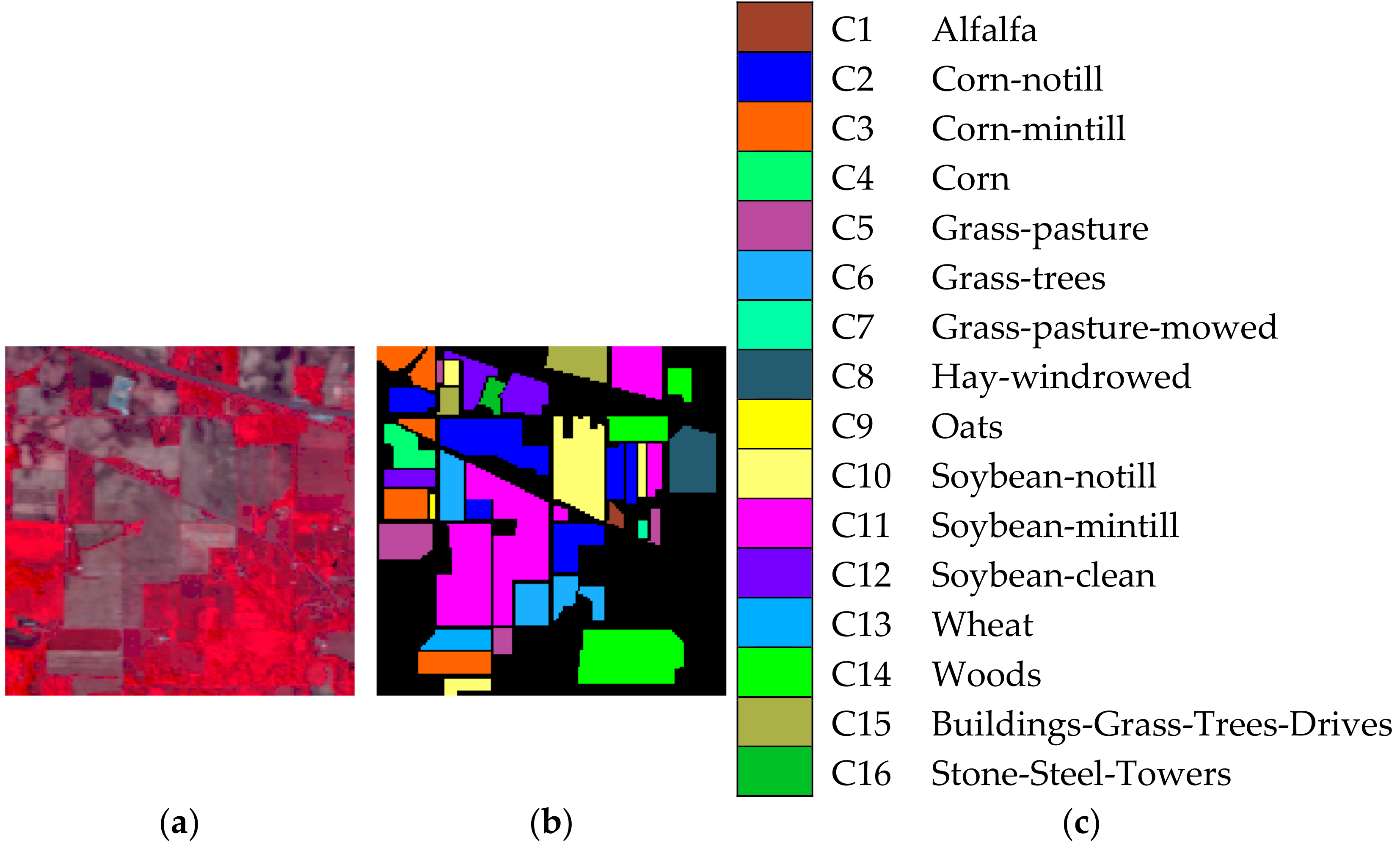
Indian Pines image was the first and famous testing data for hyperspectral image classification, which was obtained by AVIRIS sensors in 1992. The image of Indian Pines includes $145\times 145$ pixels and 220 spectral bands covering the range of 0.4 to 2.5 μm, which shows a mixed agricultural/forest area in northwestern Indiana, America. There are 16 inclusive classes in the available ground-truth map such as alfalfa, corn-mintill, soybean-nottill, etc., which are remarked as C1–C16. Figure 1a–c shows the false color image, ground-truth image, and reference map, respectively.

• Pavia University scene

Figure 1. Indian Pines image. (a) False color image. (b) Ground truth image. (c) reference map.

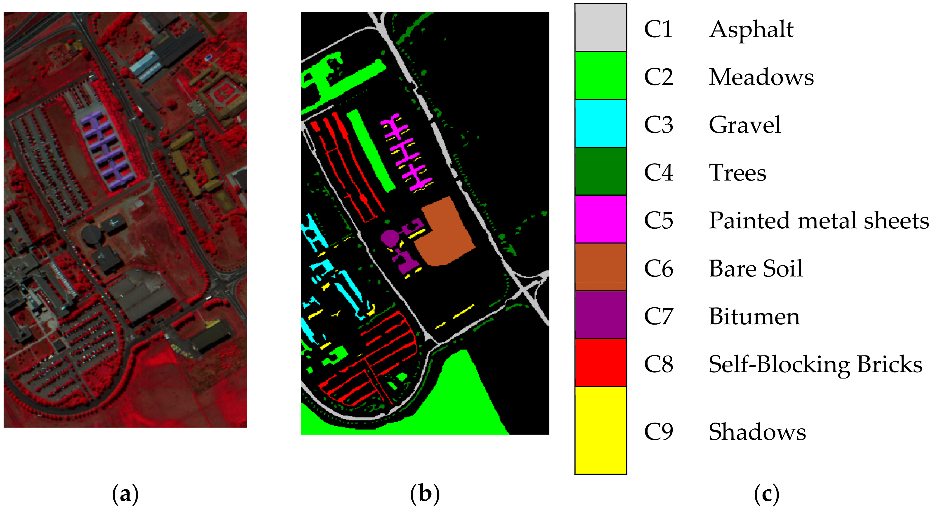
In 2003, the ROSIS sensor collected the Pavia University scene. The scene of Pavia University includes $610\times 340$ pixels and consists of 103 spectral bands with the wavelength varying with 0.43 to 0.86 μm. There are nine available inclusive classes in the ground-truth map including asphalt, meadows, gravel, etc. The classes in this scene are remarked as C1–C9 in the experimental results. Figure 2a–c shows the false color scene, ground-truth image, and reference map of the Pavia University scene, respectively.

• Salinas image

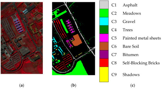
Figure 2. Pavia University scene. (a) False color image. (b) Ground truth image. (c) Reference map.

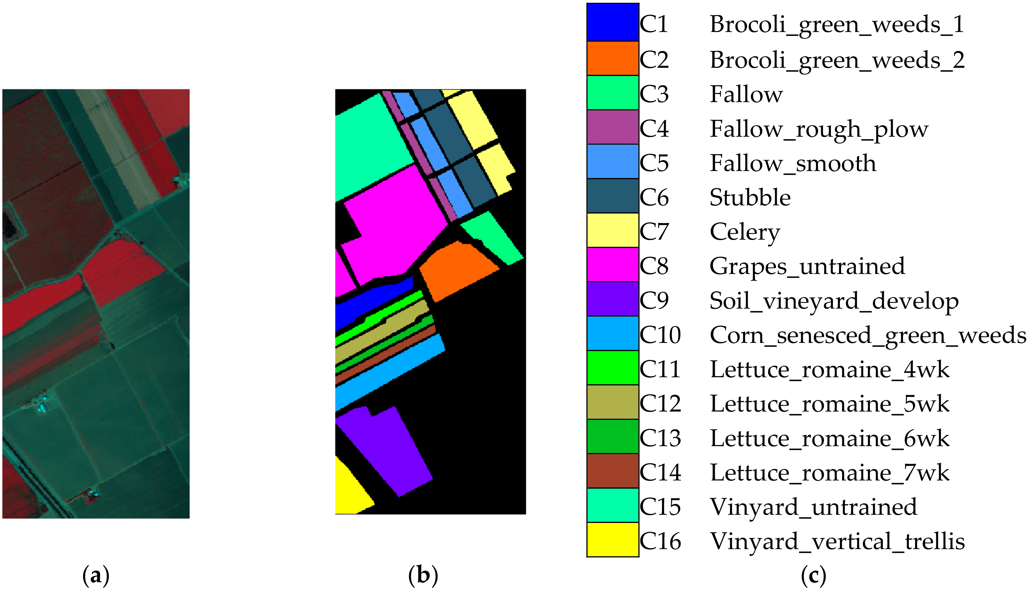
The Salinas image was collected in Salinas Valley, California, USA by AVIRIS. The image of Salinas included $512\times 217$ pixels and 224 spectral bands. Those bands that were absorbed by water were discarded in our experiments. The false color scene is shown in Figure 3a. As is shown in Figure 3b,c, the ground-truth map and reference map included 16 classes such as fallow, stubble, celery, etc. The classes here are remarked as C1–C16.

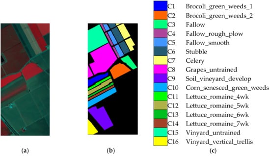
Figure 3. Salinas image. (a) False color image. (b) Ground truth image. (c) Reference map.

4.1.2. Evaluation Criteria

Three evaluation criteria were adopted to judge the effectiveness of each model.

• Overall Accuracy, OA

The overall classification accuracy can visually display the classification results by counting the number of samples classified correctly. The calculation method is the following expression:

$$P_{\mathrm{OA}}=\frac{1}{N}{\displaystyle \sum _{i=1}^n{m}_{ii}}$$

(25)

where $N$ represents the total number of samples and $m_{ii}$ represents the number of samples classified into correct class $i$.

• Average Accuracy, AA

$$P_{\mathrm{AA}}=\frac{1}{N}{\displaystyle \sum _{i=1}^n{P}_{\mathrm{CA}}}$$

(26)

where $P_{\mathrm{CA}}=m_{ii}/N_i$ represents the classification results of single class. AA means the proportion of samples that are successfully classified to their class in the total number of samples in that class. AA is equal to OA when the number of each class is equal to each other.

• Kappa Coefficient

$$K=\frac{N\times {\displaystyle \sum _{i=1}^n{m}_{ii}-{\displaystyle \sum _{i=1}^n{N}_i\times m_{ii}}}}{N^2-{\displaystyle \sum _{i=1}^n{N}_i\times m_{ii}}}$$

(27)

The larger the value of $K$, the higher the consistency between the classified image and original image.

4.1.3. Comparative Algorithms

• TSVM: Transductive Support Vector Machine algorithm [3].
• LGC: The Local and Global Consistency graph-based algorithm [50].
• LPA: the original Label Propagation Algorithm [5].
• LPAPCC: the original Label Propagation Algorithm combined with Particle Cooperation and Competition without the novel graph construction mentioned in Section 3.1.

4.2. Classification of Hyperspectral Images

With the purpose of estimating the performance of our proposed CLPPCC algorithm, several related algorithms were used for comparative experiments such as TSVM, LGC, and LPA. To highlight the importance of the novel graph construction approach on the increased classification performance, we also compared the performance of our proposal and label propagation algorithm combined with particle competition and cooperation (LPAPCC), which do not use the novel graph construction to construct the graph, that is, LPA was only optimized by particle competition and cooperation. Before classifying, aiming at eliminating the redundant and noisy information simultaneously, three hyperspectral datasets were preprocessed by the approach named image fusion and recursive filtering feature (IFRF). IFRF is an effective and powerful feature extraction method. The basic ideas of IFRF are as follows: First, the hyperspectral image is divided into several subsets of adjacent hyperspectral bands. Then, the bands in each subset are fused together by averaging, which is one of the simplest image fusion methods. Finally, the fused frequency band is filtered recursively in the transform domain to obtain the final features for classification. For each hyperspectral dataset we used in the experiments, the training set was composed of 30% samples randomly selected from each class, and the rest of the available samples made up the testing set. Among the training set, it was divided into the labeled set and unlabeled set. For the Indian Pines image dataset, the labeled set was made up of 10% randomly selected samples from each class in the training set, and the remaining samples were defined as the unlabeled set without labels. For the Pavia university scene dataset, the size for the percentage of the labeled set was set to 5%. For the Salinas image dataset, the size for the percentage of the labeled set was set to 2%. Considering the difference between the classes whose total sample number was a few, a minimum threshold was set to five for each class in both the training set and testing set. That is, regardless of the percentage of the selected samples, each class had at least five samples in the training set and labeled set. Each experiment obeyed the above sample division rules. Table 1 shows the distribution of each sample set. Among them, the labeled set and unlabeled set are represented by $\mathrm{L}$ and $\mathrm{U}$, respectively. Here, AA, OA, and kappa coefficient were introduced as evaluation criteria to assess the effectiveness of the models here. To reduce the impact of randomness on the results, the final record result adopted the average result of 10 repeated runs for each hyperspectral dataset and each model.

Table 1. Training and testing samples for the three hyperspectral images.

Class	Indian Pines Image				Pavia University Scene				Salinas Image
	Train		Test	Sample No.	Train		Test	Sample No.	Train		Test	Sample No.
	L	U			L	U			L	U
C1	5	8	33	46	99	1890	4642	6631	12	590	1407	2009
C2	42	386	1000	1428	279	5315	13,055	18,649	22	1095	2609	3726
C3	24	225	581	830	31	598	1470	2099	11	581	1384	1976
C4	7	64	166	237	45	874	2145	3064	8	410	976	1394
C5	14	130	339	483	20	383	942	1345	16	787	1875	2678
C6	21	198	511	730	75	1433	3521	5029	23	1164	2772	3959
C7	5	3	20	28	19	380	931	1330	21	1052	2506	3579
C8	14	129	335	478	55	1049	2578	3682	67	3314	7890	11,271
C9	5	1	14	20	14	270	663	947	37	1823	4343	6203
C10	29	262	681	972	-	-	-	-	19	964	2295	3278
C11	73	663	1719	2455	-	-	-	-	6	314	748	1068
C12	17	160	416	593	-	-	-	-	11	567	1349	1927
C13	6	55	144	205	-	-	-	-	5	269	642	916
C14	37	342	886	1265	-	-	-	-	6	315	749	1070
C15	11	104	271	386	-	-	-	-	43	2137	5088	7268
C16	5	22	66	93	-	-	-	-	10	532	1265	1807
Total	315	2752	7182	10,249	637	12,192	29,947	42,776	317	15,914	37,898	54,129

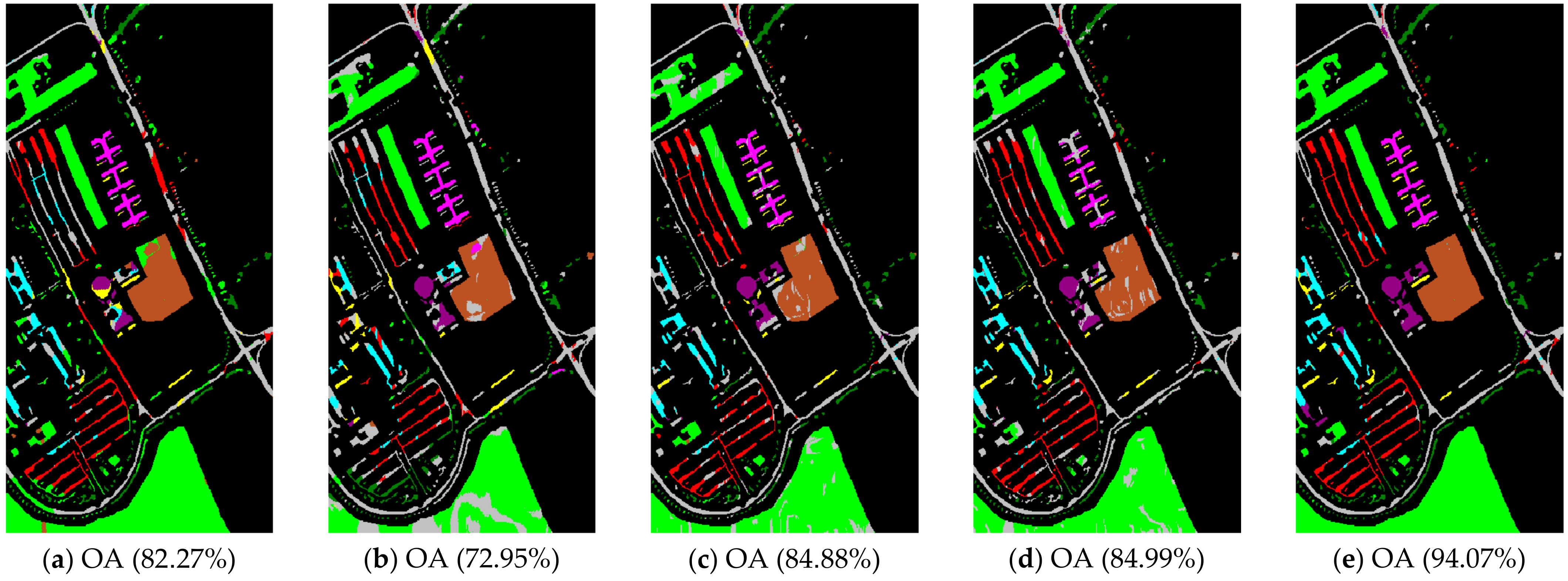
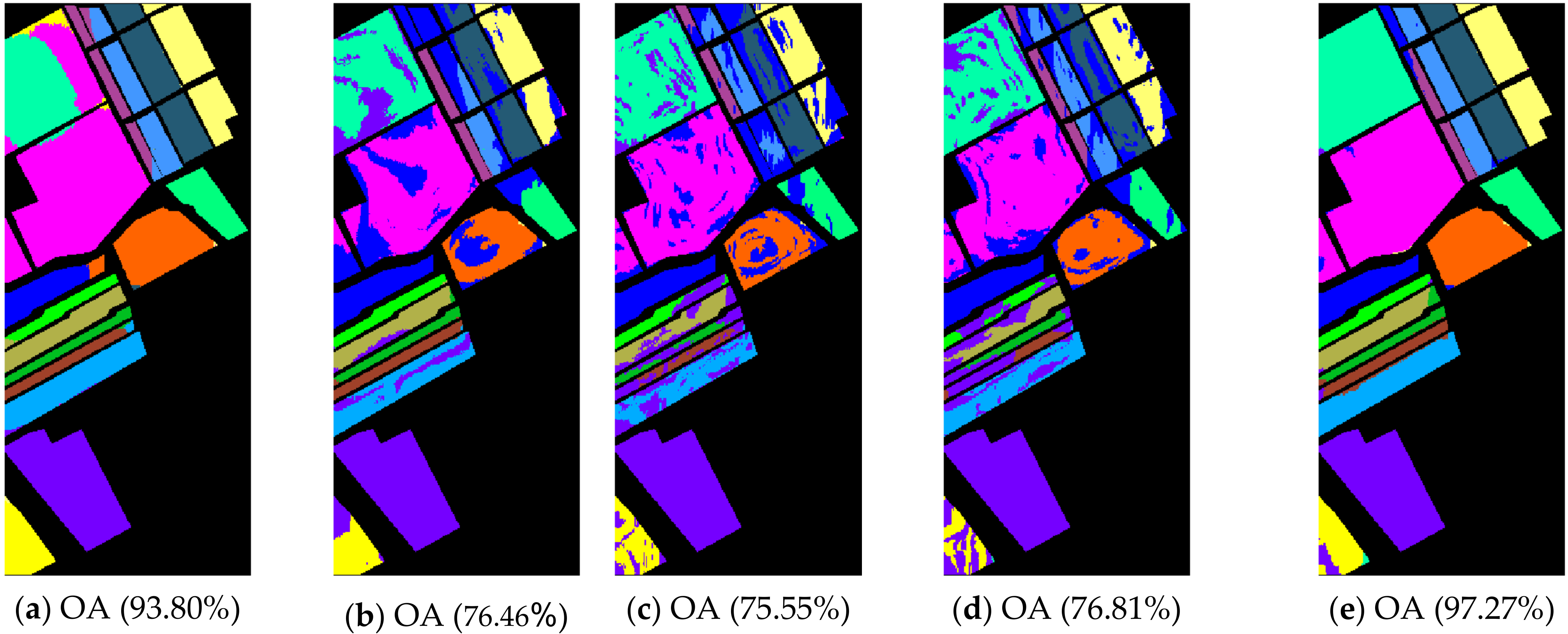
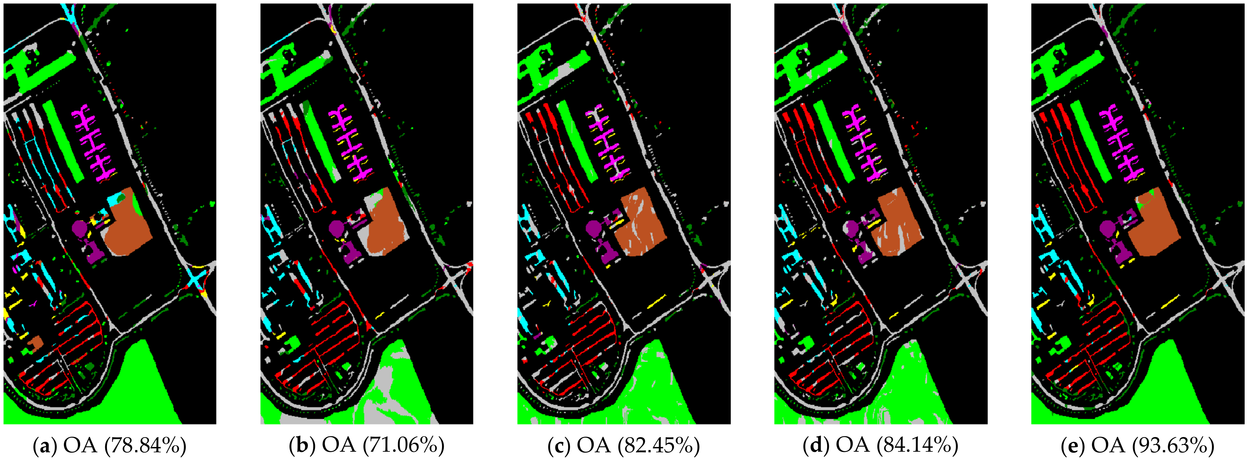
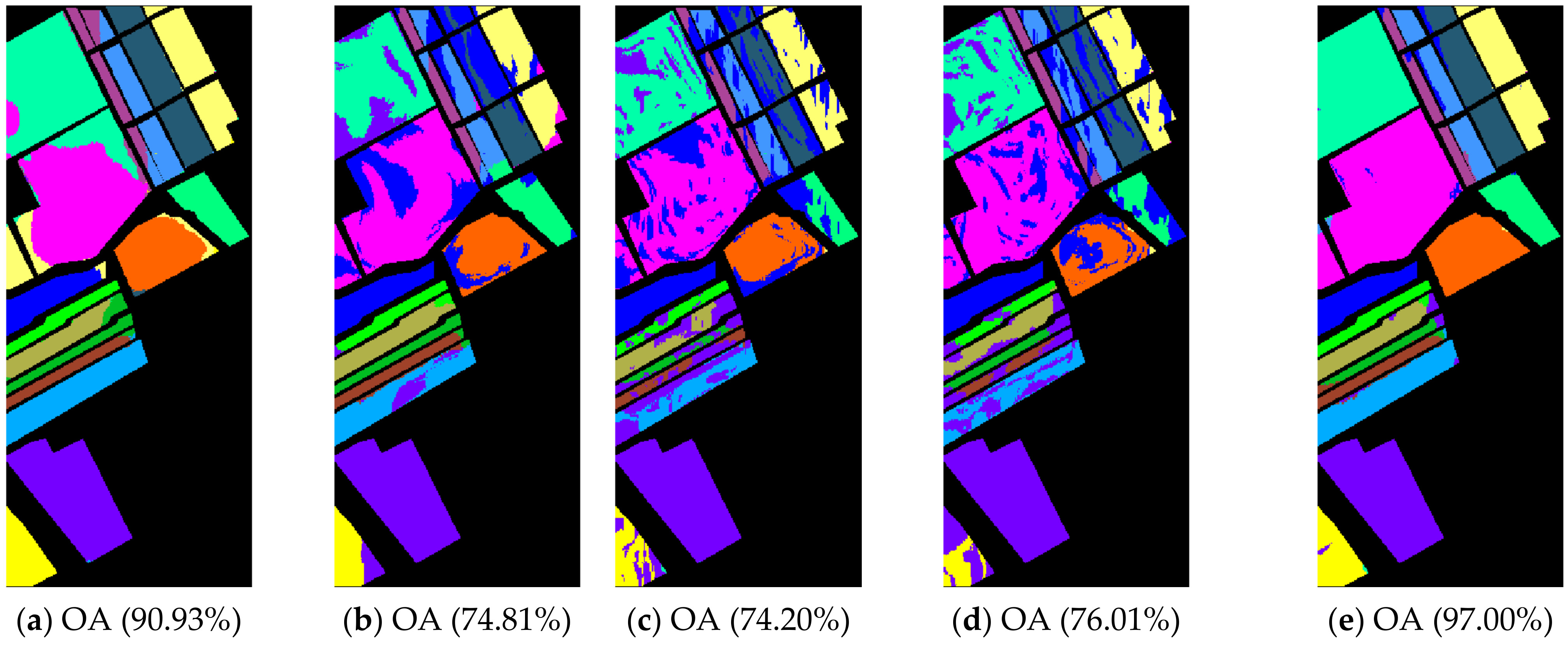
The class-specific accuracies are given in Table 2, Table 3 and Table 4. We can observe the results obtained by each algorithm including AAs, OAs, and Kappa coefficients in three hyperspectral datasets, respectively. For the purpose of analyzing the impact of the neighborhood size $k$, which plays an important role in calculating the affinity matrix $A$, we set up a comparative experiment for each comparison algorithm and our proposal when $k$ was 5 and 10, respectively (see Table 2, Table 3 and Table 4). The best classification results among the various algorithms are in bold. In order to show and compare the classification performance intuitively, the predicted classification maps of the Indian Pines, Pavia University, and Salinas Valley datasets can be clearly observed in Figure 4, Figure 5 and Figure 6, respectively. In Figure 4, Figure 5 and Figure 6, the neighborhood size $k$ was set to five.

Table 2. Indian Pines image classification results.

Method	TSVM	LGC	LPA	LPAPCC	CLPPCC	LPA	LPAPCC	CLPPCC
			$k=5$			$k=10$
C1	0.7251	0.4371	0.0478	0.0547	0.6310	0.8030	0.8126	0.9512
C2	0.8698	0.5140	0.9421	0.9587	0.9357	0.9290	0.9062	0.9200
C3	0.7214	0.5599	0.9326	0.9228	0.9492	0.8795	0.8828	0.9569
C4	0.8806	0.4205	0.9310	0.9574	0.8955	0.9246	0.9313	0.9700
C5	0.9737	0.8059	0.9955	0.9851	0.9729	0.9693	0.9906	0.9783
C6	0.9440	0.7727	0.9758	0.9870	0.9758	0.9671	0.9700	0.9765
C7	0.3597	0.4289	0.6609	0.5325	0.6898	0.4356	0.4244	0.5610
C8	0.9983	0.9413	1	1	1	1	1	1
C9	0.5356	0.1723	0.8180	0.8862	0.7085	0.7788	0.9028	0.9375
C10	0.8255	0.5348	0.9337	0.9360	0.8943	0.9166	0.9192	0.9466
C11	0.8613	0.5228	0.9599	0.9634	0.9607	0.9404	0.9447	0.9656
C12	0.6773	0.4165	0.9214	0.9344	0.9069	0.8932	0.8835	0.9121
C13	0.9806	0.8050	0.9965	0.9970	0.9990	0.9950	0.9955	1
C14	0.9867	0.8388	0.9977	0.9936	0.9799	0.9840	0.9894	0.9984
C15	0.9345	0.4765	0.9511	0.9522	0.9592	0.9520	0.9582	0.9012
C16	0.9757	0.9906	0.9871	0.9780	0.9457	0.9853	0.9874	0.9886
OA	0.8648	0.6188	0.8768	0.8886	0.9439	0.9342	0.9350	0.9571
AA	0.8281	0.6023	0.8682	0.8776	0.9002	0.8971	0.9062	0.9353
Kappa	0.8458	0.5534	0.8607	0.8741	0.9361	0.9249	0.9258	0.9511

Table 3. Pavia University scene classification results.

Method	TSVM	LGC	LPA	LPAPCC	CLPPCC	LPA	LPAPCC	CLPPCC
			$k=5$			$k=10$
C1	0.7126	0.5135	0.5332	0.5335	0.8723	0.8943	0.8982	0.9077
C2	0.9123	0.9198	0.9917	0.9915	0.9886	0.9859	0.9868	0.9905
C3	0.6837	0.6265	0.8954	0.9297	0.8833	0.8702	0.8607	0.8473
C4	0.8198	0.4756	0.9695	0.9777	0.8823	0.9749	0.9610	0.9071
C5	0.9572	0.8932	0.9960	0.9977	0.9853	0.9964	0.9981	0.9960
C6	0.8869	0.9445	0.9949	0.9960	0.9932	0.9839	0.9851	0.9894
C7	0.7080	0.6068	0.9251	0.9059	0.8782	0.8297	0.8551	0.8651
C8	0.6626	0.5431	0.8738	0.8851	0.8676	0.8291	0.8224	0.8543
C9	0.4501	0.2614	0.8894	0.9443	0.8652	0.8439	0.8440	0.8632
OA	0.8227	0.7295	0.8488	0.8499	0.9407	0.9420	0.9425	0.9454
AA	0.7548	0.6427	0.8966	0.9068	0.9129	0.9120	0.9124	0.9134
Kappa	0.7626	0.6502	0.8005	0.8020	0.9213	0.9230	0.9237	0.9276

Table 4. Salinas image classification results.

Method	TSVM	LGC	LPA	LPAPCC	CLPPCC	LPA	LPAPCC	CLPPCC
			$k=5$			$k=10$
C1	0.9378	0.1983	0.2134	0.2174	0.7418	0.8827	0.8830	0.9975
C2	0.9750	1	1	1	1	1	1	1
C3	0.9747	0.9877	0.9971	0.9979	0.9977	0.9918	0.9952	0.9740
C4	0.8457	0.9349	0.9922	0.9900	0.9708	0.9782	0.9837	0.9943
C5	0.9696	0.9384	0.9989	0.9978	1	0.9871	0.9957	0.9621
C6	0.9947	1	1	1	0.9957	0.9999	1	0.9962
C7	0.9649	0.9783	0.9933	0.9956	0.9930	0.9891	0.9880	0.9972
C8	0.9250	0.9944	0.9994	0.9996	0.9998	0.9993	0.9993	0.9945
C9	0.9940	0.6112	0.5211	0.5459	0.9421	0.9640	0.9704	0.9915
C10	0.9827	0.9916	0.9974	0.9948	0.9955	0.9923	0.9899	0.9558
C11	0.9859	1	1	1	0.9797	1	1	1
C12	0.9731	0.9761	0.9937	0.9972	1	0.9876	0.9784	0.9675
C13	0.8525	0.9619	0.9970	0.9927	0.9360	0.9370	0.9618	0.9718
C14	0.9383	0.9082	0.9684	0.9815	0.8646	0.9781	0.9847	0.9777
C15	0.8584	0.9978	0.9992	0.9991	0.9931	0.9974	0.9979	0.9917
C16	0.9796	0.9606	1	1	1	0.9998	0.9980	1
OA	0.9380	0.7646	0.7555	0.7681	0.9727	0.9854	0.9868	0.9881
AA	0.9470	0.9025	0.9169	0.9193	0.9631	0.9803	0.9829	0.9857
Kappa	0.9310	0.7418	0.7269	0.7433	0.9696	0.9837	0.9983	0.9867

Figure 4. Indian Pines image classification results: (a) TSVM; (b) LGC; (c) LPA; (d) LPAPCC; (e) CLPPCC. OA, Overall Accuracy.

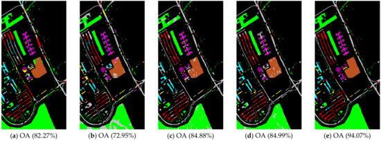
Figure 5. Pavia University scene classification results: (a) TSVM; (b) LGC; (c) LPA; (d) LPAPCC; (e) CLPPCC. OA, Overall Accuracy.

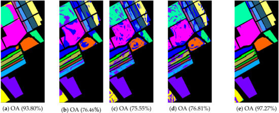
Figure 6. Salinas image classification results: (a) TSVM; (b) LGC; (c) LPA; (d) LPAPCC; (e) CLPPCC. OA, Overall Accuracy.

From the experimental results on the Indian Pines dataset in Table 2, we can observe that TSVM, LGC, LPA ($k=5$), LPAPCC ($k=5$), CLPPCC ($k=5$), LPA ($k=10$), LPAPCC ($k=10$), and CLPPCC ($k=10$) achieved 0, 1, 2, 4, 3, 1, 1, and 9 best-specific accuracies, respectively. Particularly, CLPPCC ($k=10$) achieved 9 best-specific accuracy. From Table 3, we can observe in the results in the Pavia University dataset that TSVM, LGC, LPA ($k=5$), LPAPCC ($k=5$), CLPPCC ($k=5$), LPA ($k=10$), LPAPCC ($k=10$), and CLPPCC ($k=10$) obtained 0, 0, 2, 5, 0, 0, 1, and 1 best class-specific accuracies, respectively. Here, our proposal not only performed well in a large number of class samples, but also performed well in a small number of class samples. For the Salinas dataset, Table 4 shows that TSVM, LGC, LPA ($k=5$), LPAPCC ($k=5$), CLPPCC ($k=5$), LPA ($k=10$), LPAPCC ($k=10$), and CLPPCC ($k=10$) achieved 1, 3, 7, 5, 5, 2, 4, and 6 best class-specific accuracies, respectively. Our proposal CLPPCC performed well in both $k=5$ and $k=10$. The classification results in Figure 4, Figure 5 and Figure 6 show that CLPPCC was more satisfactory than the other compared algorithms when the parameter $k$ was set to five.

From the above experimental results shown in Table 2, Table 3 and Table 4, several conclusions can be summarized. First, CLPPCC ($k=10$) achieved the best OAs, AAs, and kappa coefficients for all three hyperspectral datasets. Second, the classification performance of TSVM, LGC, LPA ($k=5$), and LPAPCC ($k=5$) was not stable in all datasets as they obtained low class-specific accuracies in some small number classes. Third, compared with LPA, LPAPCC and CLPPCC, CLPPCC had the best performance in OAs, AAs, and kappa coefficients in both $k=5$ and $k=10$ for all datasets. LPA and LPAPCC were significantly affected by the value of $k$. When $k$ was set to five, the LPA and LPAPCC performed terribly in a small number of class samples such as C1 in the Indian Pines dataset. When $k$ was set to 10, both LPA, LPAPCC, and CLPPCC improved their performances. CLPPCC was affected by the value of $k$ slightly, and it kept good performance regardless of what the value of $k$ was. The reason why it worked well is because the graph construction approach we used could build a graph that closely related to the samples. Unlike the traditional KNN graph construction, our approach was less affected by the value of $k$. Fourth, compared with LPA and LPAPCC, LPAPCC performed better than LPA in both $k=5$ and $k=10$ for all datasets as it benefitted from the particle competition and cooperation mechanism, which could remark on the misclassified labels from unlabeled samples and could achieve great effectiveness even though there were some misclassified labels in the training process.

4.3. Running time

We recorded and analyzed the average running time of each model in seconds on the three hyperspectral datasets in Table 5. The running time in Table 5 shows that the execution time of LPA ($k=10$), LPAPCC ($k=10$), and CLPPCC ($k=10$) was slightly longer than LPA ($k=5$), LPAPCC ($k=5$) and CLPPCC ($k=5$). It can be seen from Table 2, Table 3 and Table 4 that when the value of $k$ was larger, the higher the overall accuracy obtained. However, we can observe from Table 5 that the running time slowed down as the value of $k$ increased from five to 10. Next, although our proposal CLPPCC was slower than LPA, the classification performance of CLPPCC was better than LPA. This is because the PCC mechanism needs to remark and modifies the misclassified labels in unlabeled samples, and the cost of running time is exchanged for an increase in class-specific accuracy, OAs, AAs, and kappa coefficients. Then, it is worth saying that although the OAs of TSVM was not the best when compared to other algorithms, the running time of TSVM was the fastest among the label propagation algorithms. The running time of LGC was as fast as TSVM, but the performance of LGC was worse than that of TSVM.

Table 5. The running time (in seconds) of CLPPCC and the comparative algorithms on HSIs datasets.

Method	TSVM	LGC	LPA	LPAPCC	CLPPCC	LPA	LPAPCC	CLPPCC
			$k=5$			$k=10$
Indian Pines images	4.51	6.40	28.41	36.78	32.07	30.39	39.18	49.82
Pavia University scene	14.49	132.65	640.89	807.4	884.61	651.20	828.54	958.87
Salinas image	29.34	213.57	1086.87	1897.48	1321.87	1352.86	2069.80	1432.51

4.4. Robustness of the Proposed Method

The effectiveness of our proposed CLPPCC algorithm was appraised in several experiments above. In this section, we analyzed the robustness of our proposal and other comparison algorithms in order to evaluate the superiority of our proposal. We compared our method with alternatives in different sizes of labeled samples and noise situation and the experimental results indicated the robustness of our proposal. Here, the parameter $k$ was set to five.

4.4.1. Labeled Size Robustness

Several experiments with different size of labeled samples were performed in this section. To reduce randomness, we picked the average results of 10 runs repeatedly as the final record result for each hyperspectral dataset. Figure 7 shows the overall classification accuracy of our proposal and four alternatives in different sizes of labeled samples. The labeled samples percentage was 5%, 10%, 12%, 14%, and 16% for the Indian Pines dataset. For the Pavia University scene, the percentage of labeled samples was set to 3%, 5%, 7%, 9%, and 11%. The labeled samples percentage for the Salinas image was set to 1%, 2%, 5%, 8%, and 10%.

Figure 7. HSIs Classification accuracy with varying labeled ratio: (a) Indian Pines image; (b) Pavia University scene; and (c) Salinas image.

From Figure 7, it can be simply found that the higher ratio of labeled samples, the better classification accuracy (OAs) that each algorithm achieved. Simultaneously, other evaluation standards such as AAs, kappa coefficients, and class-specific accuracy were enhanced with the increase in the labeled ratio. Note that in most cases, our CLPPCC obtained the best performance of OAs in all three datasets, which indicates the robustness of CLPPACC in various sizes of labeled samples. It is worth noticing that our proposal achieved a higher classification result even if in a low size of labeled samples and the compared algorithms rarely obtained high classification results with a small size of labeled samples.

4.4.2. Noise Robustness

The noise robustness was analyzed in this section. We added 20 dB of Gaussian noise into each hyperspectral dataset. We selected the average results of 10 runs repeatedly as the final recorded result for each hyperspectral dataset to reduce occasionality. Figure 8a,b demonstrates the clean and noisy images, respectively. For the purpose of showing the impact of noise in overall accuracy, the overall accuracy results of the three hyperspectral datasets are shown in Table 6. Figure 8 shows the false-color clean and noisy image of the Indian Pines image. The classification results of three noisy hyperspectral datasets and their corresponding OA values are shown in Figure 9, Figure 10 and Figure 11. Here, the parameter of $k$ was set to five for all approaches and three HSIs.

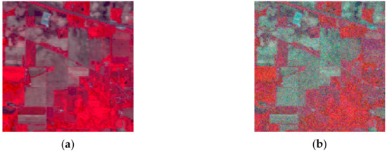
Figure 8. False-color clean and noisy image of the Indian Pines image: (a) clean image; (b) noisy image with Gaussian noise.

Table 6. Classification results with Gaussian noise on three HSIs.

Images		TSVM	LGC	LPA	LPAPCC	CLPPCC
Indian Pines image	OA	0.8269	0.5993	0.8638	0.8822	0.9404
	AA	0.7740	0.5756	0.8736	0.8733	0.8941
	Kappa	0.8026	0.5310	0.8465	0.8669	0.9321
Pavia University scene	OA	0.7884	0.7106	0.8245	0.8414	0.9363
	AA	0.7667	0.6339	0.8880	0.8918	0.9047
	Kappa	0.7120	0.6195	0.7688	0.7908	0.9156
Salinas image	OA	0.9093	0.7481	0.7420	0.7601	0.9700
	AA	0.9191	0.8901	0.9166	0.9174	0.9597
	Kappa	0.8997	0.7239	0.7146	0.7343	0.9666

Figure 9. Noisy Indian Pines image classification results: (a) TSVM; (b) LGC; (c) LPA; (d) LPAPCC; (e) CLPPCC. OA, Overall Accuracy.

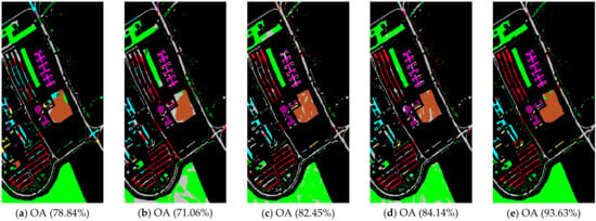
Figure 10. Noisy Pavia University scene classification results: (a) TSVM; (b) LGC; (c) LPA; (d) LPAPCC; (e) CLPPCC. OA, Overall Accuracy.

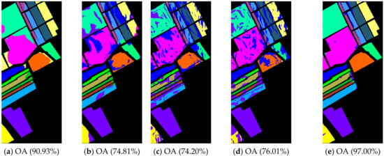
Figure 11. Noisy Salinas image classification results: (a) TSVM; (b) LGC; (c) LPA; (d) LPAPCC; (e) CLPPCC. OA, Overall Accuracy.

From Table 6 and Figure 9, Figure 10 and Figure 11, the performances of all algorithms were affected by the Gaussian noise added into the datasets. The performance degradation of our algorithm was the lowest compared to the others. In addition, the proposed method still kept a high classification result, which indicates that our method is robust.

5. Conclusions

In this paper, we considered a graph-based semi-supervised problem where the usage of unlabeled samples might deteriorate the model performance in HSI classification. In addition, the IFRF method was used to remove the redundant feature information in HSIs. Several conclusions were summarized based on the experiments we performed. First, our proposed CLPPCC was effective for HSI classification. The classification results of CLPPCC were superior to the comparison algorithms among the three hyperspectral datasets. Second, the constrained graph construction approach plays an important role in CLPPCC, which helps CLPPCC keep a high overall accuracy when the percentage of labeled hyperspectral samples is low. Third, the PCC mechanism used in CLPPCC decreases the impact of label noise in an unlabeled hyperspectral dataset. At last, CLPPCC is robust in noise HSIs, and also keeps high overall accuracy with varying labeled ratio.

There are many interesting future works. For instance, the label propagation in our current proposal was based on a classical and initial learning method where several prior strategies and knowledge may be not leveraged. More flexible methods that are able to incorporate the domain knowledge are worth trying in the future.

References

- Deng, C.; Ji, R.; Liu, W.; Tao, D.; Gao, X. Visual Reranking through Weakly Supervised Multi-graph Learning. In Proceedings of the 2013 IEEE International Conference on Computer Vision, Sydney, Australia, 1–8 December 2013; pp. 2600–2607. [Google Scholar]
- Vanegas, J.A.; Escalante, H.J.; González, F.A. Scalable multi-label annotation via semi-supervised kernel semantic embedding. Pattern Recognit. Lett. 2019, 123, 97–103. [Google Scholar] [CrossRef]
- Joachims, T. Transductive inference for text classification using support vector machines. In Proceedings of the Sixteenth International Conference on Machine Learning, Bled, Slovenia, 27–30 June 1999; pp. 200–209. [Google Scholar]
- Blum, A.; Mitchell, T. Combining labeled and unlabeled data with co-training. In Proceedings of the 11th Annual Conference on Computational Learning Theroy, Madison, WI, USA; 1998; pp. 92–100. [Google Scholar]
- Zhu, X.J.; Zoubin, Z. Learning from Labeled and Unlabeled Data with Label Propagation; Carnegie Mellon Univerisity: Pittsburgh, PA, USA, 2002. [Google Scholar]
- Berthelot, D.; Carlini, N.; Goodfellow, L.; Oliver, A.; Papernot, N.; Raffel, C. Mixmatch: A holistic approach to semi-supervised learning. arXiv 2020, arXiv:1905.02249. [Google Scholar]
- Sohn, K.; Berthelot, D.; Li, C.; Zhang, Z.; Carlini, N.; Cubuk, E.; Kurakin, A.; Zhang, H.; Raffel, C. Fixmatch: Simplifying semi-supervised learning with consistency and confidence. arXiv 2020, arXiv:2001.07685. [Google Scholar]
- Igor, S. Semi-supervised neural network training method for fast-moving object detection. In Proceedings of the 2018 14th Symposium on Neural Networks and Applications (NEUREL), Belgrade, Serbia, 20–21 November 2018; pp. 1–6. [Google Scholar]
- Hoang, T.; Engin, Z.; Lorenza, G.; Paolo, D. Detecting mobile traffic anomalies through physical control channel fingerprinting: A deep semi-supervised approach. IEEE Access 2019, 7, 152187–152201. [Google Scholar]
- Tokuda, E.K.; Ferreira, G.B.A.; Silva, C.; Cesar, R.M. A novel semi-supervised detection approach with weak annotation. In Proceedings of the 2018 IEEE Southwest Symposium on Image Analysis and Interpretation (SSIAI), Las Vegas, NV, USA, 8–10 April 2018; pp. 129–132. [Google Scholar]
- Chen, G.; Liu, L.; Hu, W.; Pan, Z. Semi-Supervised Object Detection in Remote Sensing Images Using Generative Adversarial Networks. In Proceedings of the IGARSS 2018—2018 IEEE International Geoscience and Remote Sensing Symposium, Valencia, Spain, 22–27 July 2018; Institute of Electrical and Electronics Engineers: Piscataway, NJ, USA, 2018; pp. 2503–2506. [Google Scholar]
- Zu, B.; Xia, K.; Du, W.; Li, Y.; Ali, A.; Chakraborty, S. Classification of Hyperspectral Images with Robust Regularized Block Low-Rank Discriminant Analysis. Remote Sens. 2018, 10, 817. [Google Scholar] [CrossRef]
- Liu, C.; Li, J.; He, L. Superpixel-Based Semisupervised Active Learning for Hyperspectral Image Classification. IEEE J. Sel. Top. Appl. Earth Obs. Remote Sens. 2018, 12, 1–14. [Google Scholar] [CrossRef]
- Shi, C.; Lv, Z.; Yang, X.; Xu, P.; Bibi, I. Hierarchical Multi-View Semi-supervised Learning for Very High-Resolution Remote Sensing Image Classification. Remote Sens. 2020, 12, 1012. [Google Scholar] [CrossRef]
- Zhou, S.; Xue, Z.; Du, P. Semisupervised Stacked Autoencoder With Cotraining for Hyperspectral Image Classification. IEEE Trans. Geosci. Remote Sens. 2019, 57, 3813–3826. [Google Scholar] [CrossRef]
- Ahmadi, S.; Mehreshad, N. Semisupervised classification of hyperspectral images with low-rank representation kernel. J. Opt. Soc. Am. A 2020, 37, 606–613. [Google Scholar] [CrossRef] [PubMed]
- Mukherjee, S.; Cui, M.; Prasad, S. Spatially Constrained Semisupervised Local Angular Discriminant Analysis for Hyperspectral Images. IEEE J. Sel. Top. Appl. Earth Obs. Remote Sens. 2017, 11, 1203–1212. [Google Scholar] [CrossRef]
- Mohanty, R.; Happy, S.L.; Routray, A. A Semisupervised Spatial Spectral Regularized Manifold Local Scaling Cut with HGF for Dimensionality Reduction of Hyperspectral Images. IEEE Trans. Geosci. Remote Sens. 2019, 57, 3423–3435. [Google Scholar] [CrossRef]
- Wu, Y.; Mu, G.; Qin, C.; Miao, Q.-G.; Ma, W.; Zhang, X. Semi-Supervised Hyperspectral Image Classification via Spatial-Regulated Self-Training. Remote Sens. 2020, 12, 159. [Google Scholar] [CrossRef]
- Hu, Y.; An, R.; Wang, B.; Xing, F.; Ju, F. Shape Adaptive Neighborhood Information-Based Semi-Supervised Learning for Hyperspectral Image Classification. Remote Sens. 2020, 12, 2976. [Google Scholar] [CrossRef]
- Triguero, I.; García, S.; Herrera, F. Self-labeled techniques for semi-supervised learning: Taxonomy, software and empirical study. Knowl. Inf. Syst. 2015, 42, 245–284. [Google Scholar] [CrossRef]
- Wang, D.; Nie, F.; Huang, H. Large-scale adaptive semi-supervised learning via unified inductive and transductive model. In Proceedings of the 20th ACM SIGKDD International Conference on Knowledge Discovery and Data Mining, New York, NY, USA, 24–27 August 2014; pp. 482–491. [Google Scholar]
- Abu-Aisheh, Z.; Raveaux, R.; Ramel, J.-Y. Efficient k-nearest neighbors search in graph space. Pattern Recognit. Lett. 2020, 134, 77–86. [Google Scholar] [CrossRef]
- Yang, X.; Deng, C.; Liu, X.; Nie, F. New -norm relaxation of multi-way graph cut for clustering. In Proceedings of the Thirty-Second AAAI Conference on Artificial Intelligence, New Orleans, LA, USA, 2–7 February 2018. [Google Scholar]
- Nie, F.; Wang, X.; Jordan, M.; Huang, H. The constrained Laplacian rank algorithm for graph-based clustering. In Proceedings of the Thirtieth AAAI Conference on Artificial Intelligence, Phoenix, AZ, USA, 12–17 February 2016; AAAI Press: New Orleans, LA, USA, 2016. [Google Scholar]
- Breve, F.; Zhao, L.; Quiles, M.; Pedrycz, W.; Liu, C.-M. Particle Competition and Cooperation in Networks for Semi-Supervised Learning. IEEE Trans. Knowl. Data Eng. 2011, 24, 1686–1698. [Google Scholar] [CrossRef]
- Breve, F.A.; Zhao, L. Particle Competition and Cooperation to Prevent Error Propagation from Mislabeled Data in Semi-supervised Learning. In Proceedings of the 2012 Brazilian Symposium on Neural Networks, Curitiba, Brazil, 20–25 October 2012; pp. 79–84. [Google Scholar]
- Breve, F.A.; Zhao, L.; Quiles, M.G. Particle competition and cooperation for semi-supervised learning with label noise. Neurocomputing 2015, 160, 63–72. [Google Scholar] [CrossRef]
- Tan, K.; Zhang, J.; Du, Q.; Wang, X. GPU Parallel Implementation of Support Vector Machines for Hyperspectral Image Classification. IEEE J. Sel. Top. Appl. Earth Obs. Remote Sens. 2015, 8, 4647–4656. [Google Scholar] [CrossRef]
- Gao, L.; Plaza, L.; Khodadadzadeh, M.; Plaza, J.; Zhang, B.; He, Z.; Yan, H. Subspace-Based Support Vector Machines for Hyperspectral Image Classification. IEEE Geosci. Remote Sens. Lett. 2014, 12, 349–353. [Google Scholar] [CrossRef]
- Liu, L.; Huang, W.; Liu, B.; Shen, L.; Wang, C. Semisupervised Hyperspectral Image Classification via Laplacian Least Squares Support Vector Machine in Sum Space and Random Sampling. IEEE J. Sel. Top. Appl. Earth Obs. Remote Sens. 2018, 11, 4086–4100. [Google Scholar] [CrossRef]
- Haut, J.M.; Paoletti, M.E.; Plaza, J.; Plaza, L.; Plaza, A. Active Learning with Convolutional Neural Networks for Hyperspectral Image Classification Using a New Bayesian Approach. IEEE Trans. Geosci. Remote Sens. 2018, 56, 6440–6461. [Google Scholar] [CrossRef]
- Priya, T.; Prasad, S.; Wu, H. Superpixels for Spatially Reinforced Bayesian Classification of Hyperspectral Images. IEEE Geosci. Remote Sens. Lett. 2015, 12, 1071–1075. [Google Scholar] [CrossRef]
- Ham, J.; Chen, Y.; Crawford, M.; Ghosh, J. Investigation of the random forest framework for classification of hyperspectral data. IEEE Trans. Geosci. Remote Sens. 2005, 43, 492–501. [Google Scholar] [CrossRef]
- Zhang, Y.; Cao, G.; Li, X.; Wang, B. Cascaded Random Forest for Hyperspectral Image Classification. IEEE J. Sel. Top. Appl. Earth Obs. Remote Sens. 2018, 11, 1082–1094. [Google Scholar] [CrossRef]
- Peerbhay, K.Y.; Mutanga, O.; Ismail, R. Random Forests Unsupervised Classification: The Detection and Mapping of Solanum mauritianum Infestations in Plantation Forestry Using Hyperspectral Data. IEEE J. Sel. Top. Appl. Earth Obs. Remote Sens. 2015, 8, 3107–3122. [Google Scholar] [CrossRef]
- Tu, B.; Huang, S.; Fang, L.; Zhang, G.; Wang, J.; Zheng, B. Hyperspectral Image Classification via Weighted Joint Nearest Neighbor and Sparse Representation. IEEE J. Sel. Top. Appl. Earth Obs. Remote Sens. 2018, 11, 4063–4075. [Google Scholar] [CrossRef]
- Blanzieri, E.; Melgani, F. Nearest Neighbor Classification of Remote Sensing Images with the Maximal Margin Principle. IEEE Trans. Geosci. Remote Sens. 2008, 46, 1804–1811. [Google Scholar] [CrossRef]
- Zhao, Y.; Su, F.; Fengqin, Y. Novel Semi-Supervised Hyperspectral Image Classification Based on a Superpixel Graph and Discrete Potential Method. Remote Sens. 2020, 12, 1528. [Google Scholar] [CrossRef]
- Jamshidpour, N.; Safari, A.; Homayouni, S. A GA-Based Multi-View, Multi-Learner Active Learning Framework for Hyperspectral Image Classification. Remote Sens. 2020, 12, 297. [Google Scholar] [CrossRef]
- Zhang, Y.; Cao, G.; Li, X.; Wang, B.; Fu, P. Active Semi-Supervised Random Forest for Hyperspectral Image Classification. Remote Sens. 2019, 11, 2974. [Google Scholar] [CrossRef]
- Ou, D.; Tan, K.; Du, Q.; Zhu, J.; Wang, X.; Chen, Y. A Novel Tri-Training Technique for the Semi-Supervised Classification of Hyperspectral Images Based on Regularized Local Discriminant Embedding Feature Extraction. Remote Sens. 2019, 11, 654. [Google Scholar] [CrossRef]
- Cui, B.; Xie, X.; Hao, S.; Cui, J.; Lu, Y. Semi-Supervised Classification of Hyperspectral Images Based on Extended Label Propagation and Rolling Guidance Filtering. Remote Sens. 2018, 10, 515. [Google Scholar] [CrossRef]
- Xue, Z.; Du, P.; Su, H.; Zhou, S. Discriminative Sparse Representation for Hyperspectral Image Classification: A Semi-Supervised Perspective. Remote Sens. 2017, 9, 386. [Google Scholar] [CrossRef]
- Xia, J.; Liao, W.; Du, P. Hyperspectral and LiDAR Classification with Semisupervised Graph Fusion. IEEE Geosci. Remote Sens. Lett. 2020, 17, 666–670. [Google Scholar] [CrossRef]
- Cao, Z.; Li, X.; Zhao, L. Semisupervised hyperspectral imagery classification based on a three-dimensional convolutional adversarial autoencoder model with low sample requirements. J. Appl. Remote Sens. 2020, 14, 024522. [Google Scholar] [CrossRef]
- Zhao, W.; Chen, X.; Bo, Y.; Chen, J. Semisupervised Hyperspectral Image Classification with Cluster-Based Conditional Generative Adversarial Net. IEEE Geosci. Remote Sens. Lett. 2020, 17, 539–543. [Google Scholar] [CrossRef]
- Fahime, A.; Mohanmad, K. Improving semisupervised hyperspectral unmixing using spatial correlation under a polynomial postnonlinear mixing model. J. Appl. Remote Sens. 2019, 13, 036512. [Google Scholar]
- Kang, X.; Li, S.; Benediktsson, J.A. Feature Extraction of Hyperspectral Images with Image Fusion and Recursive Filtering. IEEE Trans. Geosci. Remote Sens. 2013, 52, 3742–3752. [Google Scholar] [CrossRef]
- Zhou, D.; Olivier, B.; Thomas, N. Learning with Local and Global Consistency; MIT Press: Cambridge, MA, USA, 2003; pp. 321–328. [Google Scholar]
Publisher’s Note: MDPI stays neutral with regard to jurisdictional claims in published maps and institutional affiliations. |
© 2021 by the authors. Licensee MDPI, Basel, Switzerland. This article is an open access article distributed under the terms and conditions of the Creative Commons Attribution (CC BY) license (http://creativecommons.org/licenses/by/4.0/).