Abstract
China New Generation Doppler Weather Radar (CINRAD) plans to upgrade its hardware and software to achieve polarimetric function. However, the small-magnitude polarimetric measurements were negatively affected by the scattering characteristics of ground clutter and the filter’s response to the ground clutter. This polarimetric contamination was characterized by decreased differential reflectivity (ZDR) and cross-correlation coefficient (ρhv), as well as an increased standard deviation of the differential phase (ΦDP), generating a large-area and long-term observational anomaly for eight polarimetric radars in South China. Considering that outliers simultaneously appeared in the radar mainlobe and sidelobe, the variations in the reflectivity before and after clutter mitigation (ΔZH) and ρhv were used for quantitatively describing the random dispersion caused by mainlobe and sidelobe clutters. The performance of polarimetric algorithms was also reduced by clutter contamination. The deteriorated membership functions in the hydrometeor classification algorithm changed the proportion of classified echoes. The empirical relations of R(ZH, ZDR) and R(KDP) were broken in the quantitative precipitation estimation algorithm and the extra error considerably exceeded the uncertainty caused by the drop-size distribution (DSD) variability of R(ZH). The above results highlighted the negative impact of clutter contamination on polarimetric applications that need to be further investigated.
1. Introduction
The electromagnetic energy emitted by a radar antenna is focused on a solid angle of the antenna center. Even at the edge of the radar mainlobe, this energy can still attain half of its peak intensity. Theoretically, irrespective of whether an object is in or out of the beam width, obvious backscattering will occur under the correct conditions. When the backscatter originates from the terrain or other non-meteorological targets (e.g., buildings and trees), the Rayleigh approximation [1,2] to such returns is not applicable and the phenomenon of ground clutter contamination is observed by weather radars.
To mitigate the negative clutter impact, the identification and suppression algorithms in the radar signal processor were continuously improved. The elliptic filter was initially used to suppress low-frequency clutter signals but the indiscriminate processing of meteorological signals resulted in data missing zero-velocity weather echoes. The Gaussian model adaptive processing (GMAP) filter proposed later uses a Gaussian clutter model and weather model to remove the clutter components and to simultaneously restore the meteorological signals in the frequency domain [3]. A static clutter map was once used in the mitigation scheme of the Weather Surveillance Radar-1988 Doppler (WSR-88D) of the United States (U.S.) to detect the existence of ground clutter for hardware filtering. Then, the clutter mitigation decision algorithm (CMD) was proposed to automatically detect clutter and control the application of the GMAP filter in real-time [4,5]. The Clutter Environment Analysis using Adaptive Processing (CLEAN-AP) filter plans to integrate the filtering and its control into a single algorithm and meet the requirements of staggered-pulse repetition time (PRT) sequences of the WSR-88D radar [6]. Besides the operational application, some novel methods, such as the Bayesian classifier and three-dimensional (3D) discriminant function, have also been proposed to better detect the ground clutter mixed with weather signals [7,8].
For the horizontally polarized reflectivity factor (ZH), the power response of clutter filters has reached −50 dB to ensure enough observational accuracy in current operational weather radars [9]. But for polarimetric measurements (i.e., the differential reflectivity ZDR, differential phase ΦDP, specific differential phase KDP and cross-correlation coefficient ρhv), studies about their filter scheme are relatively rare. When the polarimetric radar receives clutter signals, small differences in the filter response or non-Rayleigh scattering between horizontal and vertical polarizations can result in the polarimetric measurements falling outside the common value range. Some studies used above vulnerable variables and their obvious contaminated characteristics to identify ground clutters [10,11,12]. But what’s the relationship between contaminated pixels and the surrounding terrain? How to quantify this negative influence on polarimetric observations? Answers to these questions are not clear. Furthermore, previous studies showed advantages of polarimetric radar technology in hydrometeor classification (HC) [13,14,15,16] and quantitative precipitation estimation (QPE) [17,18,19,20,21,22,23,24,25,26] and applied it in radar nowcasting [27,28,29]. Considering the algorithm stability is affected in the clutter-contaminated regions, the relevant evaluation is also necessary.
Due to the complex terrain and rapid urbanization in China, the impact of ground clutter on weather radars is becoming a serious issue. Previous studies used the digital elevation model (DEM) to analyze the coverage of China New Generation Doppler Weather Radar (CINRAD) and found that beam blockage is a common occurrence [30,31]. The climatological characteristics of the CINRAD’s beam propagation conditions also proved that radars in the coastal areas (e.g., Pearl River delta) are as vulnerable as those on plateaus to ground clutter contamination [32]. Some studies attempted to fuse satellite and radar products in severely blocked areas over the Tibetan plateau [33,34,35,36,37,38], while the evaluation of clutter blockage and contamination for polarimetric CINRAD has not been carried out.
Since 2016, South China became the first region to operate dual-polarization radars to cope with extreme rainfall [39]. Herein, eight polarimetric CINRADs in South China, upgraded between 2016 and 2018, were used to statistically analyze the polarimetric characteristics and the spatiotemporal distribution of clutter contamination. This article is organized into five sections: Section 2 introduces the instruments and analysis methods; Section 3 presents the quantitative assessment of the polarimetric features of clutter contamination; Section 4 introduces the uncertainty of polarimetric algorithms in clutter-contaminated regions. Finally, Section 5 presents the study’s conclusions.
2. Data and Methodology
Figure 1 illustrates the locations of CINRADs and the surrounding topography in South China. Radars in Guangzhou (GZ), Yangjiang (YJ), Qingyuan (QY), Shaoguan (SG), Shenzhen (SZ), Meizhou (MZ), Shantou (ST) and Zhanjiang (ZJ) completed the polarimetric upgrade between 2016 and 2018, while other radars were scheduled to be upgraded after 2019. Among the eight upgraded radars, the GZ, YJ and ZJ radars are stationed close to the coast with a flat terrain, whereas the QY and SG radars are located in mountainous regions. The topography in South China reveals that the issue of clutter contamination faced by the new polarimetric radars is highly representative for the whole of China.
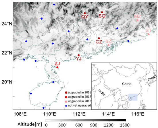
Figure 1.
Distribution of the China New Generation Doppler Weather Radar (CINRAD) stations in South China; grey shading represents the topography; blue shading on the mini-map represents the general position of South China in Asia.
The measurement uncertainty of clutter contamination mainly stems from the anomaly between the two orthogonal channels, which is caused by non-Rayleigh scattering and the filter response in clutter mitigation. Under different atmospheric refraction conditions, the propagation path of the radar beam might be deviated upward or downward. This change further enhances the abovementioned uncertainty. A series of statistical methods are used to objectively evaluate the influence of clutter contamination on long-term observations (1~3 years) of polarimetric radars in South China. The procedures are described as follows—(1) The data accumulation of long-time rainfall. All the rainfall cases are point-to-point averaged to calculate the accumulated data with the same spatial resolution. The random errors and different precipitation characteristics decrease with the increasing accumulative times, highlighting the clutter influence on each pixel; (2) The qualitative identification and description of contaminated regions using accumulated data. According to the spatiotemporal distribution of polarimetric outliers, the extent of clutter contamination can be identified at each elevation tilt. The variation in ZH before and after clutter mitigation (ΔZH) represents the intensity of the clutter signals and is used to qualitatively describe the clutter levels; (3) The quantitative statistics of contaminated regions using entire time series observations. The probability distribution of the polarimetric measurements in different contaminated regions is calculated and compared with that in the pure rain region. Since the polarimetric measurements in pure rain can only appear in a fixed dynamic range (e.g., −0.5 dB < ZDR < 2.5 dB, 0.95 < ρhv < 1.0, 0.0° < SD (ΦDP) < 7.0°), the averaged prior probability of pure rain PRA(Ave) (calculated by the integral of probability density function in the above fixed range) is used to quantify the quality of polarimetric measurements in different clutter levels. Note that only large-scale rainfall cases with more than 50% of the total number of observed pixels can be selected in the dataset for accumulation and statistics. To avoid the sensitivity difference that varies with the distance, the radar minimum detectable reflectivity at the radial end is used as the threshold for all accumulated pixels.
Radar algorithm of HC and QPE are chosen to analyze the clutter influence on algorithm stability. The HC algorithm uses the fuzzy logic approach proposed by Park et al. [13], wherein the echoes are classified into 10 classes: ground clutter or anomalous propagation (GC/AP), biological scatters (BS), dry aggregated snow (DS), wet snow (WS), crystals of various orientations (CR), graupel (GR), big drops (BD), light and moderate rain (RA), heavy rain (HR) and a mixture of rain and hail (RH). The QPE algorithm is an empirical relationship between the radar observations and gauge measurements. Whether the classical relation of R = 0.0196 ZH0.688 or one of the later proposed polarimetric relations of R = 0.0196 ZH0.688 ZDR−3.49, R = 44.5 KDP0.782 and R = 4120 AH1.03 is used, the goal is to reduce the estimation bias introduced by the variability of drop-size distributions (DSD) [40,41,42,43,44]. Considering the large variation of radar measurements in the clutter-contaminated region, the outliers of ZH, ZDR, ρhv and KDP can introduce new uncertainties for the HC and QPE algorithm. Intuitively, this clutter contamination is reflected in the anomalous retrieved rain rate or classified hydrometeors; however, the actual reason is the deteriorated performance of established membership functions and empirical relationships. The evaluation of above algorithms uses long-term statistics of radar products to find the critical factors. The radar retrieved rainfall is directly compared with rain gauges around the radar, while the climate characteristics of hydrometeor classes are used in the HC evaluation due to the lack of suitable observations. All the statistical samples are strictly limited in reasonable ranges to minimize the uncertainty and guarantee the representativeness of the evaluation results.
3. Polarimetric Characteristics of Ground Clutter Contamination and Quantitative Assessment
3.1. Polarimetric Characteristics of Ground Clutter Contamination
Figure 2 shows an example of the horizontal structures of accumulated measurements of the SG radar from 2016 to 2017, including the ZH before and after the clutter mitigation, mitigated ZDR, ρhv and the standard deviation of ΦDP (SD (ΦDP)).
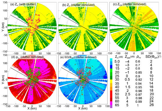
Figure 2.
Horizontal structures of the accumulated measurements of (a) ZH before clutter mitigation, (b) ZH after clutter mitigation, (c) ZDR after clutter mitigation, (d) ρhv after clutter mitigation, (e) standard deviation of ΦDP (SD ΦDP) after clutter mitigation at an elevation angle of 0.5° for the SG radar; the accumulated data were selected from April to October between 2016 and 2017; the black solid line represents the position of the vertical cross section in Figure 3 and the dot circle represents an observation radius multiple of 50 km.
The rainfall characteristics exhibited similarity after two years of accumulation. The ZH and ZDR in most pixels ranged from 30 to 35 dBZ and from 0.5 to 1.0 dB, respectively, with the ρhv typically being greater than 0.98 and the SD (ΦDP) being less than 4°. Due to the mountainous blockage near the SG radar, the anomalous features of ground clutter could be easily discriminated from the meteorological echoes. The full-beam blockage (FBB) of the ground clutter led to pixels without any measurements during the accumulative period in the lower elevations. The partial beam blockage (PBB) phenomena were found in pixels where the ZH along the whole radial component was much weaker (ZH < 30 dBZ) near the FBB. Polarimetric measurements of ρhv and SD (ΦDP) in the PBB region appeared to be similar to the surrounding rainfall region; but serious biases were found in the reflectivity-derived measurements (ZH and ZDR), causing overall difficulties in data applications.
Pixels representing mountain echoes were also observed within a radius of 60 km from the SG radar. The unfiltered ZH reached 45 to 80 dBZ (Figure 2a) and far exceeded the dynamic range of rainfall. This anomalous region almost disappeared after GMAP filtering in Figure 2b, the high values of ΔZH show that the GMAP performed well on the clutter suppression of ZH. However, significant differences were still found in the accumulated polarimetric measurements. The values of ZDR and ρhv decreased to <0.2 dB and <0.9 respectively (Figure 2c–d) and the SD (ΦDP) inversely increased to more than 15° (Figure 2e). Clearly, the efficiency of the current GMAP scheme in suppressing clutter and restoring weather signals was unsuitable for ZDR, ρhv and ΦDP, with a much smaller magnitude, thereby, contaminating the polarimetric measurements.
The vertical cross-sections (Figure 3) are superimposed by the DEM to analyze the relationship between contaminated pixels and the surrounding terrain. The clutter characteristics with both large-ΔZH and the polarimetric outliers near the mountains is defined as the abnormal region resulting from the near-mainlobe ground clutter (MGC). When the altitude of the radar beam reached 2 km away from the mountains, anomalously ZDR, ρhv and ΦDP were still found and associated with low values of ΔZH (less than 1 dB). Considering that the mainlobe of the radar beam was unaffected by the terrain at this altitude, this contamination might originate from the clutter signals received by the radar sidelobe, which is defined as the sidelobe ground clutter (SGC). Both the MGC and SGC regions indicated the negative influence from the mixture of precipitation and clutter signals. Other pixels that neither blocked (FBB, PBB) nor contaminated (MGC, GSC) by clutters are defined as the non-ground clutter (NGC) region and used as the standard samples for comparative analysis.
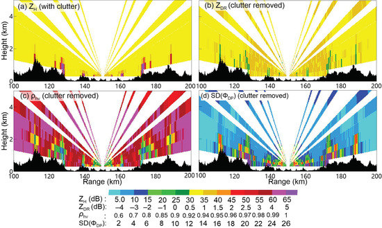
Figure 3.
Vertical structures of the accumulated measurements of (a) ZH before clutter mitigation, (b) ZDR after clutter mitigation, (c) ρhv after clutter mitigation, (d) standard deviation of ΦDP (SD ΦDP) after clutter mitigation at the azimuth between 120° and 300° for the SG radar; Black profiles represent the terrain from the digital elevation model.
3.2. Spatiotemporal Distribution of Ground Clutter Contamination
Using the accumulated data and qualitative definitions, the pixel proportion of the FBB, PBB, MGC, SGC and NGC regions at each elevation tilt was calculated in the histograms of Figure 4 to analyzed the spatiotemporal distribution of ground clutter contamination. The PRA(Ave) in different contaminated regions (represented by the broken lines) was also counted to verify the representation of the accumulated data. The histograms show that the beam blockage was uncommon on radars in South China. A few blocked phenomena can be found in the SG, YJ, ST and ZJ radar along the coast and only 10.7% of the pixels of the SZ radar in the first layer were blocked by ground clutter. The data quality of the above radars was superior in conventional assessments. In contrast, the radial rays of the MZ, SG and QY radar in the mountainous terrain were blocked more severely. The proportion of the blocked pixels increased to 25.1%, 33.2% and 44.3%, respectively, at the first elevation tilt. Only when the elevation angle exceeded 2.4°, did the proportion of the beam blockage decrease by less than 5%.
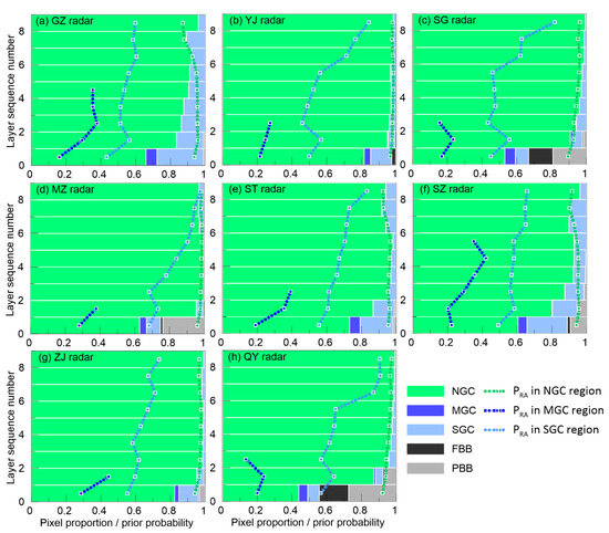
Figure 4.
(a) Histogram of the pixel proportion of different types of ground clutter contamination calculated by the accumulated data of the Guangzhou (GZ) radar. Green, dark blue, light blue, black and gray represent the non-ground clutter (NGC), mainlobe ground clutter (MGC), sidelobe ground clutter (SGC), partial beam blockage (PBB) and full-beam blockage (FBB) regions, respectively. Broken lines in the same colors represent the prior probability of pure rain in different regions during the entire time series of the accumulative period. (b–h) The same as (a) but for the statistical results of the Yangjiang (YJ), Shaoguan (SG), Meizhou (MZ), Shantou (ST), Shenzhen (SZ), Zhanjiang (ZJ) and Qingyuan (QY) radars.
It is surprising that the proportion of MGC and SGC regions was much higher than that of the FBB and PBB regions in most of the accumulated data, suggesting polarimetric contamination to be the primary factor affecting data quality in South China. The PRA in the NGC region was close to 1, whereas the MGC and SGC regions had a much lower prior probability (~0.5 and ~0.2); this demonstrates that the clutter contamination could contribute to numerous polarimetric outliers over a long period. A significant difference in the SGC proportions were found among the eight polarimetric radars in South China. Radars located in the YG, SG, MZ, ZJ and QY stations were less affected by the SGC contamination, with the proportions ranging from 6% to 12% in the first layer and less than 6% at other elevations. In contrast, the proportions of the SGC region in the ST, SZ and GZ radar were much higher than others, reaching 19% to 26% in the first layer, which was ascribed to severe sidelobe contamination.
All accumulated pixels with a PRA less than 0.5 and the terrain height below these outliers were projected to the range-height profiles in Figure 5 to investigate the relationship between the clutter contamination and the terrain around the radar. The common feature among radars with less sidelobe influence (YJ, SG, MZ, ZJ and QY radar) was that all the contaminated pixels were concentrated in a limited spatial distribution. Even for the SG, MZ and QY radars with complex terrain and considerable blockage, the outliers were slightly spread to higher elevations with small proportions. But for the three radars of GZ, ST and SZ near the coast, extensive and continuous polarimetric contamination occurred in most elevations within a radius of 100 km, which demonstrated that abnormal pixels with large proportion and wide spatial distribution had little correlation with the terrain. Considering that the above radars were deployed in the cities with the top population density in Guangdong province, the actual reason might be related to impact of megacities on microwave propagation and needs to be further investigated.
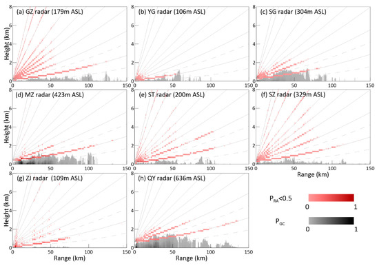
Figure 5.
(a) The range-height distribution of the contaminated polarimetric measurements. The red gradient represents the frequency distribution of the abnormal pixels in the mainlobe ground clutter (MGC) and sidelobe ground clutter (SGC) regions with PRA less than 0.5 and the gray gradient represents the frequency distribution of the terrain height below the outlier points. The gray solid line represents the center of the beam propagation of each elevation under standard atmospheric refractive conditions. The gray dashed line represents the upper and lower boundaries of the half-power beam width of 0.5° elevation. (b–h), the same as (a) but for the statistical results of the YJ, SG, MZ, ST, SZ, ZJ and QY radars.
Therefore, both the beam blockage and polarimetric contamination reflect the negative impact of ground clutter from two individual aspects. The radars located at flat terrain with a low blockage rate were prone to severe contamination (e.g., GZ, ST and SZ) and vice versa (e.g., SG, MZ and QY), proposing high requirements for data application.
3.3. Quantitative Description of Ground Clutter Contamination
Anomalous features of the decreased ZDR and ρhv, as well as the increased SD(ΦDP) were preliminarily found in the MGC and SGC regions of accumulated data. The prior probability density function was used to quantify the extent of the negative influence by the mainlobe or sidelobe clutter on the entire time series observations. Figure 6a–c shows the two-dimensional joint probability density functions of PMGC(ΔZH, ZDR), PMGC(ΔZH, ρhv) and PMGC(ΔZH SD(ΦDP), where the statistical data were collected from the MGC regions of GZ radar between 2016 and 2017 and limited to the thresholds of the signal to noise ratio (SNR) > 25 dB and pixel altitude < 3.5 km.
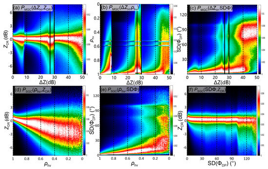
Figure 6.
(a–c) The two-dimensional joint probability density function of PMGC(ΔZH, ZDR), PMGC(ΔZH, ρhv) and PMGC(ΔZH, SD(ΦDP)). The statistical data were collected from the MGC regions between 2016 and 2017 and limited to the thresholds of SNR > 25 dB and pixel altitude < 3.5 km. (d–f) The same as (a–c) but for PSGC(ρhv, ZDR), PSGC(ρhv, SD(ΦDP)) and PSGC(SD(ΦDP), ZDR)) collected from the SGC regions.
ΔZH represents the extent of ground clutter near the radar mainlobe. When the clutter influence was weak, the distribution of ZDR was mainly concentrated between 0 and 1.5 dB, representing the dynamic range of rainfall. As the clutter contamination deteriorated, the probability of the ZDR outliers rapidly increased and the center of the ZDR distribution tended to a negative value. When serious terrain (ΔZH > 50 dB) was observed by the radar mainlobe, the value of ZDR randomly ranged between −8 and 4 dB and the rainfall characteristics totally disappeared. Since three different filtering windows (i.e., rectangular window, Hamming window and Blackman window) were automatically selected by the GMAP scheme according to the extent of ground clutter, the deteriorated trend was divided into three subintervals wherein the ΔZH ranged from 0–8.5, 8.5–30 and 30–50 dB. The monotonically deteriorated trend was reversed at the subinterval junction and the dispersion representing the data quality was partly improved at the beginning of the next interval. For other polarimetric measurements, the contaminated characteristics were similar to those of ZDR. The probability of ρhv < 0.9 and SD(ΦDP) > 10° rapidly increased as the mainlobe contamination deteriorated, significantly differing from the rainfall characteristics.
Owing to the many-to-many correspondence of polarimetric measurements introduced by different filtering windows, ΔZH was more suitable to quantitatively describe the mainlobe clutter. However, the value of ΔZH was often small in the SGC regions and the numerical resolution of ZH (0.5 dB) was insufficient to accurately describe the random dispersions caused by the sidelobe clutters. Considering that the filter under weak clutter influence was the same in the GMAP scheme, a dispersion relationship between the polarimetric measurements was found in the joint probability distributions of PSGC(ρhv, ZDR), PSGC(ρhv, SD(ΦDP)) and PSGC(SD(ΦDP), ZDR) in Figure 6d–f. With the decrease in ρhv and the increase in SD(ΦDP) affected by sidelobe contamination, the dispersion of ZDR rapidly deteriorated and randomly turned to a negative value. Compared with the above two distributions, the trend of ρhv was obviously smoother, which was more suitable to quantify the random errors in the SGC regions.
Based on the above two-dimensional joint probability distributions, the marginal probability functions of PMGC(ZDR|ΔZH), PMGC(ρhv|ΔZH) and PMGC(SDΦ|ΔZH) in Figure 7a–c were used to reveal the differences of data distribution between the pure rain and clutter-contaminated regions. The marginal probability of ZDR in NGC regions was similar to the normal distribution function, where the peak value corresponded to the size-weighted average value of DSD. The function of ρhv and SD(ΦDP) was similar to the semi-normal distribution concentrated at 1 or 0. With the increase of random errors by MGC contamination, the variance in marginal functions exceeded that of rainfall, decreasing the integral result in the fixed rainfall range. This is the reason for the significant difference of the averaged PRA in the MGC, SGC and NGC regions described in Section 3.2. Then, the averaged PRA was decomposed into three independent measurements of ZDR, ρhv and SD(ΦDP), their prior probability of PRA(ZDR), PRA(ρhv) and PRA(SDΦDP) is illustrated in Table 1. As the contaminated levels increase, PRA(ZDR) decreased from 0.97 (pure rain) to 0.71 (ΔZH = 1 dB) and eventually reached only 0.26 (ΔZH = 50 dB). PRA(ρhv) and PRA(SDΦDP) decreased at a faster rate, their values were only 0.07 and 0.01 at a ΔZH value of 50 dB, suggesting that ρhv and ΦDP were more sensitive to clutter influence. For the three subintervals introduced by the GMAP scheme, the most significant deterioration occurred in the subinterval of 0–8.5 dB, where the PRA(ZDR), PRA(ρhv) and PRA(SDΦ) decreased by 0.06, 0.10 and 0.07, respectively, for every 1 dB increase in ΔZH on average. For the dispersion improvement at the subinterval junctions, PRA(ρhv) showed the most obvious change, increasing by 0.48 and 0.22, while little improvement could be found in PRA(SDΦ).
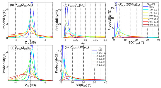
Figure 7.
(a) The marginal probability functions of PMGC(ZDR|ΔZH) calculated using the two-dimensional joint probability functions in Figure 6. (b–e) Same as (a) but for PMGC(ρhv|ΔZH), PMGC(SDΦ|ΔZH), PSGC(ZDR|ρhv) and PSGC(SDΦ|ρhv).

Table 1.
The priori probability of PRA(ZDR), PRA(ρhv) and PRA(SDΦDP) under different levels of clutter contamination.
Figure 7d–e shows the marginal probability functions of PSGC(ZDR|ρhv) and PSGC(SDΦ|ρhv) calculated in the SGC regions. As ρhv decreased from 1.0 to 0.4, the variance of the distribution functions and the negative trend of the mean value gradually changed. On average, the PRA of ZDR and ΦDP decreased by 0.12 and 0.14, respectively, for every 0.1-reduction in ρhv. According to this trend, the prior probability dropped to ~0.5 when ρhv was 0.8 and dropped below 0.2 when ρhv < 0.6. Therefore, the SGC contamination caused by the radar sidelobe could also reach a severe impact similar to that of the MGC contamination.
3.4. Influence of Ground Clutter Contamination under Different Rainfall Intensities
Considering the contaminated measurements come from the fitting results of a Gaussian weather model and the suppression results of a Gaussian clutter model in the GMAP scheme, these restored observations depend on both the spectral information of rainfall and the intensity of ground clutters. Figure 8 illustrates the marginal probability functions under different rainfall intensities, where the threshold of ZH was taken as a simple criterion to classify all pixels into light rain (0–20 dBZ), moderate rain (20–40 dBZ) and heavy rain (40–70 dBZ) [13]. Note that the sampling method was the same as that in Section 3.3 and all pixels with low SNR or ice-phase were excluded.
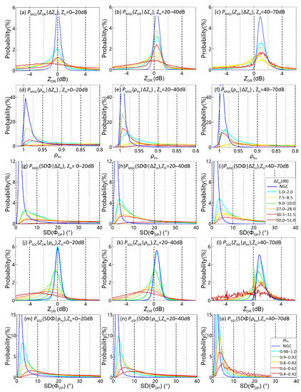
Figure 8.
Marginal probability functions of PMGC(ZDR|ΔZH) in (a) light rain (ZH = 0–20 dBZ), (b) moderate rain (ZH = 20–40 dBZ) and (c) heavy rain (ZH = 40–70 dBZ), where statistical data were collected from the MGC regions between 2016 and 2017 and limited to the thresholds of SNR > 25 dB and pixel altitude < 3.5 km. (d–i) The same as (a–c) but for the marginal probability functions of PMGC(ρhv|ΔZH) and PMGC(SDΦ|ΔZH). (j–o) Marginal probability functions of PSGC(ZDR|ρhv) and PSGC(SDΦ|ρhv) calculated in the SGC regions under light, moderate and heavy rain conditions.
In the NGC regions unaffected by clutter contamination, the marginal distribution functions under different rainfall intensities were similar. Although the DSD variability shifted the mean value of the ZDR functions along the x-axis, the shape and peak values remained unchanged. In the MGC regions representing the mainlobe contamination, the PMGC showed a more deteriorated dispersion in light rain. The prior probability of PRA(ZDR) and PRA(ρhv) calculated in light rain was weaker by 20% to 30% than that in moderate rainfall. A slight difference (~5%) was also found between moderate and heavy rain but it might be related to some hydrometeors in severe storms (e.g., heavy rain and hail) with high dispersion rather than the clutter contamination. As the extent of the mainlobe clutters became more severe in above three subintervals, the concentration of the marginal function substantially decreased, regardless of the rainfall intensity. Therefore, the relative intensity of the rainfall and mainlobe ground clutter determined the data quality of polarimetric measurements. When the rainfall was strong and the clutter was weak, the spectrum information of the meteorological signals was more abundant in the frequency domain for clutter mitigation and data restoring and vice versa.
For the SGC regions in Figure 8j–l, the ZDR distribution under different rainfall intensities was almost the same and it rapidly shifted to negative values with decreasing ρhv. Thus, the influence of sidelobe contamination on ZDR was similar to a random error and unrelated to the precipitation type. The sensitivity of ΦDP measurement to clutter contamination was caused by the differential backscatter phase shift δ under non-Rayleigh scattering. As the rainfall intensified, the decreased δ effect and the increased PRA(ΦDP) demonstrated the well availability of ΦDP in the sidelobe contaminated regions.
4. Impact of Ground Clutter Contamination on Polarimetric Algorithms
4.1. Performance Uncertainty of the Hydrometeor Classification Algorithm Caused by Ground Clutter Contamination
The principle of the HC algorithm is to match the real-time polarimetric observations with preset observational characteristics and the hydrometeor with the highest matching degree is selected as the classification result. Due to the clutter contamination in the MGC and SGC regions, the outliers of polarimetric measurements might not fit the previously established parameter table, thereby, decreasing the algorithm’s stability. Figure 9 shows the horizontal structures and HC results of a squall line observed by the GZ radar on 13 April 2016.
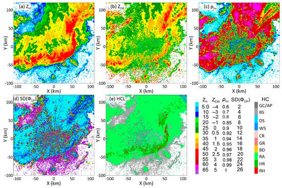
Figure 9.
Horizontal structures of (a) ZH, (b) ZDR, (c) ρhv, (d) SD(ΦDP) after clutter mitigation and (e) hydrometeor classification (HC) results at an elevation angle of 0.5° by the GZ radar at 0606 LST on 13 April 2016.
The bow echo was located in the leading edge (Figure 9a), where the ZH of severe convective storms ranged up to 50–60 dBZ. The stratiform clouds with uniform structures were in the back and the ZH ranged between 30 and 40 dBZ. Obvious clutter features with large SD(ΦDP), small ZDR and ρhv (Figure 9b–d) were consistent with the findings in Section 3. Although the hydrometeors of RA, HR and RH appeared in reasonable positions in the HC result (Figure 9e), more GC/AP and BS that represent non-meteorological echoes were embedded in them. Apparently, the clutter contamination increased the proportion of the non-meteorological echoes and decreased the data consistency.
The proportion of each hydrometeor class in the NGC regions between 2016 and 2017, representing the climate characteristics of GZ radar, was used as the criterion to quantitatively analyze the clutter impact on the HC algorithm. The absolute and relative errors of each class were shown in Figure 10a and the pixel numbers in the MGC, SGC and NGC regions were limited to be approximately equal to guarantee the representativeness of statistical results. Evidently, the frequency of the GC/AP and BS class in the clutter-contaminated pixels was several times than that in normal pixels and the proportion of other hydrometeor classes almost decreased. Histograms reveals that the relative error was related to both the clutter degree and the phase state of the HC class. Due to the severe impact of mainlobe contamination, the changed proportion in the MGC regions was 1.5 to 2 times that in the SGC regions. Similarly, owing to the concentrated polarimetric characteristics of ice-phase hydrometeors, the DS, WS, CR and GR classes showed weaker capabilities of fault tolerance than that of RA class. A phenomenon related to false alarms should be pointed out. The decreased ZDR and ρhv caused by ground clutter were consistent with the membership functions of HR and RH, causing an abnormal increase of the above two classes in the contaminated regions.
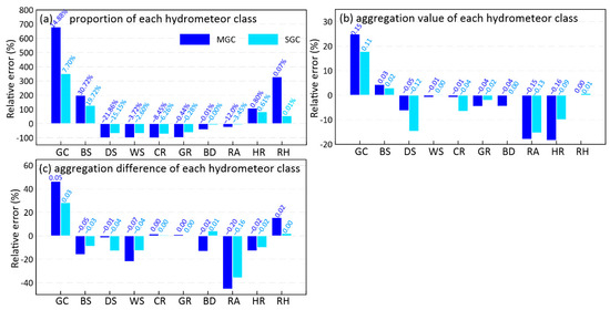
Figure 10.
(a) Comparison of the HC proportion of the clutter-contaminated MGC and SGC regions with that of the pure rain region observed by the GZ radar in 2016 and 2017. The pixels were limited to the loop region between a radius of 40–60 km. The histogram represents the relative error between the clutter-contaminated region and the pure rain region and the absolute error is marked with values above the histogram. (b,c) The same as (a) but for comparison of the maximum aggregation value and the aggregation difference between the maximum and sub-maximum value in the fuzzy logic approach.
For the classification process of each pixel, the maximum aggregation value represents the matching degree between the membership function and the radar measurements, meanwhile the aggregation difference between the maximum and the sub-maximum value represents the discrimination of each membership function. According to the statistics of GZ radar in the NGC regions, the maximum aggregation value ranged between 0.7 and 0.9 and the aggregation difference ranged between 0.15 and 0.45, demonstrating the well-performance of the fuzzy logic approach. When contaminated measurements were taken as the algorithm input, the changed HC proportion was accompanied by performance deterioration of the membership functions. Figure 10b,c shows the absolute and relative errors of the maximum aggregation values and the aggregation differences in the MGC and SGC regions. A significant decrease was found in hydrometeors of RA and HR, corresponding to a negative impact on the matching degree and discrimination. As the proportion of RA and HR changed conversely in Figure 10a, it implies that a part of the RA was misclassified to HR and other hydrometeors due to clutter influence. Unexpectedly, the deteriorated performance between the MGC and SGC regions or the ice-phase and liquid-phase hydrometeors was similar in most membership functions. A reasonable explanation is that strong mainlobe contamination can directly change the classification result, rendering the discussion on the functional performance redundant. Only some weak clutter influences can affect the matching degree and discrimination of the membership functions without changing the final classification result.
In order to deal with the deteriorated performance of the HC algorithm, a feasible method is to discriminate whether the pixel is contaminated through the long-term statistics. The decision tree algorithm may work in the clutter-contaminated region to avoid the uncertain results of the fuzzy logic approach.
4.2. Extra Error of the Quantitative Precipitation Estimation Algorithm Caused by Ground Clutter Contamination
The polarimetric empirical relationships with DSD information have been proved to effectively reduce the rainfall estimation error. But the majority of the polarimetric measurements in the MGC and SGC regions were not performed in the common distribution of pure rain and the extra error caused by clutter contamination should not be ignored. Figure 11 shows the horizontal structures of instantaneous rain rates of a squall line retrieved by the R(ZH) = 0.0196 ZH0.688, R(ZH, ZDR) = 0.0196 ZH0.688 ZDR−3.49, R(KDP) = 44.5 KDP0.782 and R(AH) = 4120 AH1.03. The observation time and elevation angle are the same as those in Figure 9.
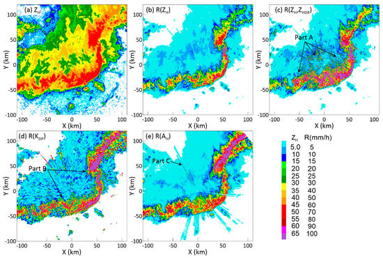
Figure 11.
The same as Figure 9 but for (a) ZH after clutter mitigation, (b) rain rate retrieved from the R(ZH) relation, (c) rain rate retrieved from the R(ZH, ZDR) relation, (d) rain rate retrieved from the R(KDP) relation and (e) rain rate retrieved from the R(AH) relation.
Compared with the classical R(ZH) (Figure 11b), some anomalous characteristics caused by the clutter contamination were found in the polarimetric-retrieved structures. For the rain rate retrieved by the R(ZH, ZDR) relation (Figure 11c), the area of heavy rainfall abnormally extended to the stratiform region (Part A) and coincided with the negative-ZDR region by clutter contamination. This was due to the inverse ratio between the ZDR and the retrieved results in the formula, the smaller ZDR in MGC and SGC regions substantially increased the QPE error. The non-uniform structure of R(KDP) (Figure 11d) was related to the KDP estimation by using the linear regression of the 9/25-points window along the radial. The deficiencies of anomalous fluctuations in stratiform regions and extra errors by long-distance fitting were still difficult to solve, thereby overestimating the light rainfall (Part B). This limitation of KDP can be partially avoided using specific attenuation AH, which was calculated from the total span of ΦDP along the propagation path. Figure 11e illustrates the reasonably results of R(AH) in both the convective and stratiform regions. But when pixels at the start or end of the radial were contaminated by clutters, some outliers still existed in a few radials (Part C).
The correlation coefficient (CC), root-mean-square error (RMSE) and relative error (RE) between the radar-retrieved rainfall and rain gauge measurements were used to quantitatively validate the performance of the R(ZH), R(ZH, ZDR), R(KDP) and R(AH) relations in the MGC, SGC and NGC regions. Considering the huge uncertainty of the estimation accuracy (e.g., rain band evolution, sampling volume difference, etc.), a series of restrictions were adopted in the comparison. Only precipitation cases of large-scale (i.e., 80% gauges in the radar coverage observed rainfall) and long duration (i.e., rainfall lasts more than 5 h) observed by the GZ radar in 2016 and 2017 were counted and the statistical pixels were limited to a loop region 45 to 60 km away from the radar to reduce the extra errors caused by the varying sampling volume.
The scatterplots of the retrieved hourly rainfall versus the gauge measurements in Figure 12 reveal that the estimation errors primarily originate from the performance of empirical relations and the negative influence of ground clutter. For the classical R(ZH) formula, no significant dispersion was found in the MGC, SGC and NGC regions, demonstrating the clutter impact was relatively weak. But all the scatters of the R(ZH) relation exhibited an overall underestimation of ~30% due to the DSD variability. In contrast, the estimation error of the R(ZH, ZDR) formula was significantly improved for the uncontaminated pixels. The RE was reduced to −2.24% with the CC maintained high, almost solving the underestimation of R(ZH) in heavy rainfall. However, the R(ZH, ZDR) relation was very sensitive to the clutter impact, once any pixels were contaminated by clutters, the extra error would be far greater than that of the classical R(ZH) algorithm. Similarly, the uncertainty of the KDP calculation caused an overestimation of R(KDP) in the part of light rain. With the rapid growth of SD(ΦDP) in the contaminated regions, the performance of R(KDP) significantly deteriorated, revealing that inappropriate application introduced more estimation errors. Among the above algorithms, the result of R(AH) exhibited the best stability. The RE of the R(AH) relation was maintained within 4% and few changes of the RMSE and CC were found in the MGC and SGC regions. In fact, no matter the measurements were contaminated by clutters or not, the performance of the R(AH) relation mainly achieved the same of R(ZH, ZDR) in the NGC regions.
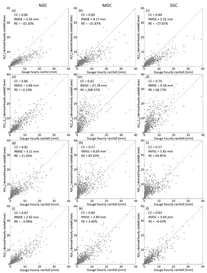
Figure 12.
Scatterplots of retrieved hourly rainfall vs. gauge observations: (a) R(ZH) in the NGC region, (b) R(ZH) in the MGC region, (c) R(ZH) in the SGC region. (d–f), (g–i), (j–l) The same as (a–c) but for the retrieved results of R(ZH, ZDR), R(KDP) and R(AH), respectively. The radar dataset came from 12 long-term rainfall cases with 75 h observations by the GZ radar in 2016 and 2017, the pixels were limited to a loop region ranging from a 45 to 60 km radius. The gauge dataset came from 42 rain gauges in the loop region where number of gauges in the MGC, SGC and NGC regions were approximately equal.
To reduce the extra error caused by clutter contamination, the R(AH) algorithm with high performance and stability should be further promoted. While for the application of other polarimetric algorithms, the accumulated data through long-term statistics is necessary to determine whether it can be used in this pixel.
5. Summary
Through the long-term statistics of eight polarimetric radars in South China, this article analyzed the characteristics and spatiotemporal distribution of ground clutter contamination. This contamination was characterized by the decreased ZDR, ρhv and the increased SD(ΦDP) that simultaneously appeared in the radar mainlobe and sidelobe. The source of these outliers mainly came from the non-Rayleigh scattering between two orthogonal channels and the filter response to different clutter levels. For most radar sites, the proportion of contaminated pixels was much larger than that caused by the beam blockage, resulting in a large-area and long-term anomalies. Whether the polarimetric contamination stemmed from the mainlobe or sidelobe clutter, both could completely deviate meteorological echoes under severe conditions. By comparing the prior probability density functions of contaminated pixels, ΔZH and ρhv were deemed suitable to quantitatively describe the random dispersion.
The ground clutter also exhibited a significant influence on the algorithm stability of the hydrometeor classification and precipitation estimation products. The frequency of non-meteorological echoes increased in the clutter-influenced regions, corresponding to a large reduction in other hydrometeors. The fundamental reason for the uncertainty of classification algorithm came from the deteriorated performance of the fuzzy logic approach, wherein both the matching degree and discrimination of membership functions were reduced. Poor performance was also found in the rainfall estimation algorithm. Even slight sidelobe contamination could easily break the established empirical relations of R(ZH, ZDR) and R(KDP). The extra error was considerably greater than the uncertainty caused by the DSD variability of R(ZH). Only the retrieved results from R(AH) exhibited a relatively balanced performance and stability.
The above results highlighted the negative influence of ground clutter on polarimetric measurements and products. A discrimination mechanism based on long-term statistics is recommended for all polarimetric applications. Considering that an increasing number of polarimetric radar is being deployed in China, more in-depth studies are required.
Author Contributions
Conceptualization, methodology and investigation, C.W. and L.L.; resources, data curation and validation, C.C. and C.Z.; writing—review and editing, G.H. and J.L. All authors have read and agreed to the published version of the manuscript.
Funding
This work was supported by the National Key Research and Development Plan of China (Grant No. 2018YFC1506101 and Grant No. 2018YFC1507401), the Open Research Program of the State Key Laboratory of Severe Weather (Grant No. 2020LASW-B02 and Grant No. 2020LASW-B09).
Institutional Review Board Statement
Not applicable.
Informed Consent Statement
Not applicable.
Data Availability Statement
Data sharing not applicable.
Conflicts of Interest
The authors declare no conflict of interest.
References
- Doviak, R.J.; Zrnic, D.S. Doppler Radar and Weather Observations, 2nd ed.; Dover Publications: New York, NY, USA, 1984; p. 592. [Google Scholar]
- Fabry, F. Radar Meteorology: Principles and Practice, 1st ed.; Cambridge University Press: Cambridge, UK, 2015; p. 86. [Google Scholar]
- Siggia, A.; Passarelli, J.R. Gaussian model adaptive processing (GMAP) for improved ground clutter cancellation and moment calculation. In Proceedings of the Third European Conference on Radar in Meteorology and Hydrology, Visby, Gotland, Sweden, 6–10 September 2004; pp. 67–73. [Google Scholar]
- Hubbert, J.C.; Dixon, M.; Ellis, S.M.; Meymaris, G. Weather radar ground clutter. Part I: Identification, modeling, and simulation. J. Atmos. Ocean. Technol. 2009, 26, 1165–1180. [Google Scholar] [CrossRef]
- Hubbert, J.C.; Dixon, M.; Ellis, S.M. Weather radar ground clutter. Part II: Real-Time identification and filtering. J. Atmos. Ocean. Technol. 2009, 26, 1181–1197. [Google Scholar] [CrossRef]
- Torres, S.M.; Warde, D.A. Ground clutter mitigation for weather radars using the autocorrelation spectral density. J. Atmos. Oceanic Technol. 2014, 31, 2049–2066. [Google Scholar] [CrossRef]
- Li, Y.; Zhang, G.; Doviak, R.J.; Lei, L.; Cao, Q. A new approach to detect ground clutter mixed with weather signals. IEEE Trans. Geosci. Remote Sens. 2013, 51, 2373–2387. [Google Scholar] [CrossRef]
- Golbon-Haghighi, M.-H.; Zhang, G. Detection of ground clutter for dual-polarization weather radar using a novel 3D discri-minant function. J. Atmos. Ocean. Technol. 2019, 36, 1285–1296. [Google Scholar] [CrossRef]
- Junyent, F.; Chandrasekar, V. An examination of precipitation using CSU–CHILL dual-wavelength, dual-polarization radar observations. J. Atmos. Ocean. Technol. 2016, 33, 313–329. [Google Scholar] [CrossRef]
- Gourley, J.J.; Tabary, P.; Chatelet, P. A fuzzy logic algorithm for the separation of precipitating from nonprecipitating echoes using polarimetric radar observations. J. Atmos. Oceanic Technol. 2007, 24, 1439–1451. [Google Scholar] [CrossRef]
- Germann, U.; Galli, G.; Boscacci, M.; Bolliger, M. Radar precipitation measurement in a mountainous region. Q. J. R. Meteorol. Soc. 2006, 132, 1669–1692. [Google Scholar] [CrossRef]
- Gabella, M.; Notarpietro, R. Ground clutter characterization and elimination in mountainous terrain. In Proceedings of the Second European Conference on Radar meteorology, Delft, The Netherlands, 18–22 November 2002; pp. 305–311. [Google Scholar]
- Park, H.; Ryzhkov, A.V.; Zrnic, D.S.; Kim, K.-E. The hydrometeor classification algorithm for the polarimetric WSR-88D: De-scription and application to an MCS. Weather Forecast. 2009, 24, 730–748. [Google Scholar] [CrossRef]
- Elmore, K.L. The NSSL hydrometeor classification algorithm in winter surface precipitation: Evaluation and future development. Weather Forecast. 2011, 26, 756–765. [Google Scholar] [CrossRef]
- Snyder, J.C.; Ryzhkov, A.V. Automated detection of polarimetric tornadic debris signatures using a hydrometeor classification algorithm. J. Appl. Meteor. Climatol. 2015, 54, 1861–1870. [Google Scholar] [CrossRef]
- Lim, S.; Cifelli, R.; Chandrasekar, V.; Matrosov, S.Y. Precipitation Classification and Quantification Using X-Band Du-al-Polarization Weather Radar: Application in the Hydrometeorology Testbed. J. Atmos. Ocean. Technol. 2013, 30, 2108–2120. [Google Scholar] [CrossRef]
- Wang, Y.; Chandrasekar, V. Algorithm for estimation of the specific differential phase. J. Atmos. Oceanic Technol. 2009, 26, 2565–2578. [Google Scholar] [CrossRef]
- Wang, Y.; Zhang, J.; Ryzhkov, A.V.; Tang, L. C-band polarimetric radar QPEs based on specific differential propagation phase for extreme typhoon rainfall. J. Atmos. Oceanic Technol. 2013, 30, 1354–1370. [Google Scholar] [CrossRef]
- Wang, Y.; Cocks, S.; Tang, L.; Ruzhkov, A.; Zhang, P.; Zhang, J.; Howard, K. A prototype quantitative precipitation esti-mation algorithm for operational S-Band polarimetric radar utilizing specific attenuation and specific differential phase. Part I: Algorithm description. J. Hydrometeor. 2019, 20, 985–997. [Google Scholar] [CrossRef]
- Ma, Y.; Chandrasekar, V. A Hierarchical Bayesian Approach for Bias Correction of NEXRAD Dual-Polarization Rainfall Esti-mates: Case Study on Hurricane Irma in Florida. IEEE Geoence Remote Sens. Lett. 2020, 99, 1–5. [Google Scholar]
- Ma, Y.; Chandrasekar, V.; Biswas, S.K. A Bayesian correction approach for improving Dual-frequency Precipitation Radar rainfall rate estimates. J. Meteor. Soc. Jpn. 2020, 98, 511–525. [Google Scholar] [CrossRef]
- Chen, H.; Cifelli, R.; Chandrasekar, V.; Ma, Y. A Flexible Bayesian Approach to Bias Correction of Radar-Derived Precipitation Estimates over Complex Terrain: Model Design and Initial Verification. J. Hydrometeor. 2019, 20, 2367–2382. [Google Scholar] [CrossRef]
- Cifelli, R.; Chandrasekar, V.; Chen, H.; Johnson, L.E. High Resolution Radar Quantitative Precipitation Estimation in the San Francisco Bay Area: Rainfall Monitoring for the Urban Environment. J. Meteorol. Soc. Jpn. 2018, 96A, 141–155. [Google Scholar] [CrossRef]
- Chen, H.; Cifelli, R.; White, A. Improving operational radar rainfall estimates using profiler observations over complex terrain in Northern California. IEEE Trans. Geosci. Remote Sens. 2019, 58, 1821–1832. [Google Scholar] [CrossRef]
- Pulkkinen, S.; Koistinen, J.; Kuitunen, T.; Harri, A.-M. Probabilistic radar-gauge merging by multivariate spatiotemporal tech-niques. J. Hydrol. 2016, 542, 662–678. [Google Scholar] [CrossRef]
- Gou, Y.; Ma, Y.; Chen, H.; Yin, J. Utilization of a C-band polarimetric radar for severe rainfall event analysis in complex terrain over Eastern China. Remote Sens. 2019, 11, 22. [Google Scholar] [CrossRef]
- Chen, H.; Chandrasekar, V. An improved dual-polarization radar rainfall algorithm (DROPS2.0): Application in NASA IFloods field campaign. J. Hydrometeor. 2017, 18, 917–937. [Google Scholar] [CrossRef]
- Pulkkinen, S.; Chandrasekar, V.; Harri, A. Nowcasting of precipitation in the high-resolution Dallas–Fort Worth (DFW) urban radar remote sensing network. IEEE J. Sel. Top. Appl. Earth Obs. Remote Sens. 2018, 11, 2773–2787. [Google Scholar] [CrossRef]
- Pulkkinen, S.; Chandrasekar, V.; Harri, A. Stochastic Spectral Method for Radar-Based Probabilistic Precipitation Nowcasting. J. Atmos. Oceanic Technol. 2019, 36, 971–985. [Google Scholar] [CrossRef]
- Wang, S.D.; Pei, C.; Guo, Z.M.; Shao, N. Evaluations on chinese next generation radars coverage and terrain blockage based on SRTM data. Climatic. Environ. Res. 2011, 16, 459–468. (In Chinese) [Google Scholar]
- Shi, B.L.; Wang, H.Y.; Liu, L.P. Coverage capacity of hail detection for Yunnan Doppler weather radar network. J. Appl. Meteor. Sci. 2018, 29, 270–281. (In Chinese) [Google Scholar]
- Wang, H.Y.; Wang, G.L.; Liu, L.P. Climatological beam propagation conditions for China’s weather radar network. J. Appl. Meteor. 2017, 57, 3–14. [Google Scholar] [CrossRef]
- Ma, Y.; Tang, G.; Long, D.; Yong, B.; Zhong, L.; Wan, W.; Hong, Y. Similarity and error intercomparison of the GPM and its predecessor-TRMM multisatellite precipitation analysis using the best available hourly gauge network over the Tibetan Plateau. Remote Sens. 2016, 8, 569. [Google Scholar] [CrossRef]
- Ma, Y.; Yang, Y.; Han, Z.; Tang, G.; Maguire, L.; Chu, Z.; Hong, Y. Comprehensive evaluation of Ensemble Multi-Satellite Precipitation Dataset using the Dynamic Bayesian Model Averaging scheme over the Tibetan plateau. J. Hydrol. 2018, 556, 634–644. [Google Scholar] [CrossRef]
- Ma, Y.; Hong, Y.; Chen, Y.; Yang, Y.; Tang, G.; Yao, Y.; Long, D.; Li, C.; Han, Z.; Liu, R. Performance of optimally merged multisatellite precipitation products using the dynamic Bayesian model averaging scheme over the Tibetan Plateau. J. Geophys. Res. Atmos. 2018, 123, 814–834. [Google Scholar] [CrossRef]
- Ma, Y.; Lu, M.; Chen, H.; Pan, M.; Hong, Y. Atmospheric moisture transport versus precipitation across the Tibetan Plateau: A mini-review and current challenges. Atmos. Res. 2018, 209, 50–58. [Google Scholar] [CrossRef]
- Chen, H.; Chandrasekar, V.; Tan, H.; Cifelli, R. Rainfall Estimation from Ground Radar and TRMM Precipitation Radar Using Hybrid Deep Neural Networks. Geophys. Res. Lett. 2019, 46, 10669–10678. [Google Scholar] [CrossRef]
- Chen, H.; Chandrasekar, V.; Cifelli, R.; Xie, P. A machine learning system for precipitation estimation using satellite and ground radar network observations. IEEE Trans. Geosci. Remote Sens. 2020, 58, 982–994. [Google Scholar] [CrossRef]
- Luo, Y.; Zhang, R.; Wan, Q.; Wang, B.; Wong, W.K.; Hu, Z.; Jou, B.J.; Lin, Y.; Johnson, R.H.; Chang, C.P.; et al. The Southern China Monsoon Rainfall Experiment (SCMREX). Bull. Am. Meteorol. Soc. 2017, 98, 999–1013. [Google Scholar] [CrossRef]
- Seliga, T.A.; Bringi, V.N. Potential use of radar differential reflectivity measurements at orthogonal polarizations for measuring precipitation. J. Appl. Meteorol. 1976, 15, 69–76. [Google Scholar] [CrossRef]
- Testud, J.; Bouar, E.L.; Obligis, E.; Ali-Mehenni, M. The rain profiling algorithm applied to polarimetric weather radar. J. Atmos. Oceanic Technol. 2000, 17, 332–356. [Google Scholar] [CrossRef]
- Giangrande, S.E.; Ryzhkov, A.V. Estimation of rainfall based on the results of polarimetric echo classification. J. Appl. Meteorol. Climatol. 2008, 47, 2445–2462. [Google Scholar] [CrossRef]
- Chen, H.; Chandrasekar, V. Estimation of light rainfall using Ku-band dual-polarization radar. IEEE Trans. Geosci. Remote Sens. 2015, 53, 5197–5208. [Google Scholar] [CrossRef]
- Cocks, S.; Wang, Y.; Tang, L.; Ryzhkov, A.; Zhang, P.; Zhang, J.; Howard, K. A prototype quantitative precipitation estimation algorithm for operational S-band polarimetric radar utilizing specific attenuation and specific differential phase: Part II–Case study analysis and performance verification. J. Hydrometeorol. 2019, 20, 999–1014. [Google Scholar] [CrossRef]


Publisher’s Note: MDPI stays neutral with regard to jurisdictional claims in published maps and institutional affiliations. |
© 2021 by the authors. Licensee MDPI, Basel, Switzerland. This article is an open access article distributed under the terms and conditions of the Creative Commons Attribution (CC BY) license (http://creativecommons.org/licenses/by/4.0/).