Abstract
Satellites are capable of observing precipitation over large areas and are particularly suitable for estimating precipitation in high mountains and poorly gauged regions. However, the coarse resolution and relatively low accuracy of satellites limit their applications. In this study, a downscaling scheme was developed to obtain precipitation estimates with high resolution and high accuracy in the Heihe watershed. Shannon’s entropy, together with a semi-variogram, was applied to establish the optimal precipitation station network. A combination of the random forest (RF) method and the residual correction approach with the established rain gauge network was applied to downscale monthly precipitation products from Integrated Multi-satellitE Retrievals for Global Precipitation Measurement (IMERG). The results indicated that the RF model showed little improvement in the accuracy of IMERG-based precipitation downscaling. Including residual modification could improve the results of the RF model. The mean absolute error (MAE) and root mean square error (RMSE) values decreased by 19% and 21%, respectively, after residual corrections were added to the RF approach. Moreover, we found that enough rain gauge records are necessary for and remain an important component of tuning model performance. The application of more rain gauges improves the performance of the combined RF and residual modification methods, with the MAE and RMSE values reduced by 8% and 9%, respectively. Residual correction, together with enough precipitation stations, can effectively enhance the quality of the precipitation patterns and magnitudes obtained in the RF downscaling process. The proposed downscaling scheme is an effective tool for increasing the accuracy and spatial resolution of precipitation fields in the Heihe watershed.
1. Introduction
Precipitation is a primary variable associated with earth science, hydrology, climatology, and agriculture [1,2,3,4,5]. The spatial distribution of precipitation is a necessary input for hydrological and ecological models. Accurate and reliable precipitation estimates are crucial for understanding the hydrologic cycle, managing water resources, evaluating hydrological impacts on human life, and forecasting climate trends and variability [6,7,8].
Various approaches have been proposed for estimating distributions of precipitation over the last few decades. These methods are based on mathematical and physical principles determined by using rain gauges, weather radar, satellite sensors, and numerical models. The interpolation method is a common approach used to generate spatial precipitation fields. However, the accuracy of interpolation-based precipitation estimates is significantly dependent on the station network and the degree of the spatial heterogeneity of precipitation [9,10]. It is difficult to gain accurate spatial information on precipitation based on data from stations with sparse coverage and in areas where the spatial heterogeneity of precipitation is high, especially mountainous areas [11]. Numerical models can provide spatial precipitation estimates with physical bases but require large computational resources and have large uncertainties associated with parameters [12,13]. Satellite sensors can detect precipitation information globally and can be applied to high mountains and deserts, but satellite data poorly represent variability in local areas and complex topographical regions due to their low resolutions and deficiencies in retrieval algorithms [14,15,16].
A growing number of multi-sensor blended precipitation products have emerged during the past thirty years. Some previous works focused on comparisons of different remote sensing products at national or regional scales [17,18,19,20]. The Global Precipitation Measurement (GPM) Core Observatory was launched in 2014 to extend the Tropical Rainfall Measuring Mission (TRMM). The Integrated Multi-satellitE Retrievals for GPM (IMERG) provides a new generation of satellite precipitation products that have been widely applied in many fields [21]. Studies have found that the IMERG precipitation products show better performances than other satellite precipitation measurements and reanalysis datasets, such as the TRMM3B42 and ERA-Interim products [22,23,24]. IMERG provides precipitation estimates every 30 min with a spatial resolution of 0.1° depending on the sensors in the TRMM and GPM eras. However, IMERG precipitation products have relatively coarse spatial resolutions that are not sufficiently fine to capture spatial variations in precipitation in complex local landscapes.
To overcome the inherent limitations of IMERG products in fine-scale applications, downscaling techniques are often required to translate precipitation products from a coarse scale to a regional or catchment scale. Dynamical and statistical downscaling methods are two fundamental downscaling techniques. Compared to the dynamical downscaling procedure, statistical downscaling is relatively computationally efficient and aims to establish the statistical relationships between the predictands and predictors of local and large-scale variables [7,25]. Several statistical downscaling approaches have been implemented to derive precipitation fields with fine resolutions, such as geographic weighted regression (GWR), random forest (RF), and artificial neural networks (ANNs) [26,27,28]. Among these methods, RF is recognized for being accurate and able to deal with small sizes and high-dimensional feature spaces [29,30]. Despite the improvements in the spatio-temporal representation of precipitation obtained by these methods, many studies only downscale the satellite products either with the existing limited meteorological observations or without considering the station values [25,26,27,28,29,30,31]. Observations from rain gauges are ideally used as necessary inputs for downscaling. For complex topographical regions and high mountains, however, the density and spacing of the rain gauges restrict the accuracy of the downscaling methods. Studies have also shown that the marginal effect of introducing auxiliary variables is more obvious for low-density station networks than for high-density station networks [32]. In addition, the establishment of more rain gauges requires considerable financial and technological investments for operational and maintenance costs.
The goal of this paper is to provide monthly precipitation estimates with a high spatial resolution in the Heihe watershed in China by downscaling IMERG products. To obtain reliable precipitation estimates, a method composed of Shannon’s entropy and a semi-variogram was used to first establish virtual rain gauges based on the existing meteorological stations and local topographical features. The values of the virtual rainfall gauges were obtained by applying the Weather Research and Forecasting Model (WRF). The RF method was then applied to downscale the IMERG precipitation data from 0.1° to 0.01°, combined with virtual and existing rainfall gauges and auxiliary information. The downscaling scheme was expected to reduce the spatial resolution of IMERG data and effectively enhance the quality of precipitation patterns and magnitudes.
2. Study Area and Data
The Heihe watershed is the second-largest inland river basin in China and falls in the category of an arid region with a total area of approximately 140,000 km2 (Figure 1). The river originates in the Qilian Mountains, flows through an irrigated agricultural area, continues northward, and finally joins two lakes in the desert. The elevation ranges from 872 m in the north to more than 5000 m in the south above the sea level, with high spatial heterogeneity in altitude. The watershed is divided into three segments: the upper, middle, and lower reaches, with high mountains and plateaus located in the southern area, occupying 33.6% of the whole watershed, and oases and deserts distributed in the middle and low reaches, accounting for 8.9% and 57.5% of the study area, respectively. The climate is mainly controlled by westerlies throughout the year. The precipitation in the watershed shows strong spatial heterogeneity, with an annual mean precipitation varying from less than 50 mm in the low reach to more than 550 mm in the upper reach, and more than 60% of the annual precipitation occurs in the summer months, from May to September [31,33]. The Heihe watershed is poorly gauged, with two stations located in the lower reach, seven stations located in the middle reach and four stations distributed in the upper reach. Eleven stations are located in areas below 2800 m in elevation, two stations are located between elevations of 2800 and 3500 m, and there are no stations found above 3500 m (Table 1).
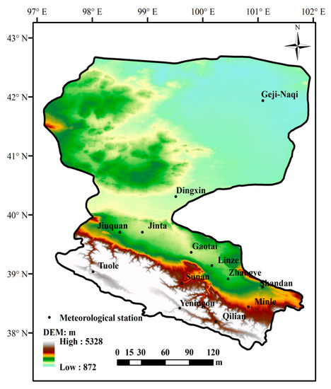
Figure 1.
Heihe watershed boundary and meteorological stations.

Table 1.
Geographical information and precipitation observations of the 13 meteorological stations available for public use.
The GMP IMERG product supersedes the TRMM product as the next-generation precipitation dataset developed with GPM data through the assimilation of information from multiple MW/IR sensors together with ground observations. The GPM provides global precipitation estimates with a spatial resolution of 0.1° and a relatively high temporal resolution of 30 min within the range of 60 °N–60 °S [24,34,35]. In the new version of IMERG, an improved algorithm is applied to produce precipitation estimates covering the period from 2000 to the present with a high accuracy. In this research, monthly IMERG V06 data (0.1°, 2000—present) were downloaded from NASA’s data repository [36].
In addition to precipitation itself, other auxiliary predictors are commonly considered during the downscaling process, including elevation, slope, aspect, relief, distance to the sea, and the vegetation index [7,25,37,38]. Elevation data (DEM) were extracted from https://gisgeography.com/free-global -dem-data-sources/, released by the United States government. Slope, aspect and relief data were derived from the DEM using ArcGIS software. The normalized difference vegetation index (NDVI), downloaded from https://modis.gsfc.nasa.gov/, was used as an auxiliary variable in precipitation downscaling [39].
3. Methods
3.1. Designing a Rain Gauge Network Using Shannon’s Entropy
To obtain reliable precipitation estimations, a dense rain gauge network is necessary. The main purpose of rain gauge network design is to determine the number of stations and their locations to yield the maximum precipitation information and the associated variations. Certain rain gauge density levels have been recommended for different types of landforms by the World Meteorological Organization [40]; for example, 25 km2 per station is needed in mountainous areas with heterogeneous precipitation.
We first determined several candidate locations in areas with no meteorological stations, especially in areas of high altitudes, topographically complex regions, no man’s land, and areas that are poorly gauged, according to the guidelines of the WMO by using ArcGIS. Shannon’s entropy, together with a semi-variogram, was applied to design the optimal rain gauge network.
Entropy is a measure of the information content of events [41] and can be expressed as follows:
where is the probability of the event . For precipitation, measures the average amount of precipitation. The overlapping information could exist in two rain gauge stations. The joint entropy of precipitation from two rain gauges is defined as follows,
Equation (2) defines the uncertainty of the marginal information from two stations, and . Conditional entropy can be used to find the gauge with the lowest reduction in uncertainty or trans-information.
Compute the entropy of every candidate rain gauge in the Heihe watershed and find the rain gauge with the highest uncertainty,
Find the second most important rain gauge, , that has the least common information with the first rain gauge, , by using the following equation,
Calculate the conditional entropy of these gauges with respect to all other rain gauges () and find the site with the minimum reduction in uncertainty,
is the third most important rain gauge. Repeat the procedure that the th important rain gauge satisfies,
The monthly precipitation amounts of the sites can be calculated by using the WRF model, which was initialized by the European Centre for Medium-range Weather Forecasts (ECMWF) global atmospheric reanalysis (ERA-Interim). Lastly, the number of virtual rain gauges can be determined based on the existing meteorological stations in the watershed area by comparing the semi-variograms of the two datasets.
3.2. Random Forest
The RF is a supervised learning algorithm that is applicable to classifications and regressions [42]. In practical applications, the RF-based downscaling method is rather easy to handle with few parameters and is capable of efficiently establishing nonlinear relationships between precipitation and some covariates across heterogeneous landscapes [38,43]. The RF fits a number of regression trees using a subset of the given data and averages the results of all trees to determine the final outputs to improve the model accuracy and reduce overfitting. The equation of the RF can be outlined as follows,
Each tree, , is independently grown to its maximum size from the bootstrap sample that contains two-thirds of the grid cells from the training dataset without any pruning. splits into different branches by minimizing a cost function, that is, the sum of squares error, between the precipitation values and the predictors. An important feature of the RF is that the trees were trained on random subsets of the data, thus generating different precipitation estimates [44].
Regarding the selection of the proper predictors in the RF downscaling method, the coarse-resolution precipitation values in the central and adjacent grid cells are probably the most important predictors [7]. Atmospheric predictors are included to provide temporal information about the downscaled precipitation values. Topographic covariates, such as elevation and slope, are also important here due to the orographic dependence of precipitation, especially in the upper reaches of the watershed. Topographic data are considered here to maintain the spatial pattern of the downscaled precipitation values. NDVI, latitude and longitude are also included because they contain land—atmosphere coupling, geographical and seasonality information.
By establishing the rain gauge network, the IMERG products can be downscaled using the RF combined with covariates. Since regression methods usually cannot quantify the total variation in a given precipitation pattern, some researchers have adopted a residual correction. Studies have shown that the application of residuals of a regression method could produce better predictions than those obtained using only the regression method [31,45,46,47,48,49]. To yield the final results, we also added the modified residuals back to the RF results by using kriging combined with the station values. The weights used in the kriging method were based on the Gaussian semi-variogram model of spatial correlation. The downscaling scheme is presented in Figure 2.
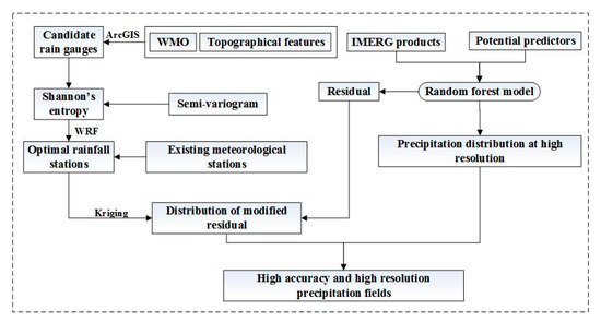
Figure 2.
Illustration of the downscaling scheme.
The accuracy of the downscaling results was assessed by cross-validation of both the existing meteorological stations and the virtual rain gauges. In this approach, precipitation is estimated at a given gauge location using all observations except the one used in the downscaling process [32]. Mean absolute error (MAE) and root mean square error (RMSE) are two common metrics used to measure overall accuracy and reflect extreme outliers, respectively, and were used to compare the different methods in this study. Their equations are given as follows:
where is the true value at the kth location and is the estimated value.
4. Results
By combining Shannon’s entropy with the semi-variogram, the optimal virtual rain gauge network was established (Figure 3), and the monthly precipitation at each gauge was obtained by using WRF. According to the station values of the mean annual precipitation over the past thirty years, a Gaussian semi-variogram model was used and this model was once again applied to fit the relation of the entropy and the optimal stations combination. Finally, fifteen rain gauge stations were selected in this study. The parameterized physical processes in WRF include the Kessler scheme for microphysics, the Mellor Yamada Janjic (MYJ) scheme for the planetary boundary layer, the Monin–Obukhov surface-layer scheme, the rapid radiative transfer model longwave radiation scheme, the Dudhia shortwave radiation scheme, the Kain–Fritsch cumulus scheme, the Noah scheme for the land surface model and the model default terrain information [33]. The locations and estimated monthly precipitation amounts of the 15 virtual rain gauges are listed in Table 2.
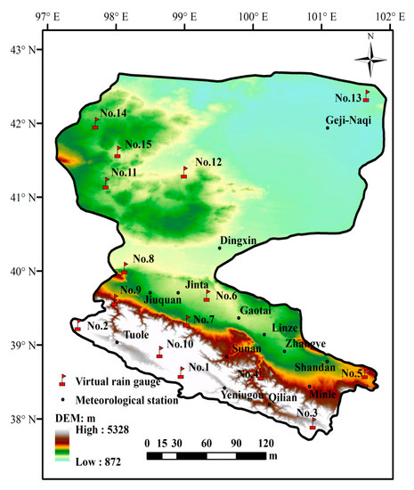
Figure 3.
Optimal rainfall network in the Heihe watershed.
Table 2.
Information on the established virtual rain gauges.
An RF-based downscaling scheme was used to estimate monthly precipitation in the Heihe watershed. First, the impact of adding the residuals back into the RF results was investigated. Next, the performance of the established rain gauge network was evaluated vs. using the only 13 existing meteorological stations. Here, we only present results for July and December 2018 for the two examples. Figure 4 shows the spatial patterns of the GPM IMERG V06B satellite precipitation product and three downscaling results using the RF, the RF plus a residual correction using the 13 meteorological stations (RF_Kri13), and the RF plus a residual correction using a total of 28 stations (RF_Kri28) in July. The IMERG product at 0.1° exhibited a localized pattern with heavy precipitation upstream and a few areas of large precipitation surrounded by low precipitation in the middle and lower reaches. Except for in the northwest region of the watershed, the original IMERG-based precipitation values tended to overestimate precipitation in most parts of the region. The maximum precipitation value obtained from the IMERG product was located in the southeast region of the watershed with a value of 223.1 mm, while the smallest value occurred in the northwest part with a value of 21.8 mm. The downscaled precipitation captured the pattern but large differences existed among some local areas. The residual correction process modified the precipitation amounts, especially in the lower reach (Figure 4c,d). This indicated that the residual correction had a positive effect on the RF-based downscaling method. Compared to the station values, the RF_Kri28 method showed superior performance compared to the RF_Kri13 method. Different spatial patterns were observed in Figure 4c,d, especially in some locations in the middle and lower reaches of the watershed. The virtual rain stations ensured the accuracy of the final precipitation fields, and this improvement was more obvious in the northwest region of the watershed. Furthermore, the scatter correlation plot for the observed and the downscaling results in July (Figure 5) also suggested that RF_Kri28 estimated the precipitation amount quite reliably. The overestimations of IMERG were observed for most of the stations. The results of the RF method had not been significantly improved compared with the original IMERG products. The methods based on residual correction performed better than the RF method, and RF_Kri28 with more station values yielded the best results.
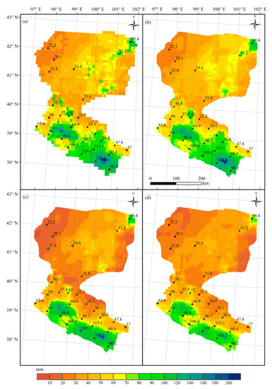
Figure 4.
Integrated Multi-satellitE Retrievals for GPM (IMERG) precipitation at an original resolution of 0.01° and downscaling results in July from (a) the IMERG product; (b) the random forest (RF); (c) the RF_Kri13 method; and (d) the RF_Kri28 method.
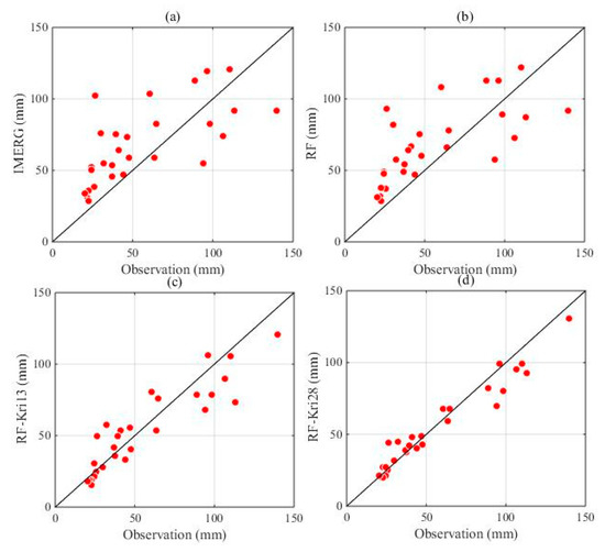
Figure 5.
Observed and downscaled precipitation in July from (a) IMERG product; (b) the RF; (c) the RF_Kri13 method; and (d) the RF_Kri28 method.
The performances of the methods in December are displayed in Figure 6. The IMERG product seemed to underestimate the precipitation in almost the whole watershed compared to the values obtained from the stations. There was no rain in most of the Heihe watershed according to the IMERG product. The RF-based downscaling method (Figure 6b) modified some local details by introducing auxiliary information. The residual correction methods applied after the RF seemed to yield improved precipitation fields. We can see that the RF_Kri28 method performed better than the RF_Kri13 method at 28 gauge locations (Figure 6c,d). The RF_Kri28 method provided more reliable estimates, especially for gauge-sparse areas. In the Heihe watershed, the downscaling method conducted with enough stations performed better than the RF. Clearly, gauge density is an important factor in determining the accuracy of different methods. Figure 7 illustrates the relationship between the gauge values and the downscaled precipitation datasets. Underestimations were both observed for IMERG and the RF method, and to some degree the residual correction process reduced these biases. RF_Kri28 had shown the best agreement with gauge observations (Figure 7d).
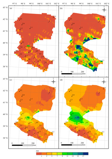
Figure 6.
IMERG precipitation at an original resolution of 0.01° and downscaling results in December from (a) IMERG product; (b) the RF; (c) the RF_Kri13 method; and (d) the RF_Kri28 method.
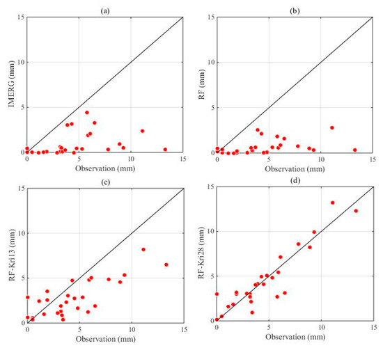
Figure 7.
Observed and downscaled precipitation in December from (a) IMERG product; (b) the RF; (c) the RF_Kri13 method; and (d) the RF_Kri28 method.
The errors presented in Table 3 demonstrate that although the RF approach can provide a precipitation map with a fine resolution, there are limits to the accuracy of the results. In summer months, such as May, July, August and September, the values of MAE and RMSE are slightly larger than those obtained using the IMERG product, possibly due to the lack of other important covariates in the downscaling process, which will be investigated in the future. The application of residuals reduced the values of MAE and RMSE with respect to the RF results. The errors in summer months (from May to September) improved notably, with the mean value of MAE decreasing by 19%, and that of RMSE decreasing by 22%. For the twelve months, the mean values of MAE and RMSE decreased by 15% and 16%, respectively. Residual correction provided obvious reductions in the MAE and RMSE values. The introduction of virtual rain gauges further improved the accuracy of the downscaling fields. For the RF_Kri28 method, the mean values of MAE and RMSE for the twelve months decreased by 8% and 9%, respectively, compared with those obtained in the RF_Kri13 method.
Table 3.
Values of MAE and RMSE for the downscaling results by applying a cross validation technique.
We also compared the downscaled results with the values obtained from the meteorological stations by applying a cross-validation process. Figure 8 displays the area mean absolute bias values of the RF, RF_Kri13, and RF_Kri28 methods for different months over the whole watershed. Compared to those obtained using the RF, significant decreases in the errors can be observed, especially in summer months (from May to September). The RF_Kri28 method achieved better performance than the other methods. The residual correction combined with the application of virtual rain gauges ensured the accuracy of the final precipitation fields.
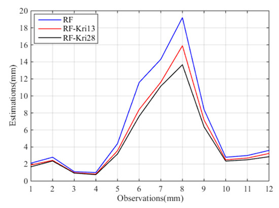
Figure 8.
Mean absolute biases obtained for different downscaling methods.
5. Discussion
Satellite-based precipitation estimates can provide precipitation information with wide spatial coverage, particularly over complex mountainous terrain and sparsely gauged regions. Precipitation data with high accuracy and high spatial resolution play significant roles in forcing local and global climate models and hydrological and ecological models. Studies have shown that the performance of IMERG products is better than those of some other satellite-based precipitation datasets [25,50]. However, in some basins and localized areas, the IMERG products are still too coarse to be applied. Integrating station observations with a single satellite-based precipitation product is a common approach for obtaining high spatial resolution precipitation. Studies have indicated that the use of residual correction methods that use station values can generate better precipitation estimates than regression-based downscaling methods can alone [31,51]. Although scholars have performed much research on the downscaling of satellite products by using geographical and topographical variables and station observations, most of these studies depended on the limited number of existing stations, and the accuracy of the downscaled precipitation products was not significantly improved, especially over high mountainous areas with poor gauged networks.
The main goal of this study was to obtain precipitation estimates with high accuracy and high spatial resolution in a watershed with highly heterogeneous landforms by proposing a downscaling-integration scheme. As denoted, station networks are of primary importance for the accuracy of precipitation estimations [52,53]. A combination of the RF method and the correcting of residuals by using an optimal rain gauge network was thus developed in this study. The optimal station network was designed by using Shannon’s entropy and semi-variograms since entropy can detect the uncertainty information contained in a variable and semi-variograms can be used to determine the number of stations. The precipitation values at the established stations were simulated by using WRF based on the research by Pan [33]. Based on the 13 existing stations and the 15 established virtual rain gauges as well as some covariates, the final downscaling results were obtained by using the RF.
We investigated the performance of the IMERG products in the Heihe watershed. The results in Figure 4, Figure 5, Figure 6 and Figure 7 show that for the original IMERG precipitation datasets, overestimations were observed in almost the whole watershed in July, while underestimations were found in the whole watershed in December, indicating the IMERG products may overestimate precipitation in summer months and underestimate precipitation in winter months. The RF-downscaled precipitation estimates showed similar spatial patterns with those of the IMERG products in July and showed a different but detailed pattern in December (Figure 4b or Figure 6b). However, the accuracy of the RF method was not satisfactory according to the cross-validation process (Table 2), which may be due to the selection of covariates. More predictors will be investigated in future research. The accuracy was obviously improved by applying the residual correction. This finding was consistent with some previous studies that also found that residual modification played a critical role in regression-based estimation methods [25,54,55,56]. The accuracy improved by 19% and 21% according to the MAE and RMSE values, respectively, in this research. We then verified whether the accuracy of the downscaling model could be improved with consideration of virtual rain gauges. The results in Figure 4, Figure 5, Figure 6 and Figure 7 show that additional station values further improved the accuracy of the downscaling results. In terms of the MAE and RMSE values, the errors were reduced by 8% and 9%, respectively, compared to those obtained using observations from the 13 existing stations, and decreased by 22% and 23%, respectively, compared with those obtained via the RF-based downscaling results. This indicated that enough stations were necessary for the downscaling process.
In addition, the statistical results shown in Table 2 and the plots in Figure 8 also indicated that the proposed approach was superior to the other methods. This improvement was attributed to the combined effects of the residual correction and the optimal rain gauge network. However, the established rain gauge network in this study was based on the mean annual precipitation over the past thirty years. Improved results could be obtained by designing the station network in terms of the characteristics of the monthly precipitation. Furthermore, the downscaling scheme would be optimized further by considering more covariates and by adjusting the parameters to make the model more suitable for our study.
6. Conclusions
In this study, a downscaling-integration scheme was developed to generate improved high-accuracy and high-resolution monthly precipitation fields in the Heihe watershed. Shannon’s entropy combined with a semi-variogram was first applied to establish the optimal rain gauge network in the study region. The monthly precipitation amounts at the candidate rain gauges were obtained by using WRF with some suitable localized parameters. Then, the RF was applied to downscale the IMERG precipitation products from a resolution of 0.1° to 0.01° by considering some auxiliary variables, including elevation, slope, aspect, relief, distance to the sea, and the vegetation index, coarse-resolution precipitation values in the central grid cell, and coarse resolution precipitation values at adjacent grid cells. The residuals of the RF results were modified by using the station values from the optimal rain gauge network. The final precipitation estimates were obtained by applying the residual correction to the results of the RF downscaling.
The method was carried out over twelve months in 2018. The performance of the downscaling results based on the RF, RF plus a residual correction using existing 13 stations (RF_Kri13), and RF plus a residual correction using 28 optimal rain gauges (RF_Kri28) were assessed by a cross validation analysis. Studies showed that the original IMERG precipitation products tend to overestimate precipitation in most parts of the watershed in July, and tend to underestimate precipitation in December. The RF approach enhanced the spatial resolution of the precipitation fields without a significant increase in accuracy. A comparison with the station values showed that the precipitation estimates at a high resolution of 0.01° obtained based on the RF_Kri13 and RF_Kri28 methods were better than those obtained from the original IMERG and RF method; the MAE and RMSE values decreased by 19% and 22%, respectively, indicating that the residual correction was beneficial for the RF-based downscaling method. The RF_Kri28 method generated better precipitation estimates than did the RF_Kri13 method, with the values of MAE and RMSE decreasing by 8% and 9%, respectively, demonstrating that the use of a dense rain gauge network further improved the accuracy of the precipitation estimates. The improvement of the final precipitation fields resulted from the combination of the methods of residual correction and the virtual rain gauge establishment.
The benefit of this approach is evident, especially over regions with sparse gauge networks. The downscaling scheme used in this study can be performed for arbitrary target domains, especially in complex mountainous areas and poorly gauged and ungauged basins. In addition, the method used in this study to select optimum precipitation sites can be utilized in developing a particular meteorological station network. It was shown that the presented downscaling scheme is capable of satisfactorily downscaling monthly precipitation fields in the Heihe watershed. Further, investigations may be conducted on a daily time scale with other predictors in the RF downscaling process, such as atmospheric circulation factors.
Funding
This research was funded by the National Natural Science Foundation of China, grant number 42071374 and the Program of Frontier Sciences of Chinese Academy of Sciences, grant number ZDBS-LY-DQC005.
Institutional Review Board Statement
Not applicable.
Informed Consent Statement
Not applicable.
Data Availability Statement
The data are not publicly available due to the confidentiality of the research projects.
Conflicts of Interest
The authors declare no conflict of interest.
References
- Langella, G.; Basile, A.; Bonfante, A.; Terribile, F. High-resolution space–time rainfall analysis using integrated ANN inference systems. J. Hydrol. 2010, 387, 328–342. [Google Scholar] [CrossRef]
- Bruni, G.; Reinoso, R.; van de Giesen, N.C.; Clemens, F.H.L.R.; ten Veldhuis, J.A.E. On the sensitivity of urban hydrodynamic modeling to rainfall spatial and temporal resolution. Hydrol. Earth Syst. Sci. 2015, 19, 691–709. [Google Scholar] [CrossRef]
- Paul, P.K.; Kumari, N.; Panigrahi, N.; Mishra, A.; Singh, R. Implementation of cell-to-cell routing scheme in a large scale conceptual hydrological model. Environ. Modell Softw. 2018, 101, 23–33. [Google Scholar] [CrossRef]
- Piccolroaz, S.; Healey, N.C.; Lenters, J.D.; Schladow, S.G.; Hook, S.J.; Sahoo, G.B.; Toffolon, M. On the predictability of lake surface temperature using air temperature in a changing climate: A case study for Lake Tahoe (U.S.A.). Limnol. Oceanorg. 2018, 63, 243–261. [Google Scholar] [CrossRef]
- Rousta, I.; Olafsson, H.; Moniruaaaman, M.; Zhang, H.; Liou, Y.-A.; Mushore, T.; Mushore, T.D.; Gupta, A. Impacts of drought on Vegetation assessed by vegetation indices and meteorological factors in Afghanistan. Remote Sens. 2020, 12, 2344. [Google Scholar] [CrossRef]
- Singh, R.; Ranjan, K.; Verma, H. Satellite imaging and surveillance of infectious diseases. J. Trop. Dis. 2015, S1-004, 1–6. [Google Scholar] [CrossRef]
- He, X.Y.; Chaney, M.; Schleiss, M.; Sheffield, J. Spatial downscaling of precipitation using adaptable random forests. Water Resour. Res. 2016, 52, 8217–8237. [Google Scholar] [CrossRef]
- Solakian, J.; Maggioni, V.; Godrej, A. Investigating the error propagation from satellite-based input precipitation to output water quality indicators simulated by a hydrologic model. Remote Sens. 2020, 12, 3728. [Google Scholar] [CrossRef]
- Hijmans, R.J.; Cameron, S.E.; Parra, J.L.; Jones, P.G.; Jarvis, A. Very high resolution interpolated climate surfaces for global land areas. Int. J. Climatol. 2005, 25, 1965–1978. [Google Scholar] [CrossRef]
- Rasmussen, R.M.; Baker, B.; Kochendorfer, J.; Meyers, T.; Landolt, S.; Fischer, A.P.; Black, J.; Thériault, J.M.; Kucera, P.; Gochis, D.; et al. How well are we measuring snow: The NOAA/FAA/NCAR winter precipitation test bed. B. Am. Meteorol. Soc. 2012, 93, 811–829. [Google Scholar] [CrossRef]
- Martens, B.; Cabus, P.; Jongh, I.; Verhoest, N.E.C. Merging weather radar observations with ground-based measurements of rainfall using an adaptive multiquadric surface fitting algorithm. J. Hydrol. 2013, 500, 84–96. [Google Scholar] [CrossRef]
- Kidd, C.; Dawkins, E.; Huffman, G. Comparison of precipitation derived from the ECMWF operational forecast model and satellite precipitation datasets. J. Hydrol. 2013, 14, 1463–1482. [Google Scholar] [CrossRef]
- Zhang, X.; Anagnostou, E.N.; Vergara, H. Hydrologic evaluation of NWP-adjusted CMORPH estimates of hurricane-induced precipitation in the Southern Appalachians. J. Hydrol. 2016, 17, 1087–1099. [Google Scholar] [CrossRef]
- Zheng, D.; Bastiaanssen, W.G.M. First results from version 7 TRMM 3B43 precipitation product in combination with a new downscaling–calibration procedure. Remote Sens. Environ. 2013, 131, 1–13. [Google Scholar]
- Adhikary, S.K.; Yilmaz, A.G.; Muttil, N. Optimal design of rain gauge network in the Middle Yarra River catchment, Australia. Hydrol. Process 2015, 29, 2582–2599. [Google Scholar] [CrossRef]
- Oliveira, R.; Maggioni, V.; Vila, D.; Porcacchia, L. Using Satellite Error Modeling to Improve GPM-Level 3 Rainfall. Remote Sens. 2018, 10, 336. [Google Scholar] [CrossRef]
- Hu, Q.; Yang, D.; Li, Z.; Mishra, A.; Wang, Y.; Yang, H. Multi-scale evaluation of six high-resolution satellite monthly rainfall estimates over a humid region in China with dense rain gauges. Int. J. Remote Sens. 2014, 35, 1272–1294. [Google Scholar] [CrossRef]
- Sun, R.C.; Yuan, H.L.; Liu, X.L.; Jiang, X.M. Evaluation of the latest satellite-gauge precipitation products and their hydrologic applications over the Huaihe River basin. J. Hydrol. 2016, 536, 302–319. [Google Scholar] [CrossRef]
- Islam, M.D.; Yu, B.F.; Cartwright, N. Assessment and comparison of five satellite precipitation products in Australia. J. Hydrol. 2020, 590, 125474. [Google Scholar] [CrossRef]
- Retalis, A.; Katsanos, D.; Tymvios, F.; Michaelides, S. Comparison of GPM IMERG and TRMM 3B43 products over Cyprus. Remote Sens. 2020, 12, 3212. [Google Scholar] [CrossRef]
- Kirschbaum, D.B.; Huffman, G.J.; Adler, R.F.; Braun, S.; Garrett, K.; Jones, E.; McNally, A.; Skofronick-Jackson, G.; Stocker, E.; Wu, H.; et al. NASA’s remotely sensed precipitation: A reservoir for applications users. Bull. Am. Meteorol. Soc. 2017, 98, 1169–1184. [Google Scholar] [CrossRef]
- Dezfuli, A.K.; Ichoku, C.M.; Huffman, G.J.; Mohr, K.I.; Selker, J.S.; van de Giesen, N.; Hochreutener, R.; Annor, F.O. Validation of IMERG precipitation in Africa. J. Hydrol. 2017, 18, 2817–2825. [Google Scholar] [CrossRef]
- Wang, S.M.; Wang, D.K.; Huang, C. Evaluating the applicability of GPM satellite precipitation data in Heihe River Basin. J. Nat. Res. 2018, 33, 1847–1860. [Google Scholar]
- Tang, G.Q.; Clark, M.P.; Papalexiou, S.M.; Ma, Z.Q.; Hong, Y. Have satellite precipitation products improved over last two decades? A comprehensive comparison of GPM IMERG with nine satellite and reanalysis datasets. Remote Sens. Environ. 2020, 240, 111–697. [Google Scholar] [CrossRef]
- Sharifi, E.; Saghafian, B.; Steinacker, R. Downscaling satellite precipitation estimates with multiple linear regression, artificial neural networks, and spline interpolation techniques. J. Geophys Res. 2019, 124, 789–805. [Google Scholar] [CrossRef]
- Ma, Z.Q.; He, K.; Tan, X.; Xu, J.T.; Fang, W.Z.; He, Y.; Hong, Y. Comparisons of spatially downscaling TMPA and IMERG over the Tibetan Plateau. Remote Sens. 2018, 10, 1883. [Google Scholar] [CrossRef]
- Lu, X.Y.; Tang, G.Q.; Wang, X.Q.; Liu, Y.; Wei, M.; Zhang, Y.X. The development of a two-step merging and downscaling method for satellite precipitation products. Remote Sens. 2020, 12, 398. [Google Scholar] [CrossRef]
- Nourani, V.; Razzaghzadeh, Z.; Baghanam, A.H.; Molajou, A. ANN-based statistical downscaling of climatic parameters using decision tree predictor screening method. Theor. Appl. Climatol. 2019, 137, 1729–1746. [Google Scholar] [CrossRef]
- Maggioni, V.; Massari, C. On the performance of satellite precipitation products in riverine flood modeling: A review. J. Hydrol. 2018, 558, 214–224. [Google Scholar] [CrossRef]
- Baez-Villanueva, O.M.; Zambrano-Bigiarini, M.; Beck, H.E.; McNamara, I.; Ribbe, L.; Nauditt, A.; Birkel, C.; Verbist, K.; Giraldo-Osorio, J.D.; Thinh, N.X. RF-MEP: A novel random forest method for merging gridded precipitation products and ground-based measurements. Remote Sens. Environ. 2020, 239, 111606. [Google Scholar] [CrossRef]
- Zhao, N.; Yue, T.X.; Chen, C.F.; Zhao, M.W.; Fan, Z.M. An improved statistical downscaling scheme of tropical rainfall measuring mission precipitation in the Heihe River basin, China. Int. J. Climatol. 2018, 38, 3309–3322. [Google Scholar] [CrossRef]
- Goovaerts, P. Geostatistical approaches for incorporating elevation into the spatial interpolation of rainfall. J. Hydrol. 2000, 228, 113–129. [Google Scholar] [CrossRef]
- Pan, X.D.; Li, X.; Cheng, G.D.; Li, H.Y.; He, X.B. Development and evaluation of a river basin scale high spatio-temporal precipitation data set using the WRF model: A case study of the Heihe River basin. Remote Sens. 2015, 7, 9230–9252. [Google Scholar] [CrossRef]
- Huffman, G.J.; Bolvin, D.T.; Nelkin, E.J. Integrated Multi-SatellitE Retrievals for GPM (IMERG) Technical Documentation; NASA/GSFC Code; NASA/GSFC: Greenbelt, MD, USA, 2015.
- Hosseini-Moghari, S.M.; Tang, Q. Validation of GPM IMERG V05 and V06 precipitation products over Iran. J. Hydrol. 2020, 21, 1011–1037. [Google Scholar] [CrossRef]
- Huffman, G.J.; Bolvin, D.T.; Braithwaite, D.; Hsu, K.L.; Joyce, R.; Kidd, C.; Nelkin, E.J.; Sorooshian, S.; Tan, J.; Xie, P. Algorithm Theoretical Basis Document (ATBD) Version 06 NASA Global Precipitation Measurement (GPM) Integrated Multi-SatellitE Retrievals for GPM (IMERG); National Aeronautics and Space Administration (NASA): Washington, DC, USA, 2019; pp. 1–34.
- Kang, L.J.; Di, L.P.; Deng, M.X.; Shao, Y.Z.; Yu, G.N.; Shrestha, R. Use of geographically weighted regression model for exploring spatial patterns and local factors behind NDVI–precipitation correlation. IEEE J. Sel. Top. Appl. Earth Obs. Remote Sens. 2014, 7, 4530–4538. [Google Scholar] [CrossRef]
- Shi, Y.; Song, L. Spatial downscaling of monthly TRMM precipitation based on EVI and other geospatial variables over the Tibetan Plateau from 2001 to 2012. Mt. Res. Dev. 2015, 35, 180–194. [Google Scholar] [CrossRef]
- Immerzeel, W.W.; Rutten, M.M.; Droogers, P. Spatial downscaling of TRMM precipitation using vegetative response on the Iberian Peninsula. Remote Sens. Environ. 2009, 113, 362–370. [Google Scholar] [CrossRef]
- WMO. Guide to Hydrological Practices, Volume 1, Hydrology-From Measurement to Hydrological Information, 6th ed.; WMO-No. 168; WMO: Geneva, Switzerland, 2008. [Google Scholar]
- Shannon, C.E. A mathematical theory of communication. Bell Syst. Tech. J. 1948, 27, 623–656. [Google Scholar] [CrossRef]
- Breiman, L. Random forests. Mach. Learn. 2001, 45, 5–32. [Google Scholar] [CrossRef]
- James, G.; Witten, D.; Hastie, T.; Tibshirani, R. An Introduction to Statistical Learning: With Applications in R; Springer: New York, NY, USA, 2013. [Google Scholar]
- Hastie, T.; Tibshirani, R.; Friedman, J. The Elements of Statistical Learning, 2nd ed.; Springer: New York, NY, USA, 2009. [Google Scholar]
- Schiemann, R.; Erdin, R.; Willi, M.; Frei, C.; Berenguer, M.; Sempere-Torres, D. Geostatistical radar-rain gauge combination with nonparametric correlograms: Methodological considerations and application in Switzerland. Hydrol. Earth Syst. Sci. 2011, 15, 1515–1536. [Google Scholar] [CrossRef]
- Gao, F.; Kustas, W.P.; Anderson, M.C. A data mining approach for sharpening thermal satellite imagery over land. Remote Sens. 2012, 4, 3287–3319. [Google Scholar] [CrossRef]
- Chen, X.H.; Li, W.T.; Chen, J.; Rao, Y.H.; Yamaguchi, Y. A combination of TsHARP and Thin Plate Spline interpolation for spatial sharpening of Thermal imagery. Remote Sens. 2014, 6, 2845–2863. [Google Scholar] [CrossRef]
- Hutengs, C.; Vohland, M. Downscaling land surface temperature at regional scales with random forest regression. Remote Sens. Environ. 2016, 178, 127–141. [Google Scholar] [CrossRef]
- Chen, Y.Y.; Huang, J.F.; Sheng, S.X.; Mansaray, L.R.; Liu, Z.X.; Wu, H.Y.; Wang, X.Z. A new downscaling-intergation gramework for high-resolution monthly precipitation estimates: Combining rain gauge observations, satellite-derived precipitation data and geographical ancillary data. Remote Sens. Environ. 2018, 214, 154–172. [Google Scholar] [CrossRef]
- Hamza, A.; Anjum, M.N.; Cheema, M.J.M.; Chen, X.; Afzal, A.; Azam, M.; Shafi, M.K.; Gulakhmadov, A. Assessment of IMERG-V06, TRMM-3B42V7, SM2RAIN-ASCAT, and PERSIANN-CDR precipitation products over the Hindu Kush Mountains of Pakistan, South Asia. Remote Sens. 2020, 12, 3871. [Google Scholar] [CrossRef]
- Gao, Z.; Huang, B.S.; Ma, Z.Q.; Chen, X.H.; Qiu, J.; Liu, D. Comprehensive comparisons of state-of the art gridded precipitation estimated for hydrological applications over southern China. Remote Sens. 2020, 12, 3997. [Google Scholar] [CrossRef]
- Valipour, M. How much meteorological information is necessary to achieve reliable accuracy for rainfall estimations? Agriculture 2016, 6, 53. [Google Scholar] [CrossRef]
- Bhardwaj, A.; Ziegler, A.D.; Wasson, R.J.; Chow, T.L. Accuracy of rainfall estimates at high altitude in the Garhwal Himalaya (India): A comparison of secondary precipitation products and station rainfall measurements. Atmos. Res. 2017, 188, 30–38. [Google Scholar] [CrossRef]
- Liu, Z.F.; Xu, Z.X.; Charles, S.P.; Liu, L. Evaluation of two statistical downscaling models for daily precipitation over an arid basin in China. Int. J. Climatol. 2011, 31, 2006–2020. [Google Scholar] [CrossRef]
- Jing, W.L.; Yang, Y.P.; Yue, X.F.; Zhao, X.D. A spatial downscaling algorithm for satellite-based precipitation over the Tibetan Platetu based on NDVI, DEM and land surface temperature. Remote Sens. 2016, 8, 655. [Google Scholar] [CrossRef]
- Fu, Y.Z.; Xu, S.G.; Zhang, C.K.; Sun, Y. Spatial downscaling of MODIS Chlorophyll-a using Landsat 8 images for complex coastal water monitoring. Estuar. Coast. Shelf Sci. 2018, 209, 149–159. [Google Scholar] [CrossRef]


Publisher’s Note: MDPI stays neutral with regard to jurisdictional claims in published maps and institutional affiliations. |
© 2021 by the author. Licensee MDPI, Basel, Switzerland. This article is an open access article distributed under the terms and conditions of the Creative Commons Attribution (CC BY) license (http://creativecommons.org/licenses/by/4.0/).