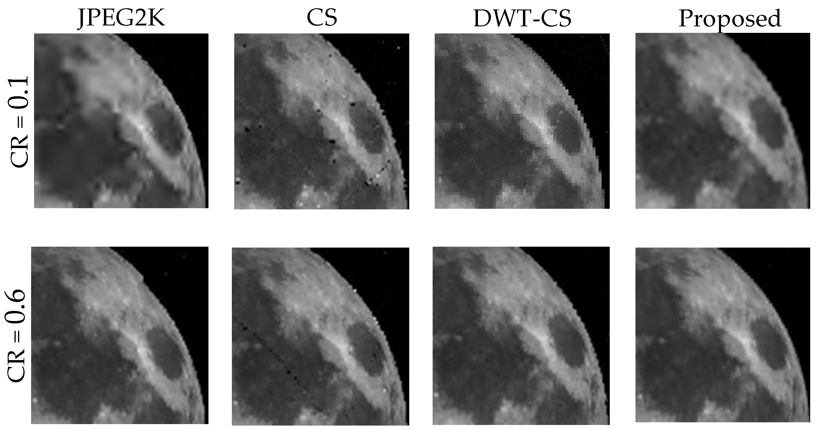
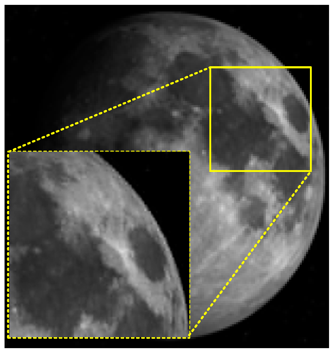
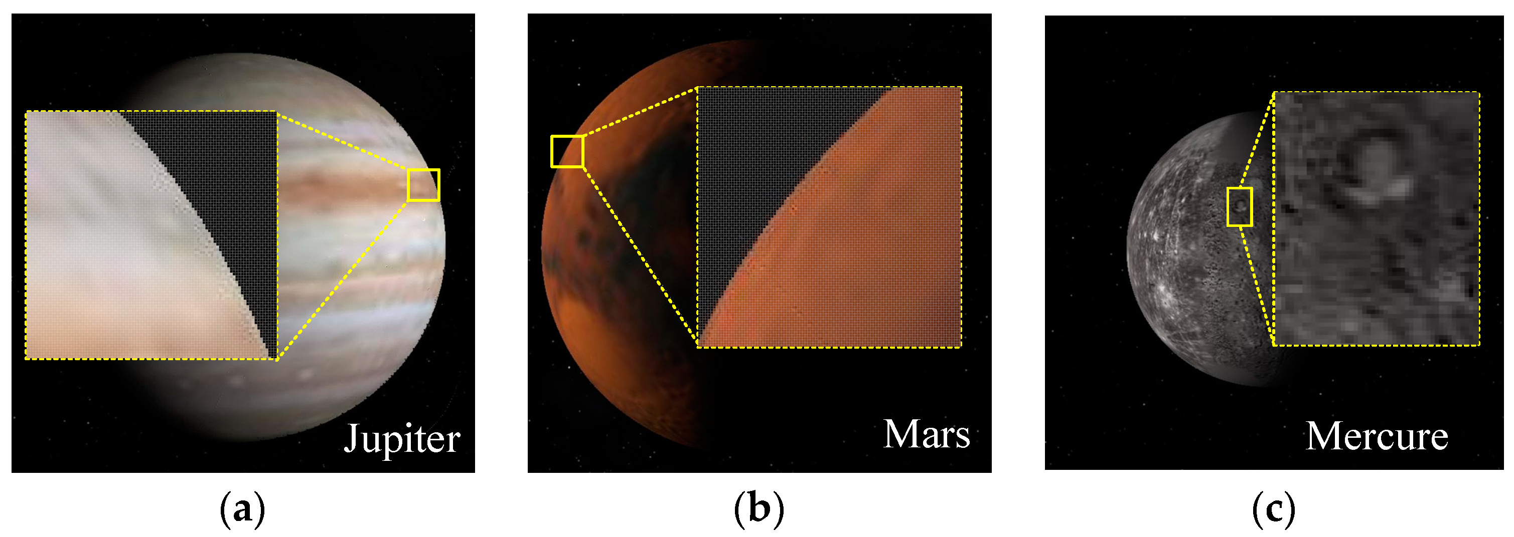
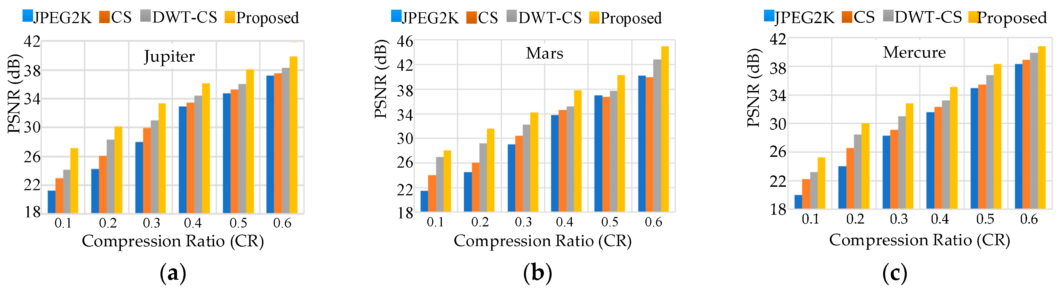
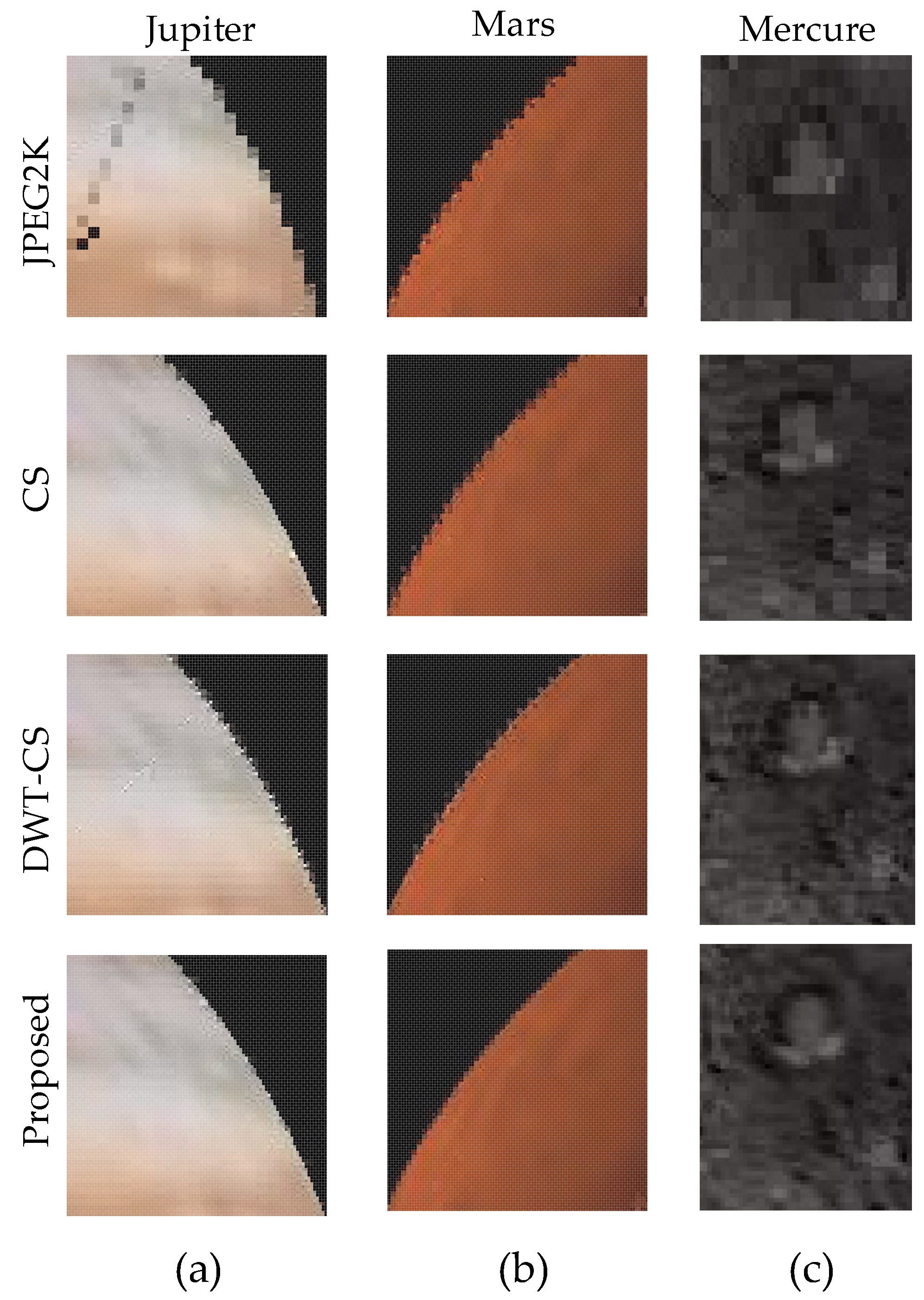
In deep space exploration, our focus in the image compression of the optical sensor system is the compression (sampling) process. CS uses sparsity to perform linear compression at encoding, and nonlinear reconstruction at decoding. It effectively saves the cost of encoding and transfers the calculation cost to decoding. Therefore, it is highly suitable for remotely sensed astronomical images with a large amount of data and high redundancy in deep space exploration.
The encoding of CS has two main parts: The sparseness and the measurement matrix. The sparseness of DWT is better than that of other sparse bases, but conventional sparse vectors do not define a structure for wavelet coefficients. A method was proposed to average the wavelet coefficient matrix to construct sparse vectors [
40]. Such methods do not consider the dependency between sub-bands and the direction information of high-frequency sub-bands, which will lead to poor performance in image compression. However, the fixed and improved measurement matrix cannot optimally allocate the measurement rate, and no measurement matrix is available to consider both sparse vectors and their elements. Therefore, we combine a new structured manner sparse vector and an optimized measurement matrix to design an optimal sampling scheme. The details of our proposed algorithm are as follows.
3.1. A New Sparse Vector Based on the Rearrangement of Wavelet Coefficients
The real signal in nature has sparseness in the transform domain. We can perform compression sampling for the sparse signal. The sparse representation is the essential premise and theoretical basis of CS. In this section, we construct a new sparse vector by rearranging the wavelet coefficients according to the energy distribution of the image after DWT.
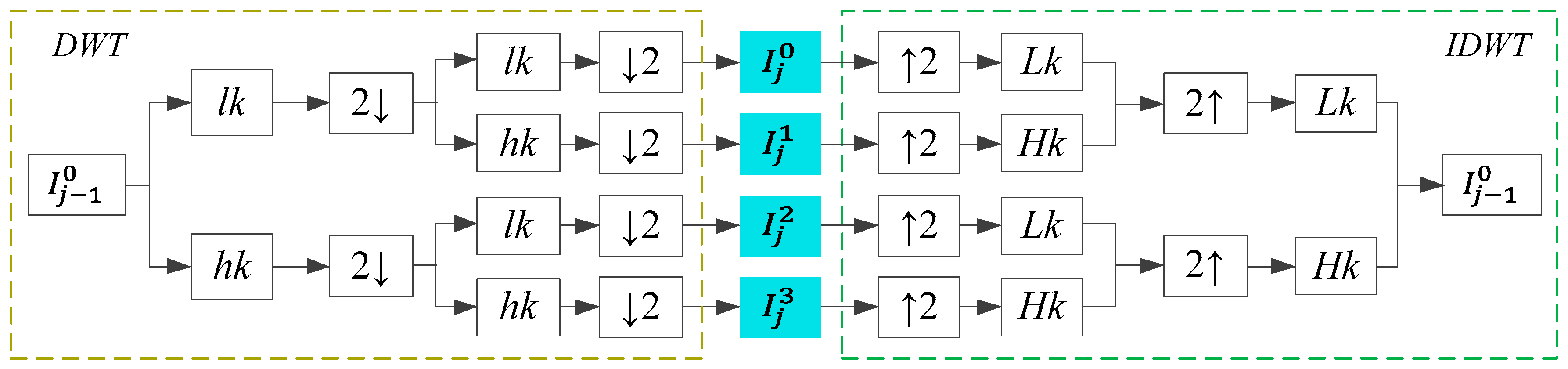
For a given remotely sensed astronomical image , the j-level DWT is applied to obtain the transformed image , which has sub-bands. The size of satisfies and , where and are natural numbers. The dimension of the i-level sub-band is . includes the low-frequency sub-band , which reflects the approximate information of the image, and high-frequency sub-bands ,, and , , reflecting the detailed information.
Figure 2a shows the tree structure of the three-level DWT. Low- and high-frequency sub-bands
and
are at the upper-left and bottom-right corners, respectively. There is a parent–child relationship between sub-bands. The direction of the arrow is from parent to child. Except for
,
,
, and
, one parent node
corresponds to four child nodes:
,
,
, and
. In low-frequency sub-band
, each node has only three child nodes:
,
, and
. When
,
, and
are regarded as parent sub-bands, the corresponding child sub-bands are
,
, and
, respectively. Similarly,
,
, and
are child sub-bands of
,
, and
, respectively. High-frequency sub-bands
,
, and
have no child sub-band. The idea of this parent–child relationship is that the parent sub-band node and the corresponding child sub-band nodes reflect the same area information of the image. The parent sub-band has a higher importance than the child sub-band. At the same level of sub-bands, the low-frequency has the highest importance, and the importance of high frequency sub-bands, in descending order, is
,
, and
[
41]. The parent–child relationship is the basis for calculation of the texture detailed complexity and design of the measurement matrix.
We design a data structure to represent sparse vector,
, according to the parent–child relationship.
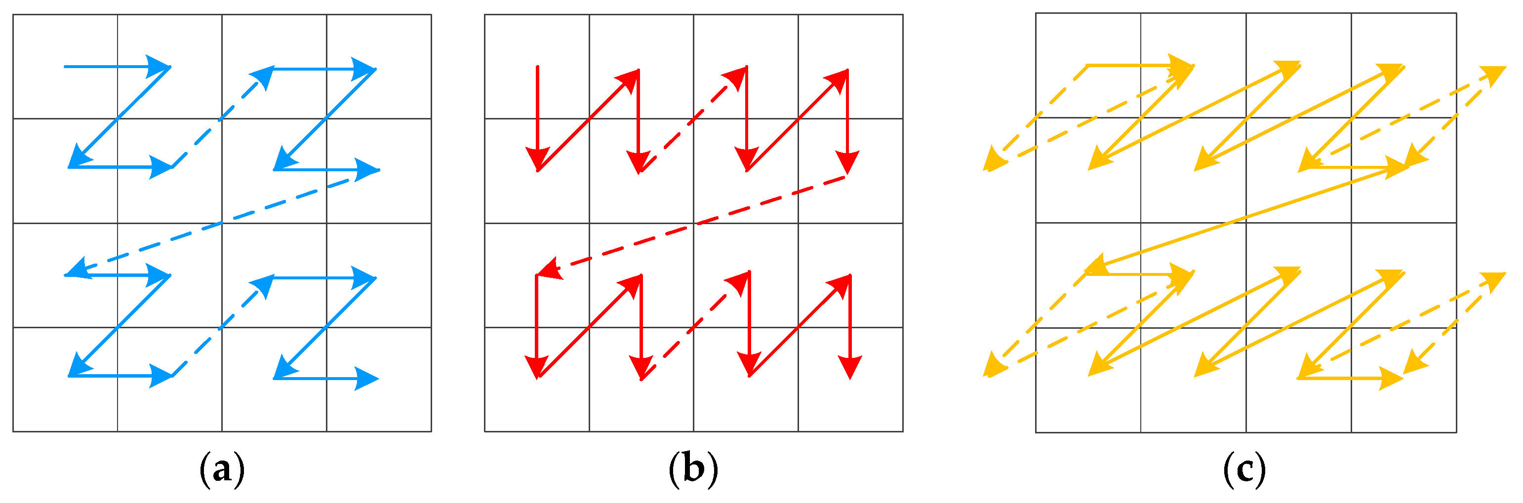
Figure 2b shows the first column,
of the sparse vector,
, and its arrangement order is as follows (j = 3):
where
,
, and
represent the horizontal, vertical, and diagonal z-scan modes, respectively. For example,
represents the diagonal z-scan mode to arrange the coefficients of the block in
. When we design a sparse vector, we must specify the block-scanning mode. This is based on the direction information of the high-frequency sub-bands. The horizontal z-scan mode is used for
, and reflects horizontal direction information; the vertical z-scan mode is used for
, and reflects vertical direction information; sub-band
, which reflects diagonal direction information, adopts the diagonal z-scan mode. Conventional CS sampling (measurement) is performed on each column (or each column of the sub-bands) of the coefficient matrix obtained by the DWT of the image [
42,
43]. High-frequency sub-bands contain the direction information of the image [
44]. The performance of CS can be further improved if this characteristic can be used. Therefore, we use different scanning modes for blocks in high-frequency sub-bands. The horizontal, vertical, and diagonal z-scan modes are shown in
Figure 3. The solid line in
Figure 3c represents the actual scan order.
In the new sparse vector, the number of elements contained in
is
where
. The new sparse vector is
Table 1 shows the number of sparse vectors and their lengths for different wavelet decomposition levels.
3.2. Measurement Matrix with Double Allocation Strategy
The measurement matrix is used to observe the high-dimensional original signal to obtain the low-dimensional compressed signal. That is, the original signal is projected onto the measurement matrix to obtain the compressed signal. In this section, depending on the parent–child relationship between sub-bands and scanning modes for high-frequency sub-bands, we design a new sparse vector to achieve an optimal measurement rate allocation scheme. The new sparse vector has some unique characteristics. Each sparse vector is composed of a low-frequency sub-band coefficient and multiple high-frequency sub-band coefficients. Elements in the same sparse vector have different importance degrees. The elements of each sparse vector are the frequency information of the same area in the image. The sparse vectors have different importance to image reconstruction; image areas with rich texture are more important.
Therefore, we propose an optimized measurement matrix with a double allocation of measurement rates, which has the advantage that the effects of sparse vectors and their elements on the measurement rate allocation are considered simultaneously. For different sparse vectors, we allocate higher measurement rates to important sparse vectors. In a sparse vector, more weight is given to important elements. The main steps are as follows.
An random Gaussian matrix is constructed.
In a sparse vector, the importance of the elements decreases from the front to the back. Increasing the coefficient of the first half of the measurement matrix can preserve more important information of the image. To do this, and to satisfy the incoherence requirement of any two columns of the measurement matrix, we introduce an
optimized matrix,
where
and
are different prime numbers. Since
and
are relatively prime, any two columns of
are incoherent [
45,
46].
The upper left part of is dot-multiplied with , and other coefficients of remain unchanged, to obtain an optimized measurement matrix . Because and , the coefficients of the upper-left part of are increased.
is the size of . It is determined by the measurement rate of each sparse vector. When the total measurement rate is certain, the measurement rate is allocated according to the texture detail complexity of the image. We calculate as follows.
The elements in the sparse vector correspond to the frequency information of the same area in the image. The high-frequency coefficients reflect the detailed information. The energy of high-frequency coefficients is defined to describe the texture detailed complexity of the sparse vector. Taking
as an example, the energy of the high-frequency coefficients of
is
where
represents the i-th element in
.
If the total measurement rate is
, then the total measurement number is
is divided into two parts: Adaptive distribution and fixed distribution. The measurement number used to adaptively allocate according to the complexity of the texture is
The measurement number of fixed allocation is
i.e.,
is evenly allocated to each sparse vector.
The higher the texture detailed complexity, the higher measurement rates are allocated to ensure retention of more details. Image areas with low texture detailed complexity, such as the background and smooth surface areas, are allocated lower measurement rates. The measurement rate is adaptively allocated according to the texture detailed complexity. A linear measurement rate allocation scheme is established based on this principle. The measurement number of the sparse vector
is
where
is the number of sparse vectors, and
is a proportionality coefficient. Then the measurement number of
is
and the final measurement number of
is
, i.e.,
The sparse vectors are compressed by the optimized measurement matrix, and the compressed value of
is


