
Changes in Meadow Phenology in Response to Grazing Management at Multiple Scales of Measurement


Abstract
:
1. Introduction
2. Methods and Materials
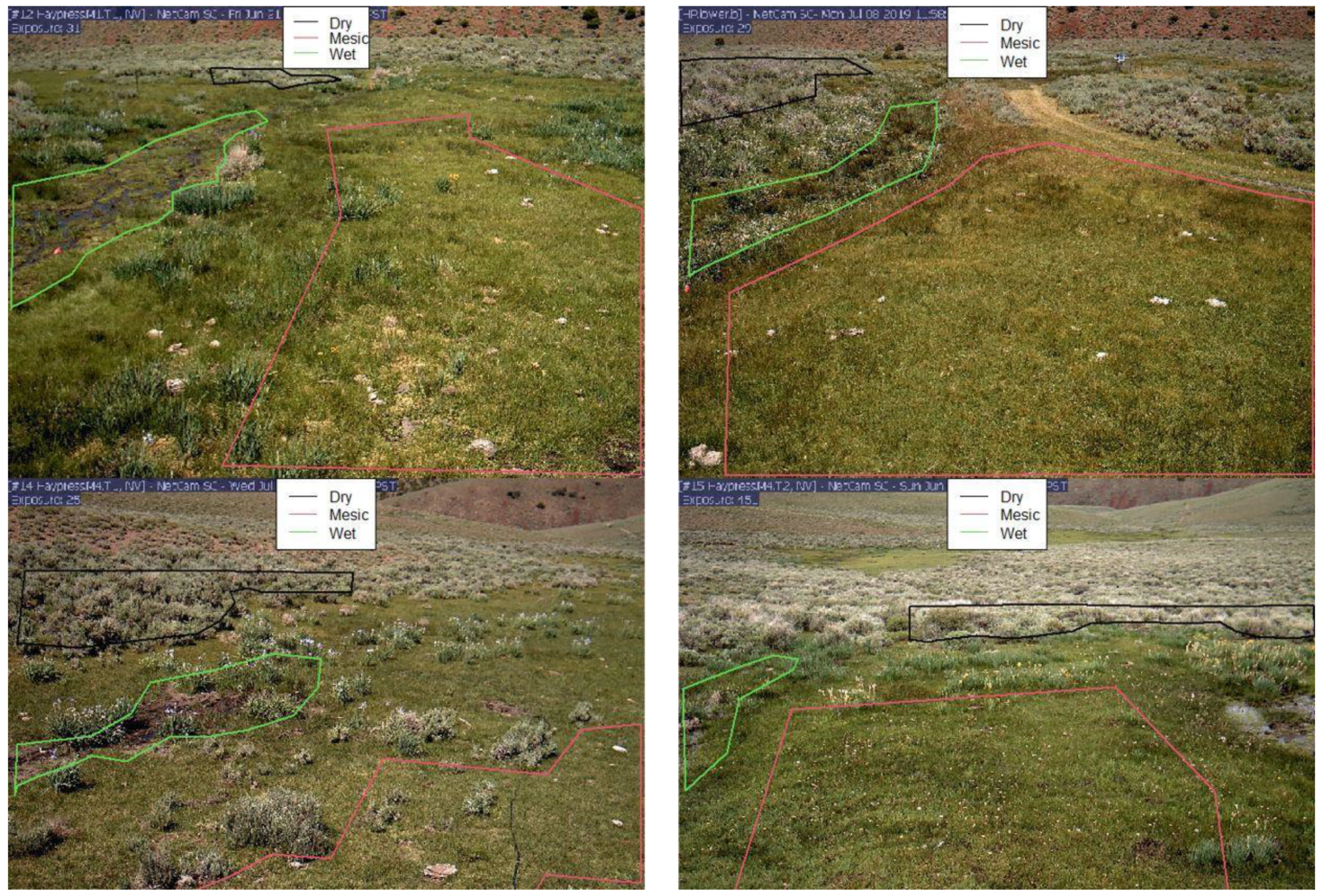
2.1. Site Description and Treatments
2.2. Field Methodology
2.3. Phenocam and Landsat Methodology
2.4. Statistical Methodology
3. Results
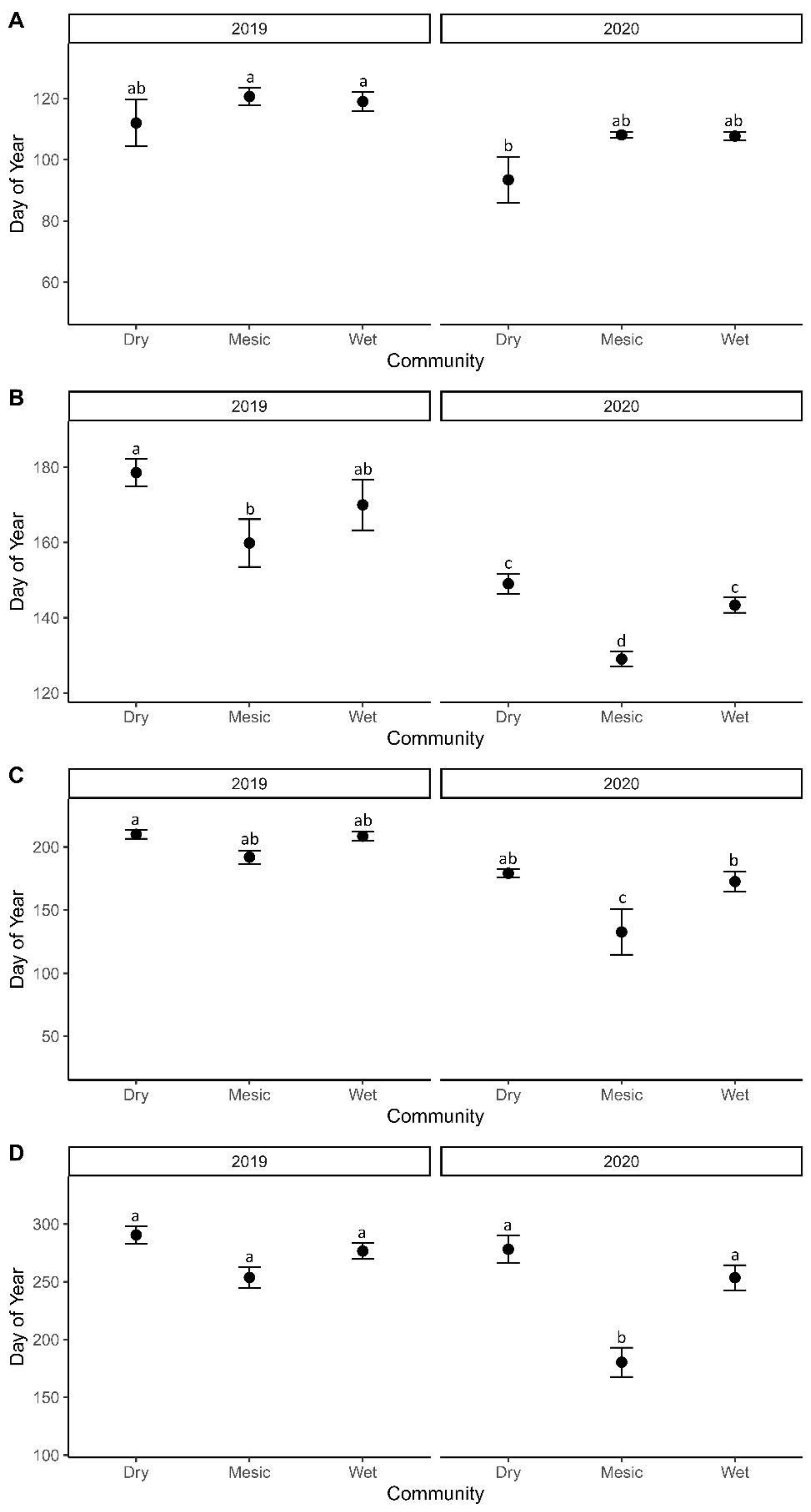
3.1. Phenology Stage Modeling
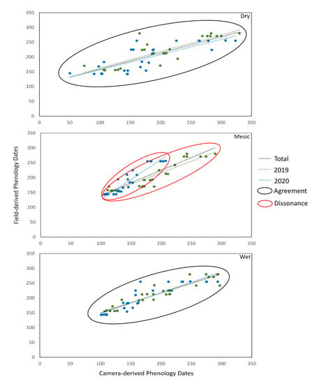
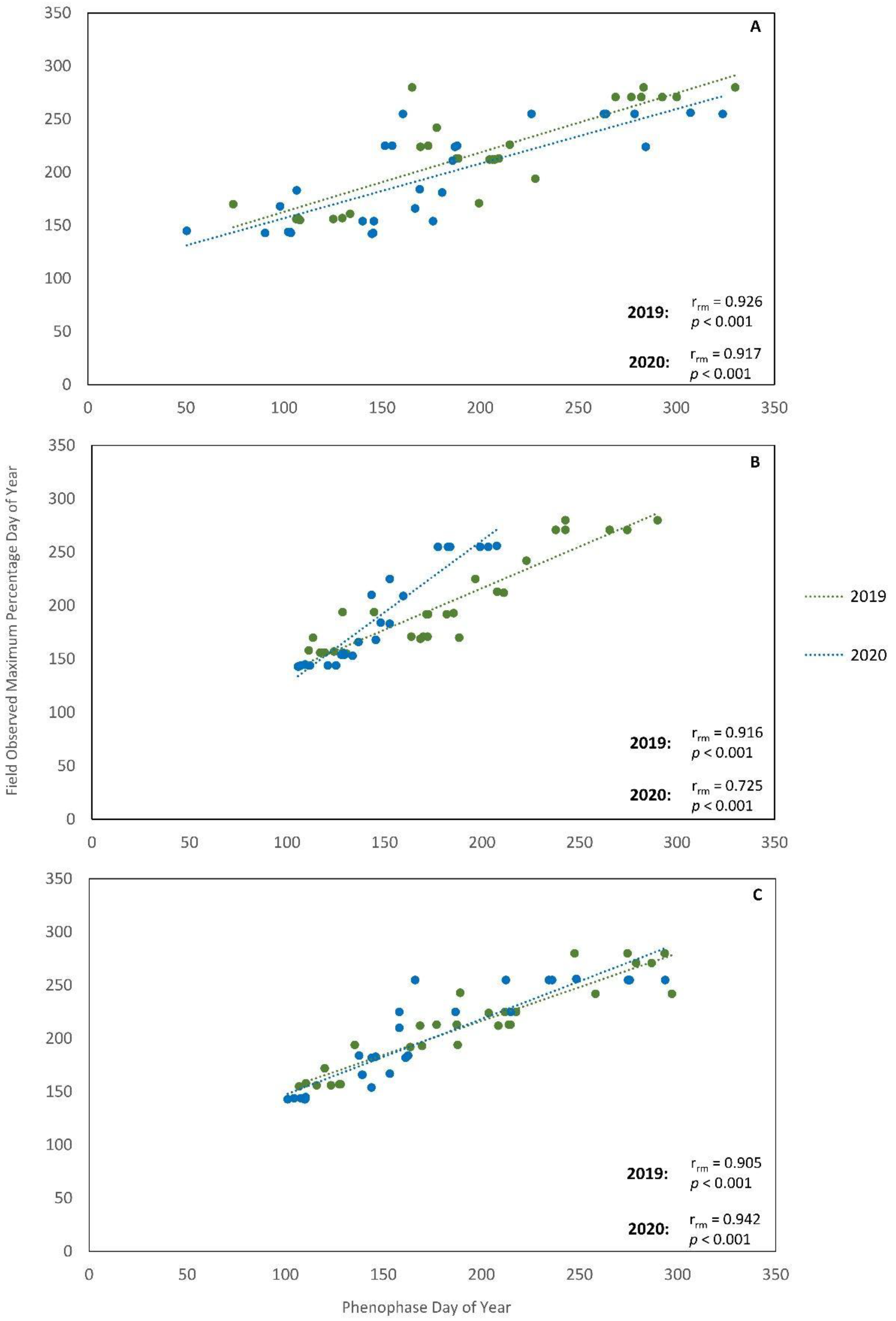
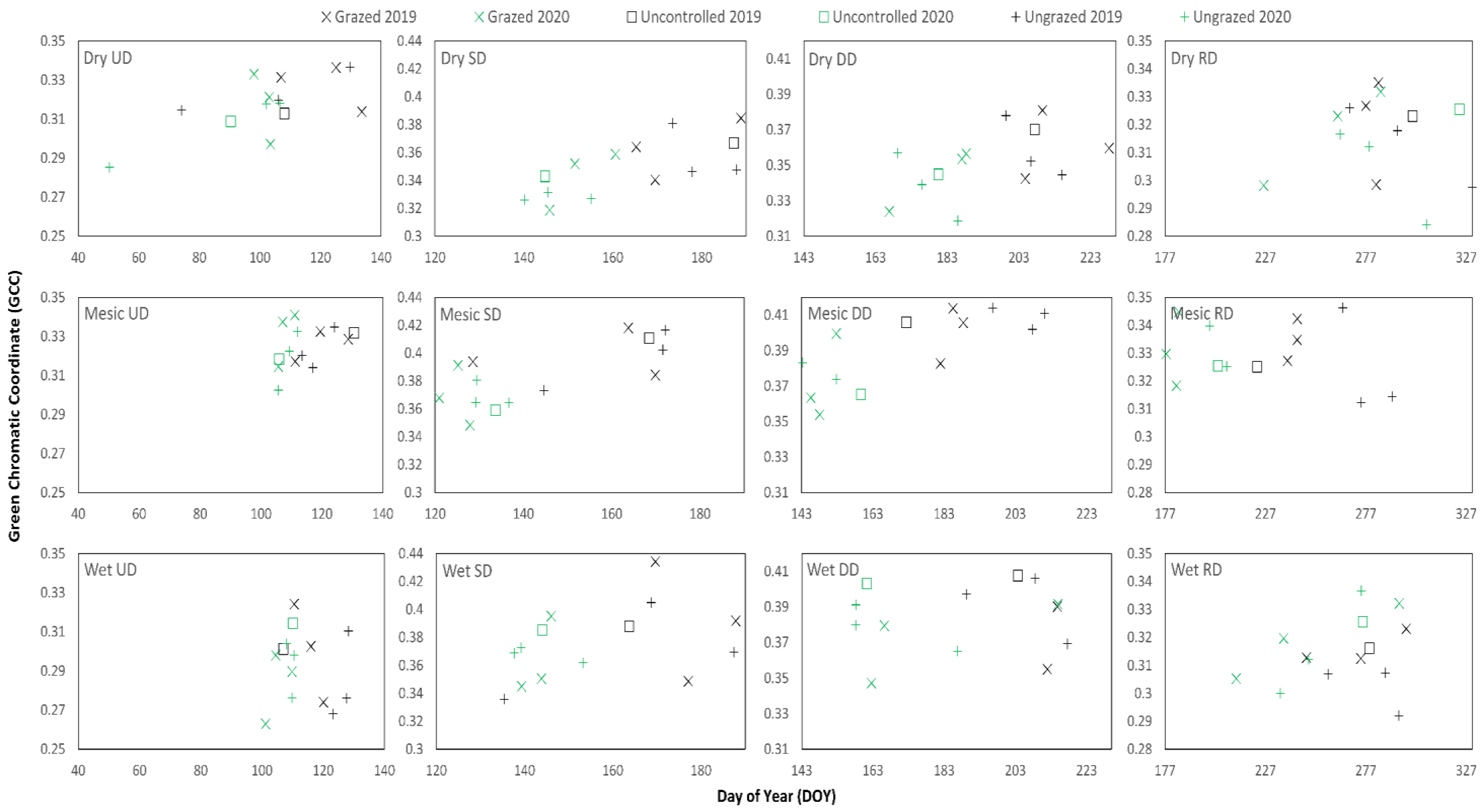
3.2. Phenocam and Field-Based Metrics and Correlations
3.3. Landsat and Phenocam Relationship
3.4. Soil Moisture
4. Discussion
4.1. Influences of Climatic and Community Variables
4.2. Grazing Impact on Phenology
4.3. Relationships between Spatial Resolutions
5. Conclusions
Supplementary Materials
Author Contributions
Funding
Data Availability Statement
Acknowledgments
Conflicts of Interest
References
- Naiman, R.J.; Decamps, H. The ecology of interfaces: Riparian zones. Annu. Rev. Ecol. Syst. 1997, 28, 621–658. [Google Scholar] [CrossRef] [Green Version]
- Fesenmyer, K.A.; Dauwalter, D.C.; Evans, C.; Allai, T. Livestock Management, beaver, and climate influences on riparian vegetation in a semi-arid landscape. PLoS ONE 2018, 13, e0208928. [Google Scholar] [CrossRef] [PubMed]
- Sabo, J.L.; Sponseller, R.; Dixon, M.; Gade, K.; Harms, T.; Heffernan, J.; Jani, A.; Katz, G.; Soykan, C.; Watts, J. Riparian zones increase regional species richness by harboring different, not more, species. Ecology 2005, 86, 56–62. [Google Scholar] [CrossRef]
- Tate, K.W.; Atwill, E.R.; Bartolome, J.W.; Nader, G. Significant Escherichia coli attenuation by vegetative buffers on annual grasslands. J. Environ. Qual. 2006, 35, 795–805. [Google Scholar] [CrossRef] [PubMed] [Green Version]
- Belsky, A.J.; Matzke, A.; Uselman, S. Survey of livestock influences on stream and riparian ecosystems in the Western United States. J. Soil Water Conserv. 1999, 54, 419–431. [Google Scholar]
- Knopf, F.L.; Johnson, R.R.; Rich, T.; Samson, F.B.; Szaro, R.C. Conservation of riparian ecosystems in the United States. Wilson Bull. 1988, 100, 272–284. [Google Scholar]
- Kondolf, G.M.; Kattelmann, R.; Embury, M.; Erman, D.C. Status of Riparian Habitat. In Sierra Nevada Ecosystem Project: Final report to Congress; University of California: Davis, CA, USA, 1996; Volume 36, pp. 1009–1030. [Google Scholar]
- Kauffman, J.B.; Krueger, W.C. Livestock impacts on riparian ecosystems and streamside management implications—A review. J. Range Manag. 1984, 37, 430–438. [Google Scholar] [CrossRef]
- Agouridis, C.T.; Workman, S.R.; Warner, R.C.; Jennings, G.D. Livestock grazing management impacts on stream water quality: A review. J. Am. Water Resour. Assoc. 2005, 41, 591–606. [Google Scholar] [CrossRef]
- Walrath, J.D.; Dauwalter, D.C.; Reinke, D. Influence of stream condition on habitat diversity and fish assemblages in an impaired upper snake river basin watershed. Trans. Am. Fish. Soc. 2016, 145, 821–834. [Google Scholar] [CrossRef]
- Eisenmann, H.; Harms, H.; Meckenstock, R.; Meyer, E.I.; Zehnder, A.J. Grazing of a Tetrahymena Sp. on adhered bacteria in percolated columns monitored by in situ hybridization with fluorescent oligonucleotide probes. Appl. Environ. Microbiol. 1998, 64, 1264–1269. [Google Scholar] [CrossRef] [Green Version]
- Stern, M.; Quesada, M.; Stoner, K.E. Changes in composition and structure of a tropical dry forest following intermittent cattle grazing. Revista de Biología Tropical 2002, 50, 1021–1034. [Google Scholar]
- Zangerl, A.; Hamilton, J.; Miller, T.; Crofts, A.; Oxborough, K.; Berenbaum, M.; De Lucia, E. Impact of folivory on photosynthesis is greater than the sum of its holes. Proc. Natl. Acad. Sci. USA 2002, 99, 1088–1091. [Google Scholar] [CrossRef] [Green Version]
- Skaer, M.J.; Graydon, D.J.; Cushman, J.H.; Pugnaire, F. Community-level consequences of cattle grazing for an invaded grassland: Variable responses of native and exotic vegetation. J. Veg. Sci. 2013, 24, 332–343. [Google Scholar] [CrossRef]
- Browning, D.M.; Snyder, K.A.; Herrick, J.E. Plant phenology: Taking the pulse of rangelands. Rangelands 2019, 41, 129–134. [Google Scholar] [CrossRef]
- Denny, E.G.; Gerst, K.L.; Miller-Rushing, A.J.; Tierney, G.L.; Crimmins, T.M.; Enquist, C.A.; Guertin, P.; Rosemartin, A.H.; Schwartz, M.D.; Thomas, K.A. Standardized phenology monitoring methods to track plant and animal activity for science and resource management applications. Int. J. Biometeorol. 2014, 58, 591–601. [Google Scholar] [CrossRef] [PubMed] [Green Version]
- Parmesan, C. Ecological and evolutionary responses to recent climate change. Annu. Rev. Ecol. Evol. Syst. 2006, 37, 637–669. [Google Scholar] [CrossRef] [Green Version]
- Cleland, E.E.; Chuine, I.; Menzel, A.; Mooney, H.A.; Schwartz, M.D. Shifting plant phenology in response to global change. Trends Ecol. Evol. 2007, 22, 357–365. [Google Scholar] [CrossRef] [PubMed]
- Thackeray, S.J.; Sparks, T.H.; Frederiksen, M.; Burthe, S.; Bacon, P.J.; Bell, J.R.; Botham, M.S.; Brereton, T.M.; Bright, P.W.; Carvalho, L.; et al. Trophic level asynchrony in rates of phenological change for marine, freshwater and terrestrial environments. Glob. Chang. Biol. 2010, 16, 3304–3313. [Google Scholar] [CrossRef] [Green Version]
- Jensen, K.; Gutekunst, K. Effects of litter on establishment of grassland plant species: The role of seed size and successional status. Basic Appl. Ecol. 2003, 4, 579–587. [Google Scholar] [CrossRef]
- Miller-Rushing, A.J.; Hoye, T.T.; Inouye, D.W.; Post, E. The effects of phenological mismatches on demography. Philos. Trans. R. Soc. B Biol. Sci. 2010, 365, 3177–3186. [Google Scholar] [CrossRef] [PubMed] [Green Version]
- Fenetahun, Y.; Yuan, Y.; Xinwen, X.; Yongdong, W. Effects of grazing enclosures on species diversity, phenology, biomass, and carrying capacity in Borana Rangeland, Southern Ethiopia. Front. Ecol. Evol. 2021, 8, 623627. [Google Scholar] [CrossRef]
- Reeder, J.D.; Schuman, G.E.; Morgan, J.A.; Lecain, D.R. Response of organic and inorganic carbon and nitrogen to long-term grazing of the shortgrass steppe. Environ. Manag. 2004, 33, 485–495. [Google Scholar] [CrossRef]
- Li, Y.; Zhao, X.; Chen, Y.; Luo, Y.; Wang, S. Effects of grazing exclusion on carbon sequestration and the associated vegetation and soil characteristics at a semi-arid desertified sandy site in Inner Mongolia, Northern China. Can. J. Soil Sci. 2012, 92, 807–819. [Google Scholar] [CrossRef]
- Zhu, J.; Zhang, Y.; Liu, Y. Effects of short-term grazing exclusion on plant phenology and reproductive succession in a Tibetan Alpine Meadow. Sci. Rep. 2016, 6, 27781. [Google Scholar] [CrossRef] [PubMed] [Green Version]
- Glynn, P.D.; Owen, T.W. Review of the USA National Phenology Network. U.S. Geol. Surv. Circ. 2015, 1411, 2–4. [Google Scholar] [CrossRef] [Green Version]
- Browning, D.M.; Karl, J.W.; Morin, D.; Richardson, A.D.; Tweedie, C.E. Phenocams bridge the gap between field and satellite observations in an arid grassland ecosystem. Remote Sens. 2017, 9, 1071. [Google Scholar] [CrossRef] [Green Version]
- Browning, D.M.; Rango, A.; Karl, J.W.; Laney, C.M.; Vivoni, E.R.; Tweedie, C.E. Emerging technological and cultural shifts advancing drylands research and management. Front. Ecol. Environ. 2015, 13, 52–60. [Google Scholar] [CrossRef] [Green Version]
- Brown, T.B.; Hultine, K.R.; Steltzer, H.; Denny, E.G.; Denslow, M.W.; Granados, J.; Henderson, S.; Moore, D.; Nagai, S.; SanClements, M.; et al. Using phenocams to monitor our changing earth: Toward a global phenocam network. Front. Ecol. Environ. 2016, 14, 84–93. [Google Scholar] [CrossRef] [Green Version]
- Morisette, J.T.; Richardson, A.D.; Knapp, A.K.; Fisher, J.I.; Graham, E.A.; Abatzoglou, J.; Wilson, B.E.; Breshears, D.D.; Henebry, G.M.; Hanes, J.M. Tracking the rhythm of the seasons in the face of global change: Phenological research in the 21st century. Front. Ecol. Environ. 2009, 7, 253–260. [Google Scholar] [CrossRef] [Green Version]
- Melaas, E.K.; Sulla-Menashe, D.; Gray, J.M.; Black, T.A.; Morin, T.H.; Richardson, A.D.; Friedl, M.A. Multisite analysis of land surface phenology in North American temperate and boreal deciduous forests from landsat. Remote Sens. Environ. 2016, 186, 452–464. [Google Scholar] [CrossRef]
- Klosterman, S.; Hufkens, K.; Gray, J.; Melaas, E.; Sonnentag, O.; Lavine, I.; Mitchell, L.; Norman, R.; Friedl, M.; Richardson, A. Evaluating remote sensing of deciduous forest phenology at multiple spatial scales using phenocam imagery. Biogeosciences 2014, 11, 4305–4320. [Google Scholar] [CrossRef] [Green Version]
- Forkel, M.; Migliavacca, M.; Thonicke, K.; Reichstein, M.; Schaphoff, S.; Weber, U.; Carvalhais, N. Codominant water control on global interannual variability and trends in land surface phenology and greenness. Glob. Chang. Biol. 2015, 21, 3414–3435. [Google Scholar] [CrossRef] [PubMed]
- Filippa, G.; Cremonese, E.; Migliavacca, M.; Galvagno, M.; Sonnentag, O.; Humphreys, E.; Hufkens, K.; Ryu, Y.; Verfaillie, J.; di Cella, U.M. NDVI derived from near-infrared-enabled digital cameras: Applicability across different plant functional types. Agric. For. Meteorol. 2018, 249, 275–285. [Google Scholar] [CrossRef]
- Weltzin, J.F.; Tissue, D.T. Resource pulses in arid environments: Patterns of rain, patterns of life. N. Phytol. 2003, 157, 171–173. [Google Scholar] [CrossRef] [PubMed]
- Schwinning, S.; Sala, O.E.; Loik, M.E.; Ehleringer, J.R. Thresholds, memory, and seasonality: Understanding pulse dynamics in arid/semi-arid ecosystems. Oecologia 2004, 141, 191–193. [Google Scholar] [CrossRef] [PubMed]
- Waitz, Y.; Wasserstrom, H.; Hanin, N.; Landau, N.; Faraj, T.; Barzilai, M.; Ziffer-Berger, J.; Barazani, O. Close association between flowering time and aridity gradient for sarcopoterium spinosum in Israel. J. Arid Environ. 2021, 188, 104468. [Google Scholar] [CrossRef]
- Sonnentag, O.; Hufkens, K.; Teshera-Sterne, C.; Young, A.M.; Friedl, M.; Braswell, B.H.; Milliman, T.; O’Keefe, J.; Richardson, A.D. Digital repeat photography for phenological research in forest ecosystems. Agric. For. Meteorol. 2012, 152, 159–177. [Google Scholar] [CrossRef]
- Richardson, A.D.; Hufkens, K.; Milliman, T.; Frolking, S. Intercomparison of phenological transition dates derived from the phenocam dataset V1. 0 and modis satellite remote sensing. Sci. Rep. 2018, 8, 1–12. [Google Scholar] [CrossRef] [Green Version]
- Melaas, E.K.; Sulla-Menashe, D.J.; Gray, J.; Friedl, M.A. Using three decades of landsat data to characterize changes and vulnerability of temperate and boreal forest phenology to climate change. In Proceedings of the AGU Fall Meeting Abstracts, San Francisco, CA, USA, 14–18 December 2015; p. B21G–0548. [Google Scholar]
- Hufkens, K.; Richardson, A.; Migliavacca, M.; Frolking, S.; Braswell, B.; Milliman, T.; Friedl, M. Comparing near-Earth and satellite remote sensing based phenophase estimates: An analysis using multiple webcams and modis. In Proceedings of the AGU Fall Meeting Abstracts, San Francisco, CA, USA, 13–17 December 2010; p. B52C-03. [Google Scholar]
- Patten, D.T.; Rouse, L.; Stromberg, J.C. Isolated spring wetlands in the great Basin and Mojave Deserts, USA: Potential response of vegetation to groundwater withdrawal. Environ. Manag. 2008, 41, 398–413. [Google Scholar] [CrossRef]
- Snyder, K.A.; Huntington, J.L.; Wehan, B.L.; Morton, C.G.; Stringham, T.K. Comparison of landsat and land-based phenology camera normalized difference vegetation index (NDVI) for dominant plant communities in the Great Basin. Sensors 2019, 19, 1139. [Google Scholar] [CrossRef] [Green Version]
- Huntington, J.; McGwire, K.; Morton, C.; Snyder, K.; Peterson, S.; Erickson, T.; Niswonger, R.; Carroll, R.; Smith, G.; Allen, R. Assessing the role of climate and resource management on groundwater dependent ecosystem changes in arid environments with the landsat archive. Remote Sens. Environ. 2016, 185, 186–197. [Google Scholar] [CrossRef] [Green Version]
- Soil Survey Staff Natural Resources Conservation Service USDA. Web Soil Survey. Available online: http://websoilsurvey.sc.egov.usda.gov/ (accessed on 8 May 2021).
- Herrick, J.E.; Van Zee, J.W.; Havstad, K.M.; Burkett, L.M.; Whitford, W.G. Monitoring Manual for Grassland, Shrubland and Savanna Ecosystems. Volume II: Design, Supplementary Methods and Interpretation; USDA-ARS Jornada Experimental Range: Las Cruces, NM, USA, 2005; ISBN 0975555200.
- Hall, F.D.; Bryant, L. Herbaceous Stubble Height as a Warning of Impending Cattle Grazing Damage to Riparian Areas; United States Department of Agriculture, Forest Service, Pacific Northwest Research Station: Portland, OR, USA, 1995.
- Moore, K.; Moser, L.E.; Vogel, K.P.; Waller, S.S.; Johnson, B.; Pedersen, J.F. Describing and quantifying growth stages of perennial forage grasses. Agron. J. 1991, 83, 1073–1077. [Google Scholar] [CrossRef] [Green Version]
- Filippa, G.; Cremonese, E.; Migliavacca, M.; Galvagno, M.; Forkel, M.; Wingate, L.; Tomelleri, E.; Di Cella, U.M.; Richardson, A.D. Phenopix: Ar package for image-based vegetation phenology. Agric. For. Meteorol. 2016, 220, 141–150. [Google Scholar] [CrossRef] [Green Version]
- Gu, L.; Post, W.M.; Baldocchi, D.D.; Black, T.A.; Suyker, A.E.; Verma, S.B.; Vesala, T.; Wofsy, S.C. Characterizing the seasonal dynamics of plant community photosynthesis across a range of vegetation types. In Phenology of Ecosystem Processes; Springer: New York, NY, USA, 2009; pp. 35–58. [Google Scholar]
- Fox, E.W.; Ver Hoef, J.M.; Olsen, A.R. Comparing spatial regression to random forests for large environmental data sets. PLoS ONE 2020, 15, e0229509. [Google Scholar] [CrossRef] [PubMed] [Green Version]
- Cutler, D.R.; Edwards, T.C., Jr.; Beard, K.H.; Cutler, A.; Hess, K.T.; Gibson, J.; Lawler, J.J. Random forests for classification in ecology. Ecology 2007, 88, 2783–2792. [Google Scholar] [CrossRef]
- Liaw, A.; Wiener, M. Classification and regression by randomforest. R News 2002, 2, 18–22. [Google Scholar]
- R Core Team. R: A Language and Environment for Statistical Computing; R Foundation for Statistical Computing: Vienna, Austria, 2013. [Google Scholar]
- Berlow, E.L.; D’Antonio, C.M.; Reynolds, S.A. Shrub expansion in montane meadows: The interaction of local-scale disturbance and site aridity. Ecol. Appl. 2002, 12, 1103–1118. [Google Scholar] [CrossRef]
- Darrouzet-Nardi, A.; D’Antonio, C.M.; Dawson, T.E. Depth of water acquisition by invading shrubs and resident herbs in a sierra nevada meadow. Plant Soil 2006, 285, 31–43. [Google Scholar] [CrossRef]
- Denny, M.W.; Dowd, W.W.; Bilir, L.; Mach, K.J. Spreading the risk: Small-scale body temperature variation among intertidal organisms and its implications for species persistence. J. Exp. Mar. Biol. Ecol. 2011, 400, 175–190. [Google Scholar] [CrossRef]
- Osem, Y.; Perevolotsky, A.; Kigel, J. Grazing effect on diversity of annual plant communities in a semi-arid rangeland: Interactions with small-scale spatial and temporal variation in primary productivity. J. Ecol. 2002, 90, 936–946. [Google Scholar] [CrossRef]
- Zhang, T.; Xu, M.; Zhang, Y.; Zhao, T.; An, T.; Li, Y.; Sun, Y.; Chen, N.; Zhao, T.; Zhu, J.; et al. Grazing-induced increases in soil moisture maintain higher productivity during droughts in alpine meadows on the Tibetan Plateau. Agric. For. Meteorol. 2019, 269–270, 249–256. [Google Scholar] [CrossRef]
- da Silva, A.P.; Imhoff, S.; Corsi, M. Evaluation of soil compaction in an irrigated short-duration grazing system. Soil Tillage Res. 2003, 70, 83–90. [Google Scholar] [CrossRef]
- Zhao, Y.; Peth, S.; Horn, R.; Krümmelbein, J.; Ketzer, B.; Gao, Y.; Doerner, J.; Bernhofer, C.; Peng, X. Modeling grazing effects on coupled water and heat fluxes in inner Mongolia grassland. Soil Tillage Res. 2010, 109, 75–86. [Google Scholar] [CrossRef]
- Zhao, Y.; Peth, S.; Reszkowska, A.; Gan, L.; Krümmelbein, J.; Peng, X.; Horn, R. Response of soil moisture and temperature to grazing intensity in a leymus chinensis steppe, inner Mongolia. Plant Soil 2011, 340, 89–102. [Google Scholar] [CrossRef]
- Virgona, J.; Gummer, F.; Angus, J. Effects of grazing on wheat growth, yield, development, water use, and nitrogen use. Aust. J. Agric. Res. 2006, 57, 1307–1319. [Google Scholar] [CrossRef]
- Henkin, Z.; Ungar, E.; Dvash, L.; Perevolotsky, A.; Yehuda, Y.; Sternberg, M.; Voet, H.; Landau, S. Effects of cattle grazing on herbage quality in a herbaceous mediterranean rangeland. Grass Forage Sci. 2011, 66, 516–525. [Google Scholar] [CrossRef]
- Kelman, W.; Dove, H. Growth and phenology of winter wheat and oats in a dual-purpose management system. Crop Pasture Sci. 2009, 60, 921–932. [Google Scholar] [CrossRef]
- Kirkegaard, J.; Lilley, J.; Hunt, J.; Sprague, S.; Ytting, N.; Rasmussen, I.; Graham, J. Effect of defoliation by grazing or shoot removal on the root growth of field-grown wheat (Triticum Aestivum L.). Crop Pasture Sci. 2015, 66, 249–259. [Google Scholar] [CrossRef]


| Site | Camera Viewshed (ha) | Meadow Area (ha) | Lat/Long (Decimal Degrees) | Camera Orientation (Cardinal Direction) |
|---|---|---|---|---|
| Upper A | 0.09 | 0.64 | 39.317479/−117.697128 | NE |
| Upper B | 0.11 | 0.29 | 39.315936/−117.698013 | NNW |
| Middle A | 0.10 | 0.73 | 39.322538/−117.703238 | NE |
| Middle B | 0.04 | 0.11 | 39.320682/−117.703979 | NNE |
| Lower A | 0.18 | 0.56 | 39.331126/−117.701456 | NNE |
| Lower B | 0.15 | 0.66 | 39.330403/−117.701739 | NNW |
| Uncontrolled | 0.12 | 0.33 | 39.325874/−117.688641 | E |
| Variable | Definition |
|---|---|
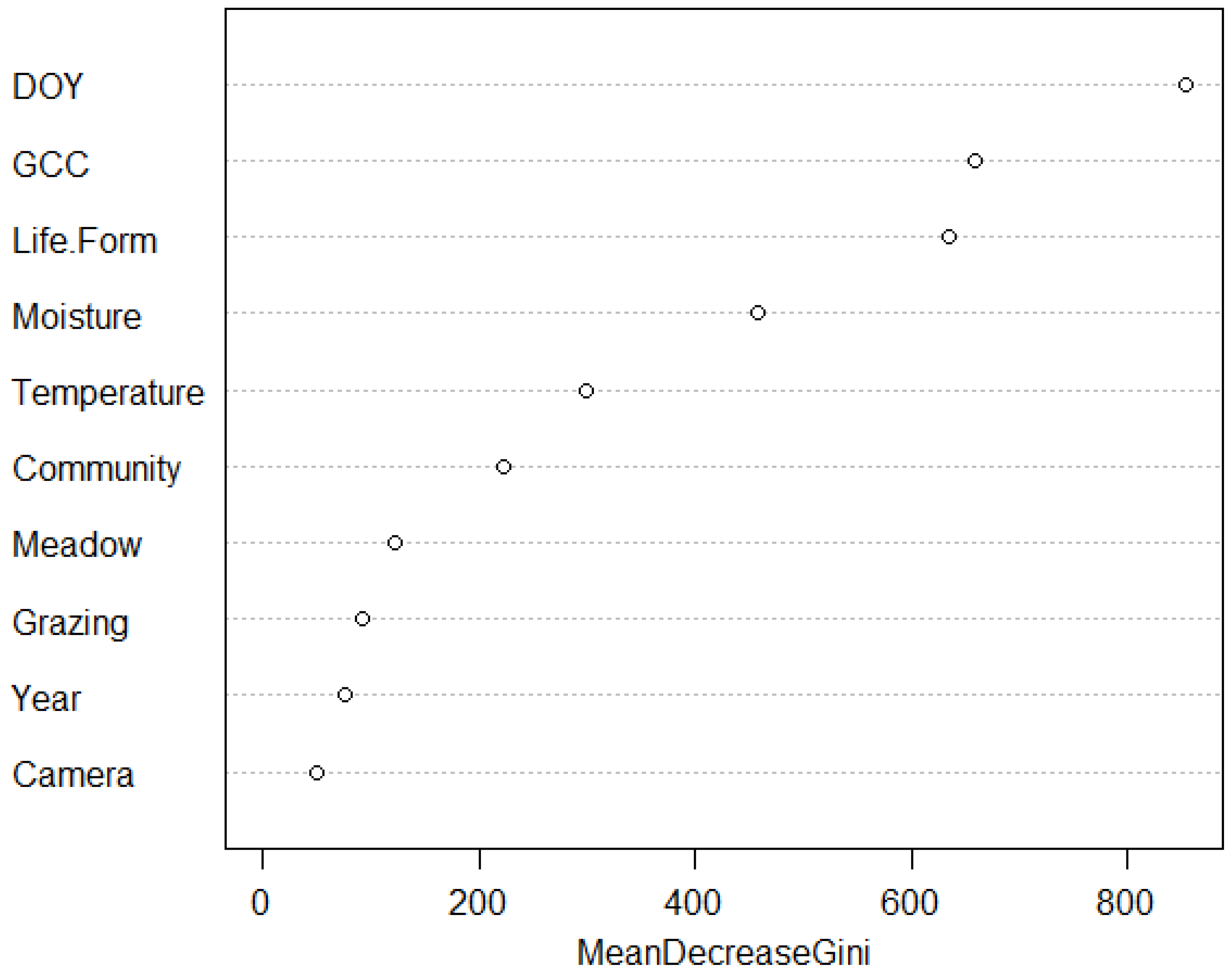
| DOY | Day of year |
| GCC | Green Chromatic Coordinate value derived from phenocams |
| Life.Form | Life-form (i.e., graminoid, forb, graminoid-like, shrub) |
| Moisture | Soil moisture |
| Temperature | Temperature (degrees Celsius) |
| Community | Plant community type (i.e., dry, mesic, wet) |
| Grazing | Grazing intensity (i.e., uncontrolled grazing, managed grazing, ungrazed) |
| Year | Year of data collection |
| Meadow | Meadow of data collection (Upper, Middle, etc.) |
| Camera | Portion of meadow (i.e., high elevation, low elevation) |
| Variable | Analysis | UD | SD | DD | RD |
|---|---|---|---|---|---|
| Year | ANOVA Prob > F | 0.0006 | <0.0001 | <0.0001 | 0.0001 |
| Community | ANOVA Prob > F | 0.06 | 0.0005 | 0.0012 | <0.0001 |
| Grazing/Year Interaction | ANOVA Prob > F | 0.992 | 0.929 | 0.289 | 0.164 |
| Meadow | ANOVA Prob > F | 0.06 | 0.332 | 0.359 | 0.067 |
| Variable | Analysis | L | I | S | D |
|---|---|---|---|---|---|
| Year | ANOVA Prob > F | <0.0001 | <0.0001 | 0.0016 | 0.003 |
| Community | ANOVA Prob > F | 0.522 | 0.0525 | 0.0248 | 0.244 |
| Grazing/Year Interaction | ANOVA Prob > F | 0.782 | 0.588 | 0.945 | 0.889 |
| Meadow | ANOVA Prob > F | 0.067 | 0.377 | 0.947 | 0.092 |
| Year | Meadow | Pearson’s r | RMSE | Prob > F |
|---|---|---|---|---|
| 2019 | Lower A | 0.963365 | 0.107 | >0.0001 |
| Lower B | 0.983981 | 0.104 | >0.0001 | |
| Middle A | 0.978051 | 0.087 | >0.0001 | |
| Middle B | 0.958376 | 0.075 | >0.0001 | |
| Upper A | 0.911001 | 0.061 | >0.0001 | |
| Upper B | 0.991294 | 0.137 | >0.0001 | |
| Uncontrolled | 0.970543 | 0.075 | >0.0001 | |
| 2020 | Lower A | 0.946754 | 0.065 | >0.0001 |
| Lower B | 0.982728 | 0.061 | >0.0001 | |
| Middle A | 0.950454 | 0.056 | >0.0001 | |
| Middle B | 0.913333 | 0.039 | >0.0001 | |
| Upper A | 0.912522 | 0.08 | >0.0001 | |
| Upper B | 0.966456 | 0.087 | >0.0001 | |
| Uncontrolled | 0.945573 | 0.059 | >0.0001 |
Publisher’s Note: MDPI stays neutral with regard to jurisdictional claims in published maps and institutional affiliations. |
© 2021 by the authors. Licensee MDPI, Basel, Switzerland. This article is an open access article distributed under the terms and conditions of the Creative Commons Attribution (CC BY) license (https://creativecommons.org/licenses/by/4.0/).
Share and Cite
Richardson, W.; Stringham, T.K.; Lieurance, W.; Snyder, K.A. Changes in Meadow Phenology in Response to Grazing Management at Multiple Scales of Measurement. Remote Sens. 2021, 13, 4028. https://doi.org/10.3390/rs13204028
Richardson W, Stringham TK, Lieurance W, Snyder KA. Changes in Meadow Phenology in Response to Grazing Management at Multiple Scales of Measurement. Remote Sensing. 2021; 13(20):4028. https://doi.org/10.3390/rs13204028
Chicago/Turabian StyleRichardson, William, Tamzen K. Stringham, Wade Lieurance, and Keirith A. Snyder. 2021. "Changes in Meadow Phenology in Response to Grazing Management at Multiple Scales of Measurement" Remote Sensing 13, no. 20: 4028. https://doi.org/10.3390/rs13204028
APA StyleRichardson, W., Stringham, T. K., Lieurance, W., & Snyder, K. A. (2021). Changes in Meadow Phenology in Response to Grazing Management at Multiple Scales of Measurement. Remote Sensing, 13(20), 4028. https://doi.org/10.3390/rs13204028