1. Introduction
Change detection in the field of remote sensing is the process of identifying differences in the state of an object or phenomenon by observing it at different subsequent times [
1]. The nature of this task thus requires the usage of methods and algorithms that compare two or more satellite images of the same scene and produce results that can either map changes pixel by pixel or provide an overall classification of the input data as including or not relevant changes within the analyzed area.
Specifically, change detection applied to urban areas [
2,
3] is an interesting case study as it aims at monitoring differences in land cover due to urban expansion and spread over the years in a more automated way. Although a large variety of methods exists and has been classified and discussed [
4,
5,
6], and classical methods based on pixel-difference vectors are constantly developed and studied [
7], the deep learning approach to this problem is currently object of active research and ranges from the design of innovative methods exploiting conditional generative adversarial networks (cGANs) [
8] to more complex methods that obtain fine change detection results starting from coarse scene classification [
9]. With the advent of GPUs and heterogeneous computing, the computational load of deep learning models for Earth Observation is not prohibitive as in the past, due to the considerable reduction of training time. This scenario allows inspecting the performance of several algorithms in a more efficient way, without dealing with tight restrictions. In particular, convolutional neural networks (CNNs) can easily exploit the different architecture of these devices with respect to traditional CPUs and allow achieving valuable results in shorter time.
At the same time, the training of models with a high level of generalization capabilities is extremely challenging, due to the changing urban patterns from a country to another. In addition, vegetation and seasonal changes often represent a source of contamination that cannot be easily removed, and contribute to lower the performance of efficient convolutional neural networks.
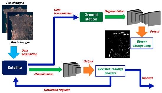
In this scenario, performing change detection with CNNs has the objective of providing a fast and useful analysis of an area that can be integrated into traditional post-processing workflows on the ground stations, which combine results from several algorithms to obtain a final map of all the changes present in the scene. This objective can be achieved with two different approaches: semantic segmentation and classification. The first approach is generally suitable for the full analysis on ground: the acquired data are downloaded at the ground facilities and the deep learning algorithm provides a detailed map of all the changes detected within the area. The second approach is onboard-oriented, as it aims to evaluate the change content of a scene and transmit such estimation to the ground stations; the latter can further decide whether to download or not the new acquired data for further analyses. Specific monitoring tasks can be planned by exploiting the onboard processing to filter the interesting data only, thus mitigating the download bottleneck.
The aim of this study is to provide high performance algorithms that can be exploited by both private companies (which usually have more complex change detection workflows) and academic institutions (for research studies). With this purpose in mind, only free-access tools have been used, as well as public data collected by the Sentinel-2 satellites.
2. The Sentinel-2 Mission
The Sentinel-2 mission consists of a constellation of two twin satellites flying in the same Sun-synchronous polar orbit but phased at at a mean altitude of 786 km, designed to give a high revisit frequency of five days at the Equator. It aims at monitoring the variability of the land surface conditions through the acquisition of high resolution multispectral images that can be exploited for land cover/change classification, atmospheric correction and cloud/snow separation.
Each satellite carries a multispectral instrument (MSI) for data acquisition [
10]. The MSI measures the Earth’s reflected radiance in 13 spectral bands: the visible and near-infrared (VNIR), and the short-wave infrared (SWIR), with three different spatial resolutions (10 m, 20 m, and 60 m). Additional information is provided in
Table 1.
Sentinel-2 data are downloaded at the ground segment, which uses several processing algorithms to obtain two types of final products, in the form of compilations of elementary granules or tiles (minimum indivisible partitions) of fixed size acquired within a single orbit. The Level-1C (L1C) products are composed by km2 tiles, ortho-images in UTM/WGS84 projection. Pixel values of L1C products are provided as top-of-atmosphere (TOA) reflectance measurements, along with the parameters to transform them into radiance measurements. Cloud masks and information about ozone, water vapour, and mean sea level pressure are also included. The Level-2A (L2A) products consist of bottom-of-atmosphere (BOA) reflectance images derived from the corresponding L1C products by means of atmospheric correction algorithms. Therefore, each product is composed by km2 tiles in cartographic geometry (UTM/WGS84 projection). L2A products are generated at the ground segment since 2018, but the L2A processing method can be applied by users to even older data through the Sentinel-2 Toolbox.
2.1. Change Detection Dataset
A common limitation of using deep learning algorithms for change detection is the poor availability of already labeled datasets. Despite large amounts of satellite data are acquired and downloaded daily, the process of assigning ground truths to images in any format (depending on the specific task) is a well-known time-consuming operation. In this study, the Onera Satellite Change Detection (OSCD) dataset [
11] was used for the purpose. It consists of 24 Sentinel-2 L1C image pairs, each capturing an area of approximately
pixels at 10 m resolution; bands at 20 m and 60 m resolution of the L1C products were upsampled to the resolution of 10 m such that all the channels have aligned pixels. Even though the ground truths of all the 24 image pairs are currently available, only 14 regions were used for training purpose, as originally suggested by the authors of the dataset. In addition, ground truths are provided in the form of binary change maps where each pixel has a value marking if a change occurred at that location within the original image pair or not.
Images of each pair were taken at a temporal distance of 2–3 years; a very small amount of clouds is present in some of them and no restrictions were set on brightness conditions, as vegetation, seasonal, and sunlight exposure changes were ignored. A sample image pair (RGB-only) and its corresponding change map are shown in
Figure 1.
2.2. Dataset Splitting Strategy
To have a rich and large training dataset for the purpose of the study, patches with size of pixels were extracted from the original 14 image pairs according to the following method. While 13 corresponds to the number of the spectral bands available for Sentinel-2 images, the size of 128 was selected as the best compromise between the optimal choice for fully convolutional neural networks (128 to 256) and the need of limiting the number of overlapping pixels of different patches extracted from the same original image (as described below).
First, a random pixel location was selected within the original pre-changes image, and the area of pixels , with , was cropped. Such selection was operated while having the cropped patch entirely confined in the scene borders. The same crop was extracted from the corresponding post-changes image and the change map. Then, the ratio R between the number of changed pixels and the total number of pixels for the selected patch was evaluated on the binary change map and two possible cases established:
In the first case, a random transformation among six possible choices (rotation by , , or , vertical or horizontal flip) was applied to the two images of the pair and to the corresponding change map, and the results were stored in the training dataset. In the second case, instead, all the six available transformations were operated, one per time, and the resulting patches and change maps saved and stored as well. A total of 500 crops were randomly selected for each of the 14 regions; possible duplicates were removed and the final training dataset consisted of 13919 input pairs and ground truths.
It should be observed that the randomness introduced through the crop selection and the applied transformation(s) reduces the effect of pixel correlation due to patches being extracted from the same original region. Indeed, patches do not share a fixed number of pixels which might heavily bias the optimization step during the training process. Furthermore, those patches that share a certain amount of pixels can be still distinguished by a transformation, enhancing such reduction effect.
Finally, while for the semantic segmentation approach the ground truths are originally available in the OSCD dataset, for the classification task they were generated by applying the following criterion: if the changed pixels of the ground truth are less than 25, then the image pair is labeled as 0 (not interesting for further analysis on ground); otherwise, it is labeled as 1. This particular choice was made according to the idea that we are more interested in detecting relevant changes at the cost of a higher fraction of false positives rather than losing important information (it is up to the analysis on ground to use post-processing algorithms and discard fake changes).
3. Model Architectures
The design of the model architectures is highly connected to the approach used for change detection. As a consequence, the models developed for semantic segmentation cannot be used to also perform classification, due to different output formats. In the semantic segmentation approach, a UNet-like architecture [
12] was designed, as it is proven to be a very efficient kind of DL algorithm to provide results with the required dimensionality. It is essentially composed by two symmetrical CNNs: the first part extracts features from the input data through a series of convolutions and pooling operations, while in the second part transpose convolutional layers are used together with the skip-connection technique to recover spatial information from the previous layers and use them at new abstraction levels. The final output is obtained by a convolutional layer with a
kernel and sigmoid activation. For the classification method, a traditional CNN was used: after several convolutional and pooling layers, a flattening operation is performed to reduce the dimensionality of the processed data to 1, and a few dense layers with sigmoid activation are used before the 1-neuron sigmoid output layer, which provides the overall score indicating whether the image pair contains or not a significative amount of changes.
The main element of the neural networks that were designed for both the approaches is the convolutional unit. It has been shown that two or more consecutive convolutional layers with a small kernel (i.e.,
has the effect to enlarge the receptive field (the “window” from which features are extracted by a kernel) while keeping the number of parameters smaller with respect to using a single convolutional layer with a larger kernel [
13]. Therefore, the basic convolutional unit used in all the models is composed by two stacked convolutional layers, each of them followed by a batch normalization layer that allows to obtain better convergence while speeding up the training process [
14]. Rectified linear unit (ReLU) was selected as the activation function of the convolutional layers, while a dropout layer [
15] helps to reduce the overfitting effect and increase the model capacity. The logical structure of the convolutional unit is shown in
Figure 2.
Another important step of the architecture design process was the choice of how the network is going to compare the two images in each pair to produce the corresponding output. Two possible methods were evaluated: the EarlyFusion (EF) and the Siamese (Siam) methods. In the EF method, the two images of a pair are concatenated along the channel dimension as the initial operation of the neural network; features are then extracted from a single image with size . In the Siam method, instead, feature extraction is operated on each of the two images separately but using shared weights between the two paths created in the network, while the skip-connection steps recover the spatial information from both the processed images at different abstraction levels.
Generally, the
Siamese method makes both the training and inference processes slower, because the concurrent feature extraction doubles the size of the model in the first part of the network, while this does not occur with the
EarlyFusion method. Indeed, if 16 different kernels are used in the first level of the neural network, 16 feature maps are thus produced from each of the two images, for a total of 32 feature maps, whereas in the common feature extraction of EF only 16 feature maps are produced in total. Moreover, a CNN cannot fully exploit the concurrent feature extraction part of the Siam UNet, because the skip-connection technique is not used (the classification network does not recover the spatial information from previous layers, as it is not needed to produce the single-score output). Therefore, as the classification approach mainly aims at achieving very fast execution in the onboard scenario, only the EF method was adopted for this task. The final architectures for classification and semantic segmentation are shown in
Figure 3.
4. Training Details
The training process was designed having in mind that the dataset is poor and extremely unbalanced with respect to the class population and therefore the choice of the loss function, which must be minimized to reduce the error of the model predictions, was crucial.
The unbalance problem is a distinctive feature of change detection tasks. Indeed, changes can be considered rare events with respect to the pixel content of a satellite image, especially with a resolution of 10 m, where most of the changes involve very small areas (of the order of a few pixels). In the case of the OSCD dataset, the ratio between the number of changed pixels and the total number of pixels is extremely small (approximately ); therefore, any classifier trained without using methods to handle the unbalance between class samples would not be able to recognize changed pixels and most probably classify every pixel as unchanged, achieving apparently high performance.
Two solutions exist to solve such unbalance problem: (a) balancing the dataset by removing some samples from the most populated class and having more or less the same number of samples for both the classes, or (b) assigning weights to samples depending on their class population, during the minimization process of the loss function. The latter solution was adopted because the former method is not suitable for change detection. Indeed, the model needs to be trained also on image pairs which do not contain any change; otherwise, the algorithm will be biased and find at least the of changed pixels within new scenes.
Two loss functions were used in this study. The first, denoted with “bce”, is the binary cross-entropy function with the introduction of weights that are inversely proportional to the class population. For a batch of
N image pairs extracted from the training dataset, each having
M pixels, the loss function to minimize at each iteration is
where
i denotes the pixel,
and
are the weights for the two different classes,
and
are the target labels at the two classes, and
and
are the predictions at the two classes. Both the target labels and the predictions are used in the form of one-hot vectors (arrays in which each element corresponds to the probability of the sample to belong to each class).
The second loss function tested, denoted with “wbced”, is the sum of the loss function of Equation (
1) and the dice function
where
is the predicted class and
the ground truth, evaluated with binary method (1 for change, 0 otherwise). Dice loss is often adopted for segmentation tasks, as the dice coefficient (the fraction of Equation (
2)) is a helpful metric to evaluate the similarity of contour regions [
16] and to take into account the distribution of changed pixels across the change map, which is not uniform. This loss function was inspired by the study made with the UNet++ model for very high-resolution satellite images [
17].
While both the considered loss functions are used for the segmentation approach, only the bce loss function is adopted for the classification task (without summing and averaging over the number of pixels
M). In addition, the k-fold cross validation strategy is adopted in both the approaches, as it represents an efficient method to evaluate models’ performances when dealing with datasets characterized by poor statistics. In this study, k is set equal to 5. Additional training details are included in
Table 2.
5. Performance Study
Several metrics were considered to evaluate the performance of each model. Given that the change detection task is a binary classification problem (either pixel-based or patch-based), the changed samples are considered “positives”, as they carry the information of interest, while the unchanged samples are considered “negatives”. The following quite usual notation is adopted: for true positives, for true negatives, for false positives, and for false negatives.
The classical accuracy score (fraction of correctly classified samples with respect to the entire set of data available, independent of the class population) is not suitable for the purpose, as it would overestimate the goodness of the predictions due to the unbalance problem. Indeed, if the
of the data is labeled as unchanged, any classifier could get
accuracy with predicting each sample as belonging to that class (included the changed samples), thus committing an error of
and having no capability to detect changes at all. Nevertheless,
balanced accuracy can be defined as
to represent the mean value of the
accuracy scores evaluated on the two classes separately. Although
balanced accuracy is a good metric to evaluate model performance for tasks with unbalanced datasets, in this study three additional scores were considered. The
precision
represents the fraction of positive predictions that are actually correct. The
recall or
sensitivity
represents the fraction of true positives that are correctly identified. Finally, the
F1-score
combines
precision and
recall to provide a robust and reliable metric.
In this study, the recall was selected as the target metric to maximize. Indeed, it is crucial to reduce the fraction of false negatives, namely, those changes that are wrongly predicted by a certain model and thus lost, but accepting a higher number of false positives that can be later rejected by additional post-processing algorithms. The other metrics were also considered to ensure that the models have reliable performance despite the choice of maximizing the recall.
In the following section, the results for the segmentation approach are presented, whereas those for the classification approach are discussed in the subsequent one.
5.1. Segmentation Results
As previously mentioned, two different architectures were studied (EarlyFusion and Siamese, see
Figure 3) and two loss functions were tested during the training process. As a result, four different segmentation models are here presented and named with an “Architecture-loss” logic: EF-bce, Siam-bce, EF-wbced, and Siam-wbced.
The ROC curves are shown in
Figure 4. Each plot presents the ROC curves obtained by the five models trained with the k-fold cross validation technique, for each architecture and loss function. These results show that models trained with the bce loss function achieve higher
AUC (
Area Under Curve) scores than models trained with wbced, despite the latter loss function takes into account additional features of the change detection problem (i.e., clusters of changed pixels). The ROC curves prove that the trained models have good overall performance and are useful metrics to choose the working point for a certain task. In this study, however, they were used to observe the trend of the true positive rate (or
recall) with respect to the false positive rate across the five models. Specifically, anomalous performance is observed for model 4 of EF-bce (top left), where the
AUC score is lower than the other models trained with the same architecture-loss combination. This effect indicates that a possible issue occurred during training, such as the loss function stuck in a local minimum or a problem related to the dataset partition. As this effect is not present for other architectures and loss functions, where the same partitions are used, the second hypothesis was discarded. This issue can be thus considered a statistical effect due to the training process and not a specific feature of the models or task configuration.
The choice of the working point for each model was operated taking into account the average scores across the five trained model for different change thresholds. Indeed, the outputs of the segmentation models are change maps with each pixel having a value that ranges from 0 to 1. Setting a change threshold to means that all the pixels above such value will be rounded to 1 (0 otherwise), but it does not necessarily represent the optimal choice for this study. As previously mentioned, the target performance to achieve in this work was to maximize the recall metric, while checking the other scores to ensure the reliability of the model performance. The corresponding value for the change threshold was found at and chosen for all the segmentation models whose scores and results are presented in this section.
Figure 5 shows the confusion matrices obtained with the segmentation approach. As each model was trained on five different partitions of the dataset, only the best results are here presented, while detailed information about the average scores and their uncertainties, calculated as the standard deviations across the five models trained with the k-fold cross validation technique, are provided in
Table 3. Models trained with the wbced loss function seem to have better overall performance, achieving
recall values of
(EF-wbced) and
(Siam-wbced) and
F1-score values larger than
. Furthermore, errors are smaller than
, thus indicating more stability during the training process with respect to the dataset partitions. On the other hand, models trained with the bce loss function have larger errors and lower
recall values (
and
for EF-bce and Siam-bce, respectively), but still achieve promising results.
Combining the observations made on the scores with the ROC curves seen in
Figure 4, it is natural to suspect that the training process of models where the wbced loss function was used features a larger overfitting effect. Indeed, such loss function was originally designed for challenging very-high resolution images, and might not be optimal for Sentinel-2 images. At the same time, using a loss function commonly present in popular deep learning frameworks with the addition of weights inversely proportional to class population seems to provide promising results and can be a choice that better meets the target of this study.
Figure 6 shows the change maps obtained by the four segmentation models for the Beirut city, seen in
Figure 1. Change maps obtained by EF-wbced and Siam-wbced confirm the above mentioned suspect of a larger overfitting effect occurring during the training of these models. Indeed, some clusters of changed pixels are detected with high pixel-wise precision, whereas other small changes are not detected at all. More “realistic” results are provided by the models EF-bce and Siam-bce, where changes are detected at the correct locations, but a refinement operation is required in a post-processing phase. The advantage, in this case, is that they can provide better overall results on test data. Furthermore, it is important to remark that the average scores are calculated during the model validation phase and are based on the scores obtained on dataset partitions that still belong to the same original dataset, even though not used at training time.
The goal of the segmentation task was to study the performance of different architectures while working with the same dataset, and observe how a more complex loss function might improve or worsen the results. A test was performed with EF-bce on a completely different dataset, and presented in
Section 6.
5.2. Classification Results
As previously mentioned, only the EarlyFusion method was adopted in the design of the classification model and the bce function was chosen for training (using weights as for the segmentation models). The model thus developed was named “EF-CNN”.
Figure 7 shows the ROC curves (
left) of the five models trained with k-fold cross validation and the confusion matrix (
right) obtained for the classification approach (as before, only the best result is shown). In this case,
AUC scores are lower with respect to the segmentation task, as expected. Indeed, the ground truth definition might be ambiguous for certain samples, because the image pair was labeled as “changed” if at least 25 pixels hosted changes, but no conditions were set with respect to their distribution across the entire scene (i.e. presence of a large cluster, or changes covering a few pixels each, etc.). Nevertheless, the results are very promising (
AUC scores still above
with the exception of model 4 that might feature a training issue as experienced for the segmentation approach) if considering that the target workflow of this study is to detect possible changes onboard the satellite and, in the positive case, transmit the new acquired image to the ground stations.
In the classification approach, the change threshold was also set to . In this case, such value refers to the entire image pair and not related to single pixels, as it is used to establish whether the pair contains a considerable number of changes occurred during the period of observation or not.
Table 4 presents the average scores of the classification model and the corresponding uncertainties, calculated as the standard deviations across the five models trained with the k-fold cross validation. Despite the ambiguous definition of the ground truth as previously mentioned, the
recall is still around the
and the
F1-score is around
, thus representing very promising performance for such a simple convolutional neural network.
An alternative output of the classification model, if not using the change threshold, is a coarse version of the change map. All the pixels of each
pixels patch are assigned the output of the CNN for the corresponding image pair, and grayscale is used while combining all the patches back to form the final change map: the darker the patch, the lower the probability of having a considerable amount of changes in that section of the scene. The grayscale change map for the Beirut area is shown in
Figure 8. It can be observed how the left border of the map is completely black, as no changes are present in that part of the scene; the
pixels patches that cover a large cluster of changed pixels are white, while intermediate situations are generally represented with different levels of gray. This result is generally useful to study how the algorithm is performing on the entire scene, while in the onboard scenario only the CNN output is needed, as it represents the discriminating score that permits to decide whether to transmit or not the new image to the ground station.
Finally, it is important to remark that the classification study is performed assuming that the onboard preprocessing phase includes the operation of co-registration of images acquired on the same region at different times, that represents a possible scenario of future satellite missions. If the image co-registration is not guaranteed onboard, the trained model would show worse performance as the change detection algorithms are usually very sensitive to this kind of issues.
6. Test Case: Rome Fiumicino Airport
The EF-bce model was tested on a new dataset covering another area of interest: the Rome Fiumicino Airport. The ground truth manually detected by photointerpretation for this area was only available for very high-resolution images and, therefore, not all of the labeled changes can be detected on the corresponding Sentinel-2 images, depending on their sizes. Furthermore, not all of the changes present in the ground truth are related to urban variations (the dataset was created for different target studies), while at the same time some urban changes are not labeled at all. The standard approach used for this dataset consists of manual detection of changes by experts in the Earth Observation domain, which grants higher accuracy at the cost of extensive time and human resources.
Table 5 shows pros and cons of the standard approach and of the Deep Learning approach here proposed. The period of observation is December 2018–September 2019.
In order to apply the developed change detection algorithm to this dataset, it was necessary to select only those changes covering an area of 1600 m
2 or larger in the ground truths (corresponding to an area of 16 pixels in Sentinel-2 images). Then, after producing the change map with the EF-bce model, a filtering operation was performed by cross-checking the results with available CORINE Land Cover (
https://land.copernicus.eu/pan-european/corine-land-cover, accessed on 15 December 2020) maps and Google Earth (
https://www.google.com/earth/, accessed on 15 December 2020) images to discard respectively changes in non-urban areas and those along the coast, which could be caused by a larger error in the image co-registration.
A total of 38 changes were detected as passing this filtering phase. While 24 of these changes were confirmed also by human eye, the remaining 14 are and considered particular cases (shadow effects, vegetation changes in the airport area, presence of airplanes along the runways, etc.). The presence of such a relatively high number of false positives is compatible with the initial decision of detecting as many changes as possible and eventually discard them in the post-processing phase, in order to maximize the recall score.
Finally, the 14 changes of the available ground truth that passed the filtering selection about the pixel size were intersected with the changes detected by the algorithm; 5 of them were correctly detected, while 9 are
. The final results thus consist of 33 true changes, with 24
, 9
, and 14
, for an overall
recall score of
and a
precision value of
. These results confirm the performance obtained with the OSCD dataset and show that the post-processing phase has great importance in change detection studies to enhance the efficiency of the algorithms. Some of the change detection results are shown in
Figure 9 and
Figure 10. The images on the left have very high-resolution (the same for the available ground truth), while those on the right are acquired by the Sentinel-2 satellite mission. The red box outlines the changed area detected by the algorithm.
7. Conclusions
The work presented in this paper shows very promising results that can be considered as a baseline for future studies. Two different architectures were developed for the segmentation approach, while also testing two loss functions: a “classical” binary cross-entropy and its sum with the dice function. In both cases, it was crucial to apply weights in order to face the unbalance problem typical of the change detection datasets. Although the performance of the models is similar, those models trained with the simple binary cross-entropy loss experience a smaller overfitting effect in the case of Sentinel-2 images and should be preferred, thus limiting the choice of the other loss function to the case of very high-resolution images, for which it was originally designed. For the classification task, instead, a very simple CNN model was developed, showing good results that might be improved with a more robust definition of the ground truth. Finally, one of the segmentation models was tested on a new area of observation, where its performance matches the results obtained with the validation dataset with an expected small loss, that typically occurs with new data.


 ,
, 


