Abstract
This study presents a new method that mitigates biases between the normalized difference vegetation index (NDVI) from geostationary (GEO) and low Earth orbit (LEO) satellites for Earth observation. The method geometrically and spectrally transforms GEO NDVI into LEO-compatible GEO NDVI, in which GEO’s off-nadir view is adjusted to a near-nadir view. First, a GEO-to-LEO NDVI transformation equation is derived using a linear mixture model of anisotropic vegetation and nonvegetation endmember spectra. The coefficients of the derived equation are a function of the endmember spectra of two sensors. The resultant equation is used to develop an NDVI transformation method in which endmember spectra are automatically computed from each sensor’s data independently and are combined to compute the coefficients. Importantly, this method does not require regression analysis using two-sensor NDVI data. The method is demonstrated using Himawari 8 Advanced Himawari Imager (AHI) data at off-nadir view and Aqua Moderate Resolution Imaging Spectroradiometer (MODIS) data at near-nadir view in middle latitude. The results show that the magnitudes of the averaged NDVI biases between AHI and MODIS for five test sites (0.016–0.026) were reduced after the transformation (<0.01). These findings indicate that the proposed method facilitates the combination of GEO and LEO NDVIs to provide NDVIs with smaller differences, except for cases in which the fraction of vegetation cover (FVC) depends on the view angle. Further investigations should be conducted to reduce the remaining errors in the transformation and to explore the feasibility of using the proposed method to predict near-real-time and near-nadir LEO vegetation index time series using GEO data.
1. Introduction
The normalized difference vegetation index (NDVI) has been used for monitoring terrestrial vegetation from the regional to the global scale [1], where the NDVI functions as a proxy indicator of biophysical parameters involving the leaf area index (LAI) and the fraction of absorbed photosynthetically active radiation (FAPAR) [2,3], among other parameters. The global NDVI time series of the Advanced Very High Resolution Radiometer (AVHRR) onboard the National Oceanic and Atmospheric Administration (NOAA) polar-orbiting, low Earth orbit (LEO) satellite series has been provided since the early 1980s [4,5]. The AVHRR dataset can be integrated into or continued by LEO satellite sensors with advanced sensor attributes, such as the Moderate Resolution Imaging Spectroradiometer (MODIS) onboard the Terra and Aqua platforms and the Visible Infrared Imaging Radiometer Suite (VIIRS) onboard the Suomi National Polar-Orbiting Partnership (NPP) spacecraft, for long-term vegetation monitoring [6,7].
Next-generation geostationary (GEO) satellites for Earth observation began operation in the 2010s and have provided highly calibrated data from optical sensors with improved temporal, spatial, spectral, and radiometric resolutions compared with the previous generation of GEO sensors [8]. For example, the Advanced Himawari Imager (AHI) onboard Himawari 8 launched in 2014 and the Advanced Baseline Imager (ABI) onboard Geostationary Operational Environmental Satellites (GEOSs) 16 and 17 launched in 2016 and 2018, respectively, can provide full-disk observation data in 10 min intervals and at 0.5–2 km spatial resolution [9,10]. An important aspect of the GEO data for land surface monitoring is its high temporal resolution, which enables observation of diurnal variations of reflectances and radiances as well as the mitigating effects of cloud contamination. The GEO NDVI time series has therefore been used for improved monitoring of land surface phenologies in middle latitude forests [11,12] and for more accurate characterization of the seasonality of the Amazon evergreen forest [13].
Combining the GEO NDVI dataset with the historical, global LEO NDVI dataset increases the spatiotemporal coverage of satellite data, introducing the possibility of advanced vegetation monitoring. Before the GEO and LEO NDVI are combined, their consistency should be evaluated. GEO–LEO NDVI inter-comparisons have thus been reported in numerous studies [11,12,13,14,15,16]. In the inter-comparisons, the reflectances between GEO and LEO sensors showed biases due to the sensor-dependent characteristics of the observations (e.g., [17]). The primary cause of the biases is the coupled effects of surface anisotropy and differences between the illumination and viewing geometric conditions of the sensors. A GEO sensor observes land surfaces from a fixed, oblique direction with a large variation of the solar angle, whereas LEO sensors such as MODIS and VIIRS observe the Earth from various viewing angles along the scan direction, with a certain variation of the illumination condition specific to the location and the satellite overpass time [14]. Reflectance biases between GEO and LEO sensors caused by the geometric condition result in biases between NDVIs.
The reflectance biases can be reasonably avoided by selecting only relative-azimuthal-angle-matched reflectances [17], which have been used in radiometric inter-comparisons at forest and urban areas. For vegetation analysis using GEO and LEO reflectance time series, bidirectional reflectance distribution function (BRDF) models were fitted, and the fitted models were used to standardize reflectances to identical geometric conditions [15,16,18]. However, reflectance biases between sensors still remained after the BRDF corrections, possibly as a result of the effects of calibration uncertainties and discrepancies in the band configuration and spectral response function (SRF) [15,16,17,18]. These effects can be mitigated using regression analysis [19] or spectral band adjustments and radiometric inter-calibration [20], which require additional data such as hyperspectral surface reflectances and/or atmospheric parameters [21,22].
In another relevant study involving inter-comparisons of GEO and LEO NDVIs [23], the effects of the viewing zenith angle and SRF differences between Himawari 8 AHI (off-nadir view) and Aqua MODIS (near-nadir view) were mitigated at regional scale at middle latitude. More specifically, AHI and MODIS NDVIs were converted to the fraction of vegetation cover (FVC) using endmember spectra automatically computed from each sensor’s data. The FVC values of AHI and MODIS were nearly equivalent except for a few cases involving a viewing angle dependency. The results imply that the FVC can be used to relate the NDVIs of GEO at off-nadir view and LEO at near-nadir view and that a GEO-to-LEO NDVI transformation is feasible [23], which should facilitate the combination of GEO and LEO NDVIs with smaller biases.
The objective of the present study is to develop a new method that geometrically and spectrally transforms GEO NDVI directly to LEO-compatible GEO NDVI at near-nadir view by following the insights reported in [23]. First, a GEO-to-LEO NDVI transformation equation is derived based on a linear mixture model of anisotropic vegetation and nonvegetation endmember spectra. Using the derived equation, an NDVI transformation method is developed. Notably, this transformation does not require regression analysis using two sensors’ NDVI because endmember spectra, which are used to determine the coefficients of transformation equations, are computed from each sensor’s data independently. The method is numerically demonstrated using Himawari 8 AHI and Aqua MODIS top-of-atmosphere (TOA) reflectance data at middle latitude sites.
2. Background
A parameter necessary to derive the NDVI transformation equation, the directional FVC, is first defined. A general definition of the FVC, which differs from the directional FVC, is the vertically projected area of vegetation canopy to a unit area. It can be derived using scaled vegetation indices (pixel dichotomy model) [24], spectral mixture analysis [25], machine learning approaches using a radiative transfer model (RTM) simulation [26], or existing FVC products [27].
The directional FVC was assumed to be one minus a viewable gap fraction (a fraction of land surface that is visible from above) [28,29,30,31]. The directional FVC changes with the viewing angle (Figure 1), and the directional FVC at nadir view corresponds to the general definition of the FVC.
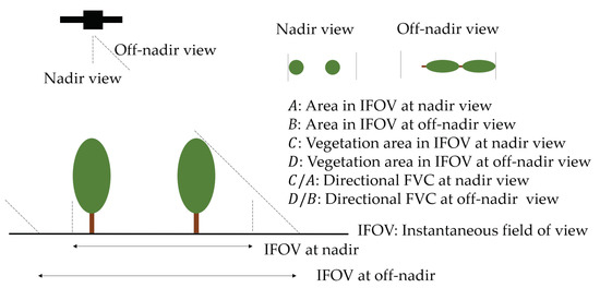
Figure 1.
Illustration of the viewing angle dependency of the directional FVC. The directional FVC at nadir-view corresponds to the general definition of the FVC.
In the present study, reflectances are expressed by a sum of the vegetation and nonvegetation reflectances showing surface anisotropy with the directional FVC for a fraction of vegetation reflectances:
where is a modeled reflectance for ; i corresponds to the direction of the solar angle specific to the solar zenith and azimuth angles; j corresponds to the direction of the sensor (viewing) angle specific to the sensor zenith and azimuth angle; is the directional FVC; is the vegetation reflectance; is the nonvegetation reflectance (subscripts v and s denote vegetation and nonvegetation (soil), respectively); and vary with the viewing angle and with the sun angle condition that changes sunlit and shaded parts over vegetation canopy and nonvegetation surfaces. A spectrum that consists of multiple bands (two bands in the present study) of vegetation or nonvegetation reflectances is referred to as an endmember spectrum. The endmember spectra and the directional FVC are sensitive to the structure of the canopy and to the density and spatial distributions of canopy stands when the angular condition varies [32,33,34], which is, however, not explicitly expressed in Equation (1).
The directional FVC for a pixel can be derived by minimizing the Euclidean distance between modeled and target spectra [25], where endmember spectra for a scene are extracted prior to the minimization. Similarly, the directional FVC can be derived by minimizing differences between NDVIs from modeled and target spectra with endmember spectra for the scene [35,36]. In a previous study, the latter approach was used to derive the FVC for spatially uniform atmospheric conditions [23]. The directional FVC specific to viewing directions can be expressed by
and
where and are the TOA, partially atmosphere-corrected or fully atmosphere-corrected reflectances of the target spectrum and subscripts r and n correspond to red and NIR bands, respectively; is the TOA, partially atmosphere-corrected or fully atmosphere-corrected endmember spectra for vegetation and nonvegetation ( corresponds to v or s). The terms and are functions of the target NDVI and the second- and higher-order interaction terms between the atmosphere and surfaces. The details of Equation (2) are shown in Appendix A.
The values of and are equal to zero when the reflectances are atmospherically corrected. The values of and for TOA-level or partially atmosphere-corrected reflectances are expected to be close to zero because the individual terms of the red and NIR bands in and tend to cancel out [23]. Thus, the expression form of the equation for directional FVC as a function of TOA or partially atmosphere-corrected reflectances is identical to that as a function of fully atmosphere-corrected reflectances when . Note that, in general, the value of the directional FVC tends to be sensitive to atmospheric correction levels unless correct endmember spectra are chosen for a pixel such that the Euclidean distance between the modeled and target spectra becomes zero.
3. Derivation of the NDVI Transformation Equation
Directional FVCs of two sensors are defined, and then the FVCs are used to relate NDVIs of different sensors. The resultant NDVI transformation equation is a function of the endmember spectra for two sensors.
Two sensor types are defined: an original sensor that is a sensor-to-be-transformed, and a destination sensor. The directional FVC for each sensor is expressed by
where the subscript in Equation (10) and in the following equations corresponds to a (sensor-a, original sensor) or b (sensor-b, destination sensor).
The FVC is used as a parameter to relate the NDVI of two sensors ( and ). The following equation with an error term () is assumed:
where represents an error included in with reference to and is sensitive to the structure of the canopy and to the density and spatial distribution of the canopy stands.
An NDVI transformation equation describing the inter-sensor NDVI relationship is derived using Equations (5)–(11), in which geometric variables ( and ) are omitted for brevity:
where
and
A flow diagram of the derivation is illustrated in Figure 2.
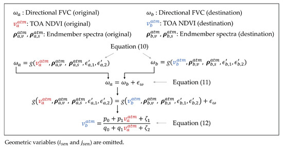
Figure 2.
Illustration of the steps in the derivation of the NDVI transformation equation.
4. Transformation Algorithm
4.1. Overview of the Algorithm
A basic NDVI transformation algorithm is illustrated in Figure 3. First, endmember spectra of the original GEO sensor ( and ) are computed using the automated algorithm of endmember computation which is described in Section 4.2; the NDVI of the original sensor () can also be computed (step 1). Second, endmember spectra of the destination LEO sensor ( and ) are computed using the same endmember algorithm (step 2). Finally, endmember spectra for each sensor and the GEO NDVI are used to estimate the LEO-compatible NDVI () (step 3).
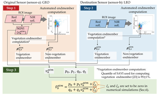
Figure 3.
Schematic of a basic algorithm for the NDVI transformation equation.
The NDVI computed using LEO data (), which is not shown in Figure 3, can be used to evaluate the transformed NDVI here denoted by to distinguish it from the NDVI denoted by . In our numerical demonstration described in Section 6, this evaluation is carried out with the values of and set to zero. Real applications of the time-series analysis using the method are discussed in Section 8.2.
4.2. Automated Endmember Computation
Vegetation and nonvegetation endmember spectra for original and destination sensors are necessary to transform the NDVI using Equation (12). For this transformation, the present study requires a single set of endmember spectra for each sensor scene. A representative approach to endmember extraction is to use vertices of scatter plots for the target area over the reflectance space [37] or feature space [38]. In a previous study, a similar idea was used for computing vegetation and nonvegetation endmember spectra using red–NIR reflectance scatter-plot information [23]; this approach is also used in the present study. Instead of finding vertices, the algorithm automatically finds a point along the left side boundary of the red and NIR reflectance scatter plot for computing the vegetation endmember spectrum and a point along the right side boundary (soil line) for computing the nonvegetation endmember spectrum. Note that the endmember spectra for the NDVI transformation equations are merely parameter vectors and need not be pure [23], which is discussed in Section 8.2.
5. Test Sites and Materials for Numerical Demonstration
5.1. Test Sites
Land surfaces at middle latitude where the viewing zenith angle of AHI shows middle values—specifically, approximately 40–50°—were explored. Among these land surfaces, that of Japan (Figure 4a) was identified as suitable for our demonstration for the following reasons: (1) Several climatic zones are included because Japan is located in a transitional zone between sub-boreal to sub-tropical [39], and (2) large variations of reflectances along seasons are expected because of Japan’s mountainous topography and higher solar zenith angle at LEO (Aqua) overpass time in winter, which is a consequence of Japan being located at true north of the sub-satellite point of AHI. The solar zenith angle variation in our regions of interest (ROIs) was approximately 19–64° (area-averaged value), which likely caused variations of the areas for shaded parts. These characteristics make our demonstrations more stringent. Descriptions of the ROIs used in the present study are introduced in Section 5.3.
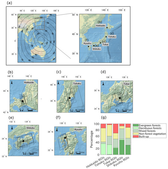
Figure 4.
(a) Location of Japan and the centers of the five test sites. Contour lines in the left panel depict the viewing zenith angle of AHI; (b) the Hokkaido site, where the ROIs are depicted by dotted lines; (c) the Tohoku site; (d) the Tokai site; (e) the Shikoku site; (f) the Kyushu site; and (g) the averages of land cover percentage in the ROIs for each site, as created on the basis of the MODIS land cover products.
The maps in Figure 4b–f show the five test sites: Hokkaido, Tohoku, Tokai, Shikoku, and Kyushu (from north to south, 31–45° N, 129–143° E). Dotted rectangles or parallelograms in the maps are polygons for the ROI, which vary with the date of observation. The geographic coordinates for each site used for exploring data (the center of each site) and the viewing angles of AHI for the coordinates are summarized in Table 1. The Hokkaido and Tohoku ROIs are located primarily in a cool temperate zone; the other three ROI sites are dominated by a warm temperate zone. The compositions of the land cover in the ROIs differ across sites, as shown in Figure 4g, which was created using the MODIS land cover product (MCD12Q1C) [40]. Evergreen forests in Figure 4g include, for example, coniferous species such as Japanese cedar (Cryptomeria japonica) and Hinoki cypress (Chamaecyparis obtusa) and broadleaf species such as Japanese chinquapin (Castanopsis sieboldii) and evergreen oaks (e.g., Quercus glauca). Deciduous forests include deciduous oaks (e.g., Quercus serrata and Quercus crispula) and Japanese beech (e.g., Fagus crenata), among others [39,41,42]. Nonforest vegetation in Figure 4g includes rice paddy, crop, and grasslands [43].

Table 1.
Geographic coordinates of each site center, and the AHI viewing angles for each coordinate in decimal degrees [23].
5.2. Satellite Data
The Himawari 8 is located at 140.7° E, and the AHI onboard the Himawari 8 observes 16 bands from the visible to the infrared region. The AHI performs a full disk observation with 10 min intervals. The Center for Environmental Remote Sensing (CEReS) at Chiba University distributes Himawari 8 AHI data, which are gridded over the geographic coordinates [44,45]. Red-band data (band 3) are gridded with a 0.005° interval, and blue, green, and near-infrared (NIR)-band data (bands 1, 2, and 4, respectively) are gridded with a 0.01° interval. These data were downloaded from the CEReS ftp site (ftp://hmwr829gr.cr.chiba-u.ac.jp/, (accessed on 27 August 2021)). The AHI TOA reflectances for each band were computed using the apparent reflectance values, solar zenith angle, and the sun-to-Earth distance [23]. The AHI red band (band 3) reflectances were aggregated arithmetically to obtain 0.01° data.
The MODIS onboard Aqua flies an afternoon orbit, and its Equator crossing time is 1:30 p.m. The Collection 6.1 Calibrated Radiances, the Daily L1B Swath 1 km (MYD021KM) [46], and the corresponding Geolocation (MYD03) [47] were downloaded from the Level 1 and Atmosphere Archive and Distribution System (LAADS) Distributed Active Archive Center (DAAC) website (https://ladsweb.modaps.eosdis.nasa.gov/, (accessed on 27 August 2021)). Note that the MODIS data were limited to data including the test sites observed from the near-nadir direction. The MODIS TOA reflectances for each band were computed using scaled integer values, calibration coefficients, and the solar zenith angle.
5.3. Partial Scene Pair for ROIs
The ROI data for the five sites are the same as those used in [23] except that the AHI data were converted from data from the National Institute of Information and Communications Technology (NICT) Science Cloud into CEReS gridded data because the gridded data contain fewer geolocation errors [45]. Nearly coincident and collocated AHI and MODIS data were used, and the date range of the data spanned between July 2015 and December 2018. The number of pairs of AHI and MODIS partial scenes for the Hokkaido, Tohoku, Tokai, Shikoku, and Kyushu sites were 10, 12, 14, 16, and 12, respectively.
The ROIs were extracted to have as many pixels as possible from km2 areas centered on the coordinates for each site (Table 1); during the extraction, pixels corresponding to a MODIS zenith viewing angle larger than 10° or cloudy pixels were excluded. The number of pixels used for analysis was greater than 1000 for every partial scene. The coordinate information for all of the ROIs is provided in the supplementary materials in [23].
6. Numerical Demonstration Procedure
To numerically demonstrate the NDVI transformation method, we evaluated differences between MODIS NDVI at near-nadir view and MODIS-compatible AHI NDVI at near-nadir view (transformed AHI NDVI), where the MODIS NDVI was used as a reference.
For the five test sites shown in Section 5, the variables and in Equation (12) were assumed to be zero in the numerical experiments. The reasoning for this assumption is explained as follows. Similar frequency distributions of the directional FVCs ( in Equation (10)) from the TOA AHI (off-nadir view) and TOA Aqua MODIS (near-nadir view) data were observed at our test sites [23]. Although a few scenes exist in which the FVCs show a strong viewing angle dependency, the assumption that in and are zero during the NDVI transformation is mostly reasonable. In addition, and in and were set to be zero because and for each sensor would be close to zero. These assumptions enable us to omit and from the NDVI transformation equation.
Scene-level and pixel-by-pixel comparisons of NDVIs were conducted. MODIS and AHI pixels that include water bodies identified by the land/sea mask in the MYD03 product were excluded from our analysis of the NDVI differences after endmember computations [23]. In the scene-level comparisons, differences between area-averaged values of AHI NDVI or transformed AHI NDVI and MODIS NDVI were computed for all partial scenes. Their averages for each site, denoted by m, were computed as follows:
and
where is the average of the differences between the area-averaged AHI and MODIS NDVIs for site m; is the average of the differences between the area-averaged transformed AHI and MODIS NDVIs; , , and are the AHI, MODIS, and transformed AHI NDVIs for the n-th pixel of the k-th date at site m, respectively; is the number of the date relying on the site; and and are the number of pixels relying on the date and site for the AHI and MODIS, respectively.
In the pixel-by-pixel comparison, NDVIs obtained at 0.01° or 1 km spatial resolution were aggregated at pixels using the arithmetic mean for mitigating the effects of geolocation errors and pixel size differences. Each pixel of an aggregated MODIS NDVI was paired with an aggregated original or transformed AHI NDVI using a nearest-neighbor algorithm. Linear regression analysis was conducted to evaluate the results obtained using these NDVIs for each partial scene. In addition, for each site, the aggregated MODIS NDVI for all dates were combined to generate a single MODIS NDVI dataset. Similarly, a single NDVI dataset of AHI or transformed AHI at each site was generated. Note that each pixel in the AHI or transformed AHI dataset is paired with one of the pixels in the MODIS NDVI dataset. The AHI, MODIS, and transformed AHI NDVI of the ℓ-th pixel for the dataset of site m were denoted by , , and , respectively. The differences between and () and between and () were computed for each pixel:
The mean of the absolute values for Equations (26) and (27) in each site, referred to as the mean absolute difference (MAD) of NDVI, and the standard deviation (SD) of Equations (26) and (27) in each site were also computed. In the following equations, the subscript corresponds to either the original AHI () or the transformed AHI (), and we have
and
where is the MAD for site m and is the SD for site m. Parameter is the total number of the pixel pair dependent on site m.
7. Results
7.1. Scene-Level Evaluations of NDVI Transformation
Results for relative frequency distributions of TOA NDVIs for AHI and MODIS are shown in Figure 5 and Figure 6. Figure 5 corresponds to the “best date” for each site, where the absolute value of the averaged AHI (transformed) minus the MODIS NDVIs was minimal among all dates. By contrast, Figure 6 corresponds to the “worst date”, which provides the maximal absolute value of the averaged AHI minus the MODIS NDVIs. The left column in Figure 5 shows similar distributions of the AHI and MODIS NDVI, although slight differences are observed, especially at higher NDVI values. Thus, the MODIS NDVI was slightly higher than the AHI NDVI. The right column in Figure 5 shows a much more similar distribution of the AHI (transformed) and MODIS NDVI, indicating successful transformations of the NDVI. The left column in Figure 6 shows the same trend as the left column in Figure 5; however, the right column in Figure 6 shows slight under- and over-corrections (e.g., Figure 6d,f), which are not observed in the right columns in Figure 5.
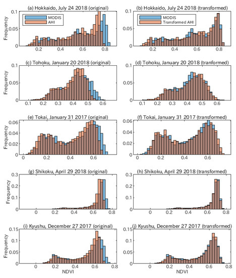
Figure 5.
Relative frequency distributions of the NDVI for the AHI and MODIS (left column) and the transformed AHI and MODIS (right column) for best date. Each row of figures corresponds to a site.
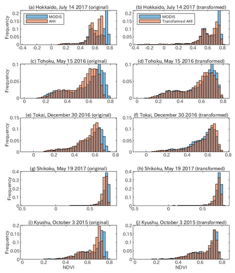
Figure 6.
Relative frequency distributions for the worst date, where the absolute value of the averaged transformed AHI NDVI minus the averaged MODIS NDVI was maximal, at each site.
The mean of the averaged AHI or transformed AHI minus MODIS NDVIs for each site ( and ) is summarized in Table 2. The original AHI NDVIs were approximately 0.02 smaller than the MODIS in NDVI units. Biases between the transformed AHI and MODIS NDVIs were much smaller (the absolute value of the mean was smaller than 0.01).
Table 2.
Mean of the averaged AHI or the transformed AHI minus MODIS NDVIs for the five sites ( and ).
Figure 7 shows the averages and standard deviations of the coefficients of the NDVI transformation equation (Equations (13)–(16)) for each site. The averaged values are negative values and fall between and 0 (Figure 7a). The Hokkaido and Shikoku sites show larger negative values. The averaged and values are approximately 0.4–0.7 and 0.4–0.5, respectively. The averaged for Shikoku is higher than those of the other sites. This coefficient reflects nonlinear effects of the NDVI transformation equation and simply minus . The for Shikoku is higher than the corresponding in almost all cases, indicating that inter-sensor relationships between the NDVIs for Shikoku could be slightly more nonlinear than those for the other sites.
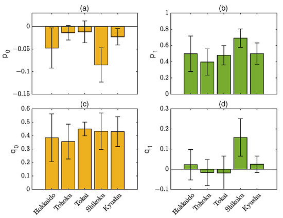
Figure 7.
Averages for the four coefficients in the NDVI transformation equation (, , , and ) for the five test sites. (a–d) correspond to , , , and , respectively. The error bars correspond to the standard deviation.
7.2. Pixel-by-Pixel Evaluations of the NDVI Transformation
Aggregated NDVIs were used for pixel-by-pixel evaluations. Figure 8 shows the spatial distribution of the NDVI differences between sensors for the partial scene of the Shikoku site on 13 April 2018. Figure 8a shows the spatial distribution of the aggregated MODIS NDVI. Negative biases could be identified in numerous parts in the original NDVI differences (Figure 8b). The large errors are attributable to sensor noises and to random errors caused by remaining relative geolocation differences, atmospheric and cloud contamination differences due to differences in the observation times (within approximately 5 min), and unidentified error sources. Overall negative errors were reduced or turned into small positive errors after the transformations (Figure 8c).
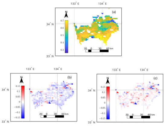
Figure 8.
Maps of aggregated NDVI and their differences between AHI and MODIS for the data corresponding to Shikoku region on 13 April 2018: (a) MODIS NDVI, (b) AHI NDVI minus MODIS NDVI, and (c) transformed AHI NDVI minus MODIS NDVI.
Density scatter plots of AHI NDVI vs. MODIS NDVI for the data (Shikoku, 13 April 2018) are shown in Figure 9a, and plots of the transformed AHI NDVI vs. MODIS NDVI are shown in Figure 9b. These plots indicate that the AHI NDVI approached the one-to-one line after the transformations, indicating that the biases were mitigated. The results for other data for Shikoku and other sites typically showed the same trend, although substantial biases of the NDVI were observed in specific pixels after the transformations. Figure 9c,d show the results for Hokkaido on 14 July 2017. After the transformation, negative biases were observed at certain points where the MODIS NDVIs were less than approximately 0.5 (Figure 9d). These negative biases might be attributable to the fact that directional FVCs from two sensors showed biases over areas that included sparsely distributed vegetation. In such areas, the light interception by the vegetation canopy may have sharply increased with increasing viewing zenith angle, thereby increasing the NIR transmittances and reflectances of vegetation as well as the top-of-canopy reflectances. The increase in the AHI NIR reflectances subsequently resulted in FVC biases between the sensors [23]. The FVC biases would have propagated into the transformed AHI NDVI in such cases.
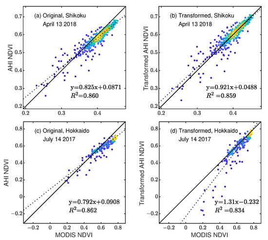
Figure 9.
Density scatter plot of the aggregated NDVIs: (a) AHI vs. MODIS NDVI for Shikoku, 13 April 2018; (b) transformed AHI vs. MODIS NDVI for Shikoku, 13 April 2018; (c) AHI vs. MODIS NDVI for Hokkaido, 14 July 2017; and (d) transformed AHI vs. MODIS NDVI for Hokkaido, 14 July 2017.
Finally, Table 3 summarizes the MAD ( and ) and the SD ( and ). The MAD decreased after the transformations, whereas the SD slightly increased. The relatively large increase in the SD in Hokkaido is attributable to the directional FVC biases between the sensors.
Table 3.
The MAD between the AHI or transformed AHI NDVI and MODIS NDVI ( and ), and the SD for the NDVI differences ( and ) obtained using NDVI data for pixel-by-pixel comparisons.
8. Discussion
8.1. Comparison of the Developed Method with Other Methods
Previous studies regarding vegetation index (VI) inter-comparisons between GEO and LEO sensors have typically applied BRDF correction/adjustment of reflectances to mitigate the effects of surface anisotropy [15,16,18,48]. Two sensors’ VIs derived using the corrected/adjusted reflectances were then used to compare phenologically significant transition dates [11]. In the present study, our intention was to reduce the absolute NDVI differences between sensors. A few studies quantitatively investigated the absolute NDVI differences using BRDF-adjusted reflectances (e.g., [16,48]); for example, Tran et al. [16] reported that mean absolute differences between atmospherically corrected, near-solar-noon AHI NDVI and atmospherically corrected and BRDF-adjusted MODIS NDVI (adjusted to solar noon and an oblique AHI viewing angle) was only 0.018–0.030 over Australian grassland/pasture sites. The remaining errors between the VIs are likely attributable to discrepancies in pixel footprints, geolocation accuracy, cloud mask methods, atmospheric correction methods, SRFs, and calibration uncertainties. The method developed in the present work is distinct from the common approaches using the BRDF method. In particular, our method is capable of standardizing the GEO NDVI to the near-nadir viewing direction and mitigating the effects of differences in the SRFs.
In the present study, we used the directional FVC as a parameter to derive the NDVI transformation equation on the basis of the equivalence of the FVCs between sensors with the error term. Similar approaches assuming the equivalence of physical parameters for deriving inter-sensor VIs or reflectances equations have been reported [22,49,50,51,52,53,54]. To quantitatively estimate the coefficients of the equations, which are functions of physically meaningful parameters, nonlinear regression was successfully applied for global applications [52]. On the contrary, coefficients of NDVI transformation equations could be obtained without using regression analysis. For example, atmospheric parameters and hyperspectral profile of surfaces [22] or pixel-by-pixel minimum and maximum NDVIs from smoothed NDVI products [55] were prepared and used to compute the coefficients for NDVI conversion equations. Compared to these, our method does not require any prior information, and coefficients of the transformation equation could be automatically computed using reflectance data.
8.2. Benefits and Limitations of the Developed Method
The method developed in the present study can not only be used to geometrically and spectrally transform the NDVI but may be less sensitive to several biases included in the data. This reduced sensitivity is attributable to the endmember spectra used to compute the coefficients of the transformation equation and the target spectra both being influenced by sensor-dependent biases (e.g., biases in gain coefficients for radiometric calibration) and, thus, directional FVCs tend to be sensor-independent, leading to correct transformations of the NDVI. The advantage of using such “image endmembers” for reducing the effects of biases included in the data has also been reported in studies for spectral mixture analysis [56] as well as relative radiometric normalization between different sensors [57].
The NDVI transformation reduced biases between NDVIs in our results; however, the variability of the NDVI differences remained or slightly increased, possibly because of the viewing angle dependency of the FVC and errors that cannot be corrected in the transformation. The errors likely arise from observation time differences between the sensors (within approximately 5 min [23]) causing cloud and atmospheric condition differences, pixel footprint differences, geolocation errors, and intrinsic sensor noise. Thus, consideration of the directional FVC biases, i.e., in the transformation, and improvements in the data quality (e.g., sensor noise and geolocation errors) would further reduce the variability of the NDVI differences after the NDVI transformation [51]. Additionally, to mitigate the effects of differences in FVC as a function of direction in numerical evaluations of the method, reference data can be chosen that utilize MODIS data obtained at similar viewing zenith and relative-azimuthal angles to AHI [17].
In real applications of the transformation algorithm, finding pure endmember spectra from coarse spatial resolution (1 km) data is challenging [23]. Even though reflectance spectra used for endmembers were not pure, we expect that the NDVI transformation using Equation (12) functions properly if the FVC values computed using those endmembers are known to be equivalent between sensors or the correct value is known. Meanwhile, the effects of non-purity for endmember spectra obtained from 1 km resolution data on the transformation should be quantitatively evaluated using high spatial resolution (e.g., ≤10 m) data. This evaluation would, however, require considerable efforts for data processing and should be conducted in future works.
Note that the NDVI transformation for full-disk scale is not available using a single implementation of the method because atmospheric contamination should be as spatially uniform as possible and because variations of the sun and viewing angles should be as small as possible in the data for processing. Therefore, regional-scale NDVI transformation with moving-window approaches would be required to cover broader areas.
Although our proposed method still faces several unresolved problems, it can be used to predict near-real-time LEO-compatible GEO NDVI toward time-series vegetation analysis for a specific region. In this application, regional- or full-disk-scale reference sensor (LEO) reflectances with a certain temporal resolution (e.g., 8-day) should be prepared and used to predict the endmember spectra of a destination sensor for the time when a GEO system makes an observation. In addition, GEO reflectances observed in various solar zenith and azimuth angles should be normalized prior to or during the NDVI transformations.
9. Conclusions
In this study, we derived a GEO-to-LEO NDVI transformation equation based on a linear mixture model of anisotropic vegetation and nonvegetation endmember spectra. Using the derived equation, we developed an NDVI transformation method in which endmember spectra from each set of sensor data are computed independently and subsequently combined to compute the coefficients of the transformation equation. The proposed method could reduce the effects of surface anisotropy caused by viewing angle differences and SRF differences at the scene level. Moreover, the NDVI transformation is insensitive to calibration biases because the endmember spectra are computed using data. Notably, our method does not require regression analysis for the NDVI transformation because the endmember spectra used in the coefficients of the transformation equations are independently extracted from each sensor dataset.
Numerical demonstrations of the method were conducted using Himawari 8 AHI at off-nadir-view and Aqua MODIS at near-nadir-view data in middle latitude test sites, where the directional FVCs of the sites were reported to be nearly identical except for a few cases. The results showed that, compared with the original AHI NDVI, the transformed AHI NDVI was closer to the MODIS NDVI. The magnitudes of the averaged NDVI biases between the AHI and MODIS were reduced from 0.016–0.026 to <0.01 after the NDVI transformation was applied to the AHI NDVI. However, biases between FVCs from GEO and LEO sensors, which were caused by the viewing angle dependency of the directional FVC, may have added errors during the NDVI transformation. We expect that inclusions of the directional FVC biases would reduce the transformation errors.
The developed method is universally applicable to NDVI transformation among distinct sensors. Thus, the method can be used for not only GEO and LEO sensors but also, for example, LEO sensors on different platforms.
In future studies, further evaluations of the NDVI transformation using data obtained using various viewing angles and land-cover types are necessary. In addition, although this study used TOA reflectances for evaluation and demonstration purposes, the proposed method is capable of transforming partially or fully atmosphere-corrected NDVIs, which should be evaluated in a separate study. Furthermore, NDVI transformation across different atmospheric conditions (e.g., TOA to bottom-of-atmosphere) should be investigated and evaluated to explore the possibility of avoiding atmospheric corrections of original sensor data. Finally, the proposed method should be expanded to be capable of near-real-time GEO-to-LEO NDVI transformation across broader spatial scales. This would make it possible to obtain the spatial information of vegetation index time series with high temporal resolution and NDVI compatibility between GEO and LEO sensors.
Author Contributions
Conceptualization, K.O. and H.Y.; methodology, K.O. and H.Y.; software, K.O.; validation, K.O., M.M., H.Y. and K.T.; formal analysis, K.O.; investigation, K.O.; resources, K.O.; data curation, K.O.; writing—original draft preparation, K.O.; writing—review and editing, K.O., H.Y., K.T. and M.M.; visualization, K.O.; supervision, K.O.; project administration, K.O.; funding acquisition, K.O. and H.Y. All authors have read and agreed to the published version of the manuscript.
Funding
This research was funded by JSPS KAKENHI Grand Numbers JP20K12259, JP20K20487, JP20KK0237.
Informed Consent Statement
Not applicable.
Data Availability Statement
Himawari 8 AHI data were downloaded from CEReS, Chiba University (ftp://hmwr829gr.cr.chiba-u.ac.jp/, (accessed on 27 August 2021)). Aqua MODIS calibrated radiances and geolocation data (MYD021KM and MYD03) as well as MODIS land cover product (MCD12Q1C) were downloaded from the LAADS DAAC (https://ladsweb.modaps.eosdis.nasa.gov/, (accessed on 27 August 2021)).
Acknowledgments
Authors are grateful to CEReS, Chiba University for distributing the Himawari 8 AHI gridded data. Appreciation is extended to the NASA Goddard Space Flight Center for distributing Aqua MODIS data (MYD021KM, MYD03) as well as MODIS land cover product (MCD12Q1C).
Conflicts of Interest
The authors declare no conflict of interest.
Appendix A. Description of Directional FVC
The description of directional FVC ( in Equation (2)) is introduced in this section. This equation was derived in [23] and is written here again as
where
and endmember reflectances () are expressed by
where is atmospheric reflectances, and are the downward and upward atmospheric transmittances, and is the spherical albedo of the atmosphere. Note that and are variables that can be obtained or computed from observation data.
Parameters and in Equation (A1) are expressed as
where
Parameter is a function of the second- and higher-order interaction terms between the surface and atmosphere, and is the interaction terms between the surface of an endmember and the atmosphere. For the fully atmosphere-corrected reflectances, and are zero and and are unity; thus, and become zero.
References
- Myneni, R.B.; Keeling, C.D.; Tucker, C.J.; Asrar, G.; Nemani, R.R. Increased plant growth in the northern high latitudes from 1981 to 1991. Nature 1997, 386, 698–702. [Google Scholar] [CrossRef]
- Fensholt, R.; Sandholt, I.; Rasmussen, M.S. Evaluation of MODIS LAI, fAPAR and the relation between fAPAR and NDVI in a semi-arid environment using in situ measurements. Remote Sens. Environ. 2004, 91, 490–507. [Google Scholar] [CrossRef]
- Gitelson, A.A. Remote estimation of fraction of radiation absorbed by photosynthetically active vegetation: Generic algorithm for maize and soybean. Remote Sens. Lett. 2019, 10, 283–291. [Google Scholar] [CrossRef]
- Tucker, C.J.; Pinzon, J.E.; Brown, M.E.; Slayback, D.A.; Pak, E.W.; Mahoney, R.; Vermote, E.F.; Saleous, N.E. An extended AVHRR 8-km NDVI dataset compatible with MODIS and SPOT vegetation NDVI data. Int. J. Remote Sens. 2005, 26, 4485–4498. [Google Scholar] [CrossRef]
- Sobrino, J.A.; Julien, Y. Global trends in NDVI-derived parameters obtained from GIMMS data. Int. J. Remote Sens. 2011, 32, 4267–4279. [Google Scholar] [CrossRef]
- Fensholt, R.; Proud, S.R. Evaluation of Earth Observation based global long term vegetation trends—Comparing GIMMS and MODIS global NDVI time series. Remote Sens. Environ. 2012, 119, 131–147. [Google Scholar] [CrossRef]
- Zhang, X.; Liu, L.; Yan, D. Comparisons of global land surface seasonality and phenology derived from AVHRR, MODIS, and VIIRS data. J. Geophys. Res. Biogeo. 2017, 122, 1506–1525. [Google Scholar] [CrossRef]
- Wang, W.; Li, S.; Hashimoto, H.; Takenaka, H.; Higuchi, A.; Kalluri, S.; Nemani, R. An Introduction to the Geostationary-NASA Earth Exchange (GeoNEX) Products: 1. Top-of-Atmosphere Reflectance and Brightness Temperature. Remote Sens. 2020, 12, 1267. [Google Scholar] [CrossRef]
- Bessho, K.; Date, K.; Hayashi, M.; Ikeda, A.; Imai, T.; Inoue, H.; Kumagai, Y.; Miyakawa, T.; Murata, H.; Ohno, T.; et al. An Introduction to Himawari-8/9—Japan’s New-Generation Geostationary Meteorological Satellites. J. Meteorol. Soc. Jpn. Ser. II 2016, 94, 151–183. [Google Scholar] [CrossRef]
- Schmit, T.J.; Griffith, P.; Gunshor, M.M.; Daniels, J.M.; Goodman, S.J.; Lebair, W.J. A Closer Look at the ABI on the GOES-R Series. Bull. Am. Meteorol. Soc. 2017, 98, 681–698. [Google Scholar] [CrossRef]
- Yan, D.; Zhang, X.; Nagai, S.; Yu, Y.; Akitsu, T.; Nasahara, K.N.; Ide, R.; Maeda, T. Evaluating land surface phenology from the Advanced Himawari Imager using observations from MODIS and the Phenological Eyes Network. Int. J. Appl. Earth Obs. Geoinf. 2019, 79, 71–83. [Google Scholar] [CrossRef]
- Miura, T.; Nagai, S.; Takeuchi, M.; Ichii, K.; Yoshioka, H. Improved Characterisation of Vegetation and Land Surface Seasonal Dynamics in Central Japan with Himawari-8 Hypertemporal Data. Sci. Rep. 2019, 9, 15692. [Google Scholar] [CrossRef]
- Hashimoto, H.; Wang, W.; Dungan, J.L.; Li, S.; Michaelis, A.R.; Takenaka, H.; Higuchi, A.; Myneni, R.B.; Nemani, R.R. New generation geostationary satellite observations support seasonality in greenness of the Amazon evergreen forests. Nat. Commun. 2021, 12, 684. [Google Scholar] [CrossRef]
- Fensholt, R.; Sandholt, I.; Stisen, S.; Tucker, C. Analysing NDVI for the African continent using the geostationary meteosat second generation SEVIRI sensor. Remote Sens. Environ. 2006, 101, 212–229. [Google Scholar] [CrossRef]
- Yeom, J.M.; Kim, H.O. Feasibility of using Geostationary Ocean Colour Imager (GOCI) data for land applications after atmospheric correction and bidirectional reflectance distribution function modelling. Int. J. Remote Sens. 2013, 34, 7329–7339. [Google Scholar] [CrossRef]
- Tran, N.N.; Huete, A.; Nguyen, H.; Grant, I.; Miura, T.; Ma, X.; Lyapustin, A.; Wang, Y.; Ebert, E. Seasonal Comparisons of Himawari-8 AHI and MODIS Vegetation Indices over Latitudinal Australian Grassland Sites. Remote Sens. 2020, 12, 2494. [Google Scholar] [CrossRef]
- Adachi, Y.; Kikuchi, R.; Obata, K.; Yoshioka, H. Relative Azimuthal-Angle Matching (RAM): A Screening Method for GEO-LEO Reflectance Comparison in Middle Latitude Forests. Remote Sens. 2019, 11, 1095. [Google Scholar] [CrossRef]
- Proud, S.R.; Zhang, Q.; Schaaf, C.; Fensholt, R.; Rasmussen, M.O.; Shisanya, C.; Mutero, W.; Mbow, C.; Anyamba, A.; Pak, E.; et al. The Normalization of Surface Anisotropy Effects Present in SEVIRI Reflectances by Using the MODIS BRDF Method. IEEE Trans. Geosci. Remote Sens. 2014, 52, 6026–6039. [Google Scholar] [CrossRef]
- Fan, X.; Liu, Y. Multisensor Normalized Difference Vegetation Index Intercalibration: A Comprehensive Overview of the Causes of and Solutions for Multisensor Differences. IEEE Trans. Geosci. Remote Sens. Mag. 2018, 6, 23–45. [Google Scholar] [CrossRef]
- Qin, Y.; McVicar, T.R. Spectral band unification and inter-calibration of Himawari AHI with MODIS and VIIRS: Constructing virtual dual-view remote sensors from geostationary and low-Earth-orbiting sensors. Remote Sens. Environ. 2018, 209, 540–550. [Google Scholar] [CrossRef]
- Chander, G.; Hewison, T.J.; Fox, N.; Wu, X.; Xiong, X.; Blackwell, W.J. Overview of Intercalibration of Satellite Instruments. IEEE Trans. Geosci. Remote Sens. 2013, 51, 1056–1080. [Google Scholar] [CrossRef]
- Fan, X.; Liu, Y. A Generalized Model for Intersensor NDVI Calibration and Its Comparison With Regression Approaches. IEEE Trans. Geosci. Remote Sens. 2017, 55, 1842–1852. [Google Scholar] [CrossRef]
- Obata, K.; Yoshioka, H. A Simple Algorithm for Deriving an NDVI-Based Index Compatible between GEO and LEO Sensors: Capabilities and Limitations in Japan. Remote Sens. 2020, 12, 2417. [Google Scholar] [CrossRef]
- Gao, L.; Wang, X.; Johnson, B.A.; Tian, Q.; Wang, Y.; Verrelst, J.; Mu, X.; Gu, X. Remote sensing algorithms for estimation of fractional vegetation cover using pure vegetation index values: A review. ISPRS J. Photogramm. Remote Sens. 2020, 159, 364–377. [Google Scholar] [CrossRef]
- Xiao, J.; Moody, A. A comparison of methods for estimating fractional green vegetation cover within a desert-to-upland transition zone in central New Mexico, USA. Remote Sens. Environ. 2005, 98, 237–250. [Google Scholar] [CrossRef]
- Baret, F.; Hagolle, O.; Geiger, B.; Bicheron, P.; Miras, B.; Huc, M.; Berthelot, B.; Niño, F.; Weiss, M.; Samain, O.; et al. LAI, fAPAR and fCover CYCLOPES global products derived from VEGETATION: Part 1: Principles of the algorithm. Remote Sens. Environ. 2007, 110, 275–286. [Google Scholar] [CrossRef]
- Liu, D.; Yang, L.; Jia, K.; Liang, S.; Xiao, Z.; Wei, X.; Yao, Y.; Xia, M.; Li, Y. Global Fractional Vegetation Cover Estimation Algorithm for VIIRS Reflectance Data Based on Machine Learning Methods. Remote Sens. 2018, 10, 1648. [Google Scholar] [CrossRef]
- Liu, J.; Melloh, R.A.; Woodcock, C.E.; Davis, R.E.; Ochs, E.S. The effect of viewing geometry and topography on viewable gap fractions through forest canopies. Hydrol. Process. 2004, 18, 3595–3607. [Google Scholar] [CrossRef]
- Liu, J.; Woodcock, C.E.; Melloh, R.A.; Davis, R.E.; McKenzie, C.; Painter, T.H. Modeling the View Angle Dependence of Gap Fractions in Forest Canopies: Implications for Mapping Fractional Snow Cover Using Optical Remote Sensing. J. Hydrometeorol. 2008, 9, 1005–1019. [Google Scholar] [CrossRef]
- Song, W.; Mu, X.; Ruan, G.; Gao, Z.; Li, L.; Yan, G. Estimating fractional vegetation cover and the vegetation index of bare soil and highly dense vegetation with a physically based method. Int. J. Appl. Earth Obs. Geoinf. 2017, 58, 168–176. [Google Scholar] [CrossRef]
- Mu, X.; Song, W.; Gao, Z.; McVicar, T.R.; Donohue, R.J.; Yan, G. Fractional vegetation cover estimation by using multi-angle vegetation index. Remote Sens. Environ. 2018, 216, 44–56. [Google Scholar] [CrossRef]
- Li, X.; Strahler, A.H. Geometric-Optical Modeling of a Conifer Forest Canopy. IEEE Trans. Geosci. Remote Sens. 1985, 23, 705–721. [Google Scholar] [CrossRef]
- Li, C.; Song, J.; Wang, J. Modifying Geometric-Optical Bidirectional Reflectance Model for Direct Inversion of Forest Canopy Leaf Area Index. Remote Sens. 2015, 7, 11083–11104. [Google Scholar] [CrossRef]
- Pisek, J.; Rautiainen, M.; Nikopensius, M.; Raabe, K. Estimation of seasonal dynamics of understory NDVI in northern forests using MODIS BRDF data: Semi-empirical versus physically-based approach. Remote Sens. Environ. 2015, 163, 42–47. [Google Scholar] [CrossRef]
- Verstraete, M.; Pinty, B. The potential contribution of satellite remote-sensing to the understanding of arid lands processes. In Vegetation and Climate Interactions in Semi-Arid Regions; Henderson-Sellers, A., Pitman, A., Eds.; Springer: Dordrecht, The Netherlands, 1991; pp. 59–72. [Google Scholar]
- Obata, K.; Yoshioka, H. Inter-Algorithm Relationships for the Estimation of the Fraction of Vegetation Cover Based on a Two Endmember Linear Mixture Model with the VI Constraint. Remote Sens. 2010, 2, 1680–1701. [Google Scholar] [CrossRef]
- Ghamisi, P.; Yokoya, N.; Li, J.; Liao, W.; Liu, S.; Plaza, J.; Rasti, B.; Plaza, A. Advances in Hyperspectral Image and Signal Processing: A Comprehensive Overview of the State of the Art. IEEE Geosci. Remote Sens. Mag. 2017, 5, 37–78. [Google Scholar] [CrossRef]
- Small, C.; Milesi, C. Multi-scale standardized spectral mixture models. Remote Sens. Environ. 2013, 136, 442–454. [Google Scholar] [CrossRef]
- Nakamura, Y.; DellaSala, D.A.; Alaback, P. Temperate Rainforests of Japan. In Temperate and Boreal Reainforests of the World: Ecology and Conservation; Dellasala, D.A., Ed.; Island Press: Wshington, DC, USA, 2011; Chapter 7; pp. 1–39. [Google Scholar]
- Sulla-Menashe, D.; Gray, J.M.; Abercrombie, S.P.; Friedl, M.A. Hierarchical mapping of annual global land cover 2001 to present: The MODIS Collection 6 Land Cover product. Remote Sens. Environ. 2019, 222, 183–194. [Google Scholar] [CrossRef]
- Okumura, M.; Tani, A.; Kominami, Y.; Tkanashi, S.; Kosugi, Y.; Miyama, T.; Tohno, S. Isoprene Emission Characteristics of Quercus Serrata A Deciduous Broad-Leaved For. J. Agric. Meteorol. 2008, 64, 49–60. [Google Scholar] [CrossRef]
- Tanaka, N.; Matsui, T. PRDB: Phytosociological Relevé Database. 2007. Available online: http://www.ffpri.affrc.go.jp/labs/prdb/index.html (accessed on 24 August 2021).
- ALOS-2/ALOS Science Project. High-Resolution Land Use and Land Cover Map Products. 2018. Available online: https://www.eorc.jaxa.jp/ALOS/en/lulc/lulc_index.htm (accessed on 24 August 2021).
- Takenaka, H.; Sakashita, T.; Higuchi, A.; Nakajima, T. Geolocation Correction for Geostationary Satellite Observations by a Phase-Only Correlation Method Using a Visible Channel. Remote Sens. 2020, 12, 2472. [Google Scholar] [CrossRef]
- Yamamoto, Y.; Ichii, K.; Higuchi, A.; Takenaka, H. Geolocation Accuracy Assessment of Himawari-8/AHI Imagery for Application to Terrestrial Monitoring. Remote Sens. 2020, 12, 1372. [Google Scholar] [CrossRef]
- MODIS Characterization Support Team (MCST). MODIS 1 km Calibrated Radiances Product; Technical Report; NASA MODIS Adaptive Processing System, Goddard Space Flight Center: Greenbelt, MD, USA, 2018.
- MODIS Characterization Support Team (MCST). MODIS Geolocation Fields Product; Technical Report; NASA MODIS Adaptive Processing System, Goddard Space Flight Center: Greenbelt, MD, USA, 2018.
- Yeom, J.M.; Kim, H.O. Comparison of NDVIs from GOCI and MODIS Data towards Improved Assessment of Crop Temporal Dynamics in the Case of Paddy Rice. Remote Sens. 2015, 7, 11326–11343. [Google Scholar] [CrossRef]
- Yoshioka, H.; Miura, T.; Huete, A.R. An isoline-based translation technique of spectral vegetation index using EO-1 Hyperion data. IEEE Trans. Geosci. Remote Sens. 2003, 41, 1363–1372. [Google Scholar] [CrossRef]
- Yoshioka, H.; Miura, T.; Obata, K. Derivation of Relationships between Spectral Vegetation Indices from Multiple Sensors Based on Vegetation Isolines. Remote Sens. 2012, 4, 583–597. [Google Scholar] [CrossRef]
- Obata, K.; Miura, T.; Yoshioka, H.; Huete, A.R. Derivation of a MODIS-compatible enhanced vegetation index from visible infrared imaging radiometer suite spectral reflectances using vegetation isoline equations. J. Appl. Remote Sens. 2013, 7, 073467. [Google Scholar] [CrossRef]
- Obata, K.; Miura, T.; Yoshioka, H.; Huete, A.R.; Vargas, M. Spectral Cross-Calibration of VIIRS Enhanced Vegetation Index with MODIS: A Case Study Using Year-Long Global Data. Remote Sens. 2016, 8, 34. [Google Scholar] [CrossRef]
- Fan, X.; Liu, Y. A comparison of NDVI intercalibration methods. Int. J. Remote Sens. 2017, 38, 5273–5290. [Google Scholar] [CrossRef]
- Taniguchi, K.; Obata, K.; Yoshioka, H. Analytical Relationship between Two-Band Spectral Vegetation Indices Measured at Multiple Sensors on a Parametric Representation of Soil Isoline Equations. Remote Sens. 2019, 11, 1620. [Google Scholar] [CrossRef]
- Yang, W.; Kogan, F.; Guo, W.; Chen, Y. A novel re-compositing approach to create continuous and consistent cross-sensor/cross-production global NDVI datasets. Int. J. Remote Sens. 2021, 42, 6025–6049. [Google Scholar] [CrossRef]
- Quintano, C.; Fernández-Manso, A.; Roberts, D.A. Multiple Endmember Spectral Mixture Analysis (MESMA) to map burn severity levels from Landsat images in Mediterranean countries. Remote Sens. Environ. 2013, 136, 76–88. [Google Scholar] [CrossRef]
- Maas, S.J.; Rajan, N. Normalizing and Converting Image DC Data Using Scatter Plot Matching. Remote Sens. 2010, 2, 1644–1661. [Google Scholar] [CrossRef]


Publisher’s Note: MDPI stays neutral with regard to jurisdictional claims in published maps and institutional affiliations. |
© 2021 by the authors. Licensee MDPI, Basel, Switzerland. This article is an open access article distributed under the terms and conditions of the Creative Commons Attribution (CC BY) license (https://creativecommons.org/licenses/by/4.0/).