1. Introduction
Hyperspectral cameras measure the radiation arriving at a sensor with high spectral resolution over a sufficiently broad spectral band such that the acquired spectrum can be used to uniquely characterize and identify any given material [
1]. Hyperspectral imaging plays an important role in remote sensing and has been used in a wide array of applications, such as the identification of various minerals in mining and oil industries [
2], monitoring the development and health of crops in agriculture [
3], detecting the development of cracks in pavements in civil engineering [
4], and so on.
A hyperspectral image (HSI) is a three-dimensional data cube, where the first two dimensions represent the spatial domain and the third dimension represents the spectral domain. In contrast to multispectral imaging, hyperspectral cameras capture electromagnetic information in hundreds of narrow spectral bands, instead of multiple wide spectral bands. However, due to the decrease of the width of spectral bands, hyperspectral cameras receive fewer photons per band and tend to acquire images with a lower signal-to-noise ratio (SNR). The decreased SNR reduces the reliability of measured features or information extracted from HSIs [
1]. Therefore, hyperspectral image denoising is a fundamental inverse problem before further applications.
The degradations linked with various mechanisms also result in different types of noise, such as Gaussian noise, Poissonian noise, impulse noise, dead-lines/stripes, and cross-track illumination variation. In this paper, we focus on the discussion of additive and signal-independent noise (namely, Gaussian noise, impulse noise, and dead-lines/stripes) and attack hyperspectral mixed noise composed of these additive noises.
The hyperspectral image denoising problem is usually studied by exploiting the characteristics of HSIs and noise. Some models for clean HSIs (i.e., priors, regularizers, constraints) have been demonstrated to work well in hyperspectral image denoising problems [
5,
6]. For example, the spectral–spatial adaptive hyperspectral total variation (SSAHTV) denoising method [
7] uses a vector total variation (TV) regularization, which can promote localized step gradients within the image bands and align the “discontinuities” across the bands. Because of the very high spectral–spatial correlation, an HSI admits a sparse representation on a given basis or frame [
8,
9]; e.g., the Fourier basis [
10], wavelet basis [
11], Discrete Cosine basis, and data-adaptive basis [
8]. For example, a 3D wavelet-based hyperspectral denoising method was introduced in [
11], which took advantage of a fundamental property of HSIs; i.e., 3D wavelet coefficients of HSIs are sparse or compressible. The sparsity of coefficients means that the majority of coefficients are zero or close to zero. The compressibility of coefficients means that its elements have fast-decaying tails. In the 3D wavelet-based denoising method, the
norm, jointly with a quadratic data fidelity term, is used to promote sparsity on the wavelet coefficients.
The low rankness of HSIs in the spectral domain is also a widely used image prior for solving the denoising problem [
12,
13]. By minimizing the rank of the estimated image [
14], one can remove a bulk of the Gaussian noise in observations due to the fact that Gaussian noise is full-rank. The non-convex rank constraint is usually relaxed by minimizing the nuclear norm of HSIs, as done in the low-rank matrix recovery (LRMR) method [
15] and in the weighted sum of weighted tensor nuclear norm minimization (WSWTNNM) method [
16]. The low-rank structure of HSIs is also exploited by representing the spectral vectors of the clean image in an orthogonal subspace in [
8,
17,
18,
19,
20] for Gaussian noise removal and in [
21,
22] for mixed noise removal. Subspace representation is an explicit low-rank representation in the sense that the rank is constrained by the dimension of subspace.
The self-similarity of HSIs also has been exploited for HSI denoising problems mainly in two ways: (a) the non-local (generalized) mean: for each patch, seek for its similar patches in the image and produce a patch estimate based on the found patches [
17]; (b) dictionary learning: express each patch as a sparse representation in a given dictionary, which may be learned from the data. Patch-based learning is arguably the state-of-the-art in HSI denoising [
8,
18].
Recently, deep learning techniques also have been developed for image denoising. Aiming at single-band images or RGB images, representative networks are feed-forward denoising convolutional neural networks (DnCNNs) [
23], a fast and flexible denoising convolutional neural network (FFDNet) [
24], and a convolutional blind denoising network (CBDNet) [
25]. Some neural networks have been conceived for HSI; for example, a spatial–spectral gradient network (SSGN) [
26], a CNN-based HSI denoising method HSI-DeNet [
27], and a novel deep spatio-spectral Bayesian posterior (DSSBP) framework [
28]. As the performance of deep learning based denoisers highly depends on the quality and quantity of training data, a challenge of deep-denoisers is the lack of real HSIs that can be used as training data or the simulation of pairs of clean–noisy images close to real HSIs. However, once a network is trained properly, deep-denoisers are much faster than the traditional machine learning (ML)-based denoisers. One potential solution is to incorporate deep-denoisers that have been well-trained using vast amounts of RGB images into the HSI denoising framework. This paper studies this possibility in the sense that we incorporate the well-known single-band deep denoiser, FFDNet, into a mixed noise removal framework derived using a traditional ML technique. These fall into the area of research called the plug-and-play technique [
29,
30] or regularization by denoising (RED) framework [
31].
1.1. Related Work
The subspace representation of spectral vectors in HSIs has been successfully used to remove Gaussian noise by regularizing the representation coefficients of HSIs. We refer to representative work on global and nonlocal low-rank factorizations (GLF) [
17], fast hyperspectral denoising (FastHyDe) [
8], and non-local meets global (NGmeet) [
18]. The idea of regularizing the subspace representation coefficients of HSIs underpins state-of-the-art Gaussian denoisers and has been extended to address mixed noise. The challenge of this extension lies in the estimation of the subspace.
A spectral subspace can be estimated from an observed HSI by simply carrying out the singular value decomposition (SVD) of observed image matrix when noise is i.i.d. Gaussian. When noise is a mixture of Gaussian noise, stripes, and impulse noise, the spectral subspace is usually estimated jointly with subspace coefficients of the HSI; for example, in double-factor-regularized low-rank tensor factorization (LRTF-DFR) [
21] and subspace-based nonlocal low-rank and sparse factorization (SNLRSF) [
22]. The joint estimation of the subspace and the corresponding coefficients of the HSI usually produce poor estimates of the subspace when HSI is affected by severe mixed noise. To sidestep the joint estimation, one strategy is to estimate the subspace and the corresponding coefficients of the HSI separately, which motivated us to develop the L1HyMixDe [
32] method.
The proposed method in this paper is also based on two approaches: (a) learning subspace and coefficients of the HSI separately and (b) regularizing representation coefficients. However, the new work is distinct from L1HyMixDe in terms of the method of learning the subspace and the regularization imposed on the subspace representation coefficients. The main difference in subspace learning is that L1HyMixDe performs median filtering band by band, exploiting spatial correlation, whereas the new work estimates a coarse image using Hampel filtering pixel by pixel, exploiting spectral correlation. The Hampel filtering is more effective in outlier removal procedures. Furthermore, as anomalous target detection is an important task in hyperspectral imaging, it occurs that both anomalous targets and sparse noise are sparsely distributed in the spatial domain. If only the spatial information is considered—e.g., L1HyMixDe performs median filtering band by band, exploiting spatial correlation—then anomalous targets may be wrongly detected as sparse noise and would not be represented in the estimated subspace. This motivated us to develop a new method exploiting spectral information; i.e., spectral signatures of anomalous targets are smooth while spectral signatures of materials corrupted by sparse noise have unusual jumps in the value of the pixels. Furthermore, L1HyMixDe regularizes subspace representation coefficients with a non-local image prior, while this work adopts a more powerful deep CNN image prior. Compared with using non-local patch-based image priors, the new method using a deep-learning-based image prior is much faster as long as the deep network has been well trained. A computational efficient HSI mixed noise removal method is of importance in practice.
1.2. Contributions
The work aims to estimate a clean HSI from observations corrupted by mixed noise (containing Gaussian noise, impulse noise, and dead-lines/stripes) by exploiting two main characteristics of hyperspectral data, namely low-rankness in the spectral domain and high correlation in the spatial domain. Contributions of this work are summarized as follows:
Instead of estimating the subspace basis and the corresponding coefficients of HSIs jointly and iteratively, we decouple the estimation of the subspace basis and the corresponding coefficients. A new subspace learning method, which works independently from coefficient estimation and is robust to mixed noise, is proposed.
An image prior extracted from a state-of-the-art neural denoising network, FFDNet, is seamlessly embedded within our HSI mixed noise removal framework, which is a successful combination of the traditional machine learning technique and deep learning technique.
This paper is organized as follows.
Section 2 formally introduces a mixed noise removal method—HySuDeep.
Section 3 extends the proposed method to address mixed noise containing non-i.i.d. Gaussian noise.
Section 4 and
Section 5 show and analyze the experimental results of the proposed method and the comparison methods. Finally, we present a conclusion of this paper in
Section 6.
3. Model Extension to Non-i.i.d. Gaussian Noise
Gaussian noise in the observation model (
1) is assumed to be i.i.d., meaning that the model is simplified and we can focus on the discussion of the image structure. Let
(where
is a generic column of unfolded mode-3 matrix
) define the covariance matrix of the spectral noise. We have
when the noise is i.i.d.
However, we remark that Gaussian noise in real HSIs tends to be non-i.i.d.; that is, it is pixel-wise independent but band-wise dependent. Before implementing denoising according to model (
1), we need to convert the non-i.i.d. scenario into an i.i.d. scenario by implementing data whitening:
where
and
denote the square root of
and the inverse of
, respectively.
The estimate of the covariance matrix,
, is challenging when noise in observations is a mixture of Gaussian and sparse noise. If the HSI is only corrupted by Gaussian noise, then the noise covariance matrix can be estimated by exploiting the spectral correlation of HSI. The spectrally uncorrelated components extracted from the HSI are considered as Gaussian noise, whose covariance matrix can be computed easily. This problem has been studied deeply, and we refer readers to representative works [
37,
45]. However, when the noise in the image is a mixture of Gaussian noise and sparse noise, the spectrally uncorrelated components extracted from the HSI are mixed noise, instead of single Gaussian noise. To solve this problem, we propose a method to split two kinds of noise and estimate
in two steps, as listed below:
Given the estimate of
, we can convert band-dependent Gaussian noise to i.i.d. Gaussian noise via (
21). Here, we analyze the impact of image conversion on Gaussian noise. Given the image conversion,
we can compute the spectral covariance of the Gaussian noise in the converted image as follows:
From (
27), we can see that after image conversion, the Gaussian noise is i.i.d. and standard distributed, which meets the noise assumption in model (
1); thus, the converted image,
, can be denoised as discussed in
Section 2. Finally, we reconstruct the clean image as follows:
where
is the estimated clean version of image
.
The pseudocode in Algorithm 2 shows how HySuDeep is implemented to reduce mixed noise for an HSI. Given an HIS of size
r (rows)
(columns)
(bands) with subspace dimension
p (
), the computational complexity of obtaining a coarse image
in line 2 and
in line 3 is
and
, respectively. The Gaussian noise-whitening in line 4, its inverse transformation in line 8, and the image reconstruction step in line 7 have the same computational complexity; that is,
. The estimation of the spectral subspace in line 5 and eigenimages in line 6, respectively, cost
and
. Here,
d represents the computational complexity of denoising an eigenimage using FFDNet. Consequently, the overall computational complexity of HySuDeep is
.
| Algorithm 2HySuDeep for mixed noise containing non-i.i.d. Gaussian noise |
- 1:
Input a noisy HSI, , and parameter . - 2:
Estimate a coarse image via ( 8). - 3:
Estimate from via ( 25). - 4:
Obtain an whitened image using ( 21). - 5:
Denoise the whitened image using Algorithm 1, and obtain . - 6:
Compute , an estimate of the clean HSI.
|
4. Experiments with Simulated Images
Experiments were carried out on three simulated datasets to evaluate the performance of the proposed HySuDeep method compared with six state-of-the-art denoising methods for HSI mixed noise removal.
4.1. Simulation of Noisy Images and Comparisons
4.1.1. Simulation of Noisy Images
Three public hyperspectral datasets (shown in
Figure 4a–c) were employed to simulate the noisy images. Following the same procedure in [
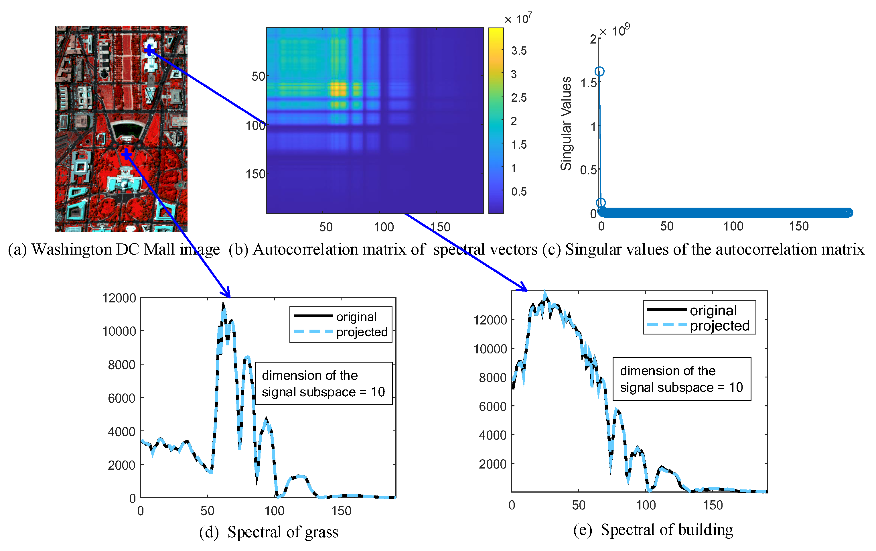
32], we generated noisy HSIs of Pavia University data (of size 310 (rows) × 250 (columns) × 87 (bands)), a subregion of Washington DC Mall data (of size 150 (rows) × 200 (columns) × 191 (bands)), and Terrain data (of size 500 (rows) × 307 (columns) × 166 (bands)).
For the first two datasets, we removed bands that were severely corrupted by water vapor in the atmosphere. To obtain relatively clean images, we projected spectral vectors of each image onto a subspace spanned by eight principal eigenvectors of each image. The projection of each image was considered to be a clean image. To simulate noisy HSIs, we added four kinds of additive noise into images as follows:
Case 1 (Gaussian non-i.i.d. noise): Synthetic data with Gaussian noise. The noise in ith pixel vector , where is a diagonal matrix with diagonal elements sampled from a uniform distribution .
Case 2 (Gaussian noise + stripes): Synthetic data with Gaussian noise (described in case 1) and oblique stripe noise randomly affecting 30% of the bands and, for each band, about 10% of the pixels, at random.
Case 3 (Gaussian noise + “Salt and Pepper” noise): Synthetic data with Gaussian noise (described in case 1) and “Salt and Pepper” noise with a noise density of 0.5%, meaning approximately 0.5% of elements in are affected.
Case 4 (Gaussian noise + stripes + “Salt and Pepper” noise): Synthetic data with Gaussian noise (described in case 1), random oblique stripes (described in case 2) and “Salt and Pepper” noise (described in case 3).
To evaluate the impact of denoising methods on the hyperspectral unmixing task, we simulated a clean semi-real HSI based on the publically available Terrain image (
Figure 4c) following generation steps in [
36]. A MATLAB demo used to generate a semi-real HSI is available at
https://github.com/LinaZhuang/NMF-QMV_demo, accessed on 8 October 2021. The original Terrain image has a size of 500 (rows) × 307 (columns) × 166 (bands) and is mainly composed of soil, tree, grass, and shadow. The number of endmembers is empirically set to 5, as performed in [
36,
46,
47]. Briefly, a clean Terrain image was synthesized based on a linear mixing model [
1]; i.e.,
, where
and
are endmembers and abundances, respectively, estimated from the original Terrain image. Next, we generated a noisy Terrain HSI by adding the Gaussian noise and oblique stripe noise (as described in case 2)—i.e.,
—yielding an MPSNR of 28.90 dB.
4.1.2. Comparisons
To thoroughly evaluate the performance of the proposed method, six state-of-the-art HSI denoising methods were selected for comparison: the fast hyperspectral denoising method (FastHyDe) [
8], the noise-adjusted iterative low-rank matrix approximation method (NAIRLMA) [
48], the spatio-spectral total variation based method (SSTV) [
49], the low-rank matrix recovery method (LRMR) [
15], double-factor-regularized low-rank tensor factorization (LRTF-DFR) [
21], and the
-norm based hyperspectral mixed noise denoising method (L1HyMixDe) [
32]. These compared methods were carefully selected. The FastHyDe served as a benchmark to see whether mixed noise could be simply addressed by Gaussian denoisers. The NAIRLMA, SSTV, and LRMR are from highly cited papers working on hyperspectral mixed noise based on low-rank and sparse representations. The LRTF-DFR and L1HyMixDe methods are subspace representation methods and remove noise by filtering the subspace coefficients of HSIs. All experiments were implemented in MATLAB (R2016a) on Windows 10 with an Intel Core i7-7700HQ 2.8-GHz processor and 24 GB RAM. A MATLAB demo of this work will be available at
https://github.com/LinaZhuang, (accessed on 8 October 2021) for the sake of reproducibility.
The size of the sliding window in the Hampel filter,
q, was fixed to 7. The dimension of the subspace,
p, for FastHyDe, LRTF-DFR, L1HyMixDe, and HySuDeep methods was estimated by HySime [
37] automatically. The other parameters of FastHyDe, NAILRMA, LRTF-DFR, and L1HyMixDe were set as suggested in their original references. We fine-tuned the parameters
and
in SSTV and parameters
r and
s in LRMR to obtain the optimal results.
For quantitative assessment, the peak signal-to-noise ratio (PSNR) index, the structural similarity (SSIM) index, and the feature similarity (FSIM) index of each band were calculated. The mean PSNR (MPSNR), mean SSIM (MSSIM), and mean FSIM (MFSIM) of the proposed and compared methods on Pavia University Data and Washington DC Mall Data are presented in
Table 2, where we have highlighted the best results in bold.
4.2. Mixed Noise Removal
We compare the proposed method HySuDeep with FastHyDe [
8], NAILRMA [
48], SSTV [
49], LRMR [
15], LRTF-DFR [
21], and L1HyMixDe [
32] methods in terms of MPSNR, MSSIM, and MFSIM (provided in
Table 2 and
Table 3). The band-wise PSNR is depicted in
Figure 5 for quantitative assessment.
Among the compared methods, only FastHyDe is shown to address pure Gaussian noise, not mixed noise. We include FastHyDe to evaluate whether mixed noise can be reduced by a simple Gaussian denoiser. As shown in
Table 2, FastHyDe outperformed other methods in case 1 (where HSIs are corrupted by only Gaussian noise). However, when the images were contaminated by mixed noise in Cases 2–4, the results of FastHyDe show that heavy mixed noise cannot be reduced well by a Gaussian denoiser. The existence of mixed noise in HSIs calls for effective denoising techniques.
To address mixed noise, an additive term is usually introduced to model sparse noise so that the entries in the data fidelity term, , follow Gaussian distributions. The proposed HySuDeep, NAIRLMA, SSTV, LRMR, and LRTF-DFR methods fall in this line of research. The critical differences among these methods are the regularizations imposed on the HSI, . SSTV minimizes the total variation of the HSI in the spectral–spatial domain. NAILRMR and LRMR impose spectral low-rankness in spatial patches of the image. LRTF-DFR and the proposed HySuDeep both enforce the low-rankness of spectral vectors by subspace representation. To exploit the spatial correlation of eigenimages, LRTF-DFR minimizes the spatial difference (i.e., total variation) of eigenimages, while HySuDeep uses a CNN-regularization (i.e., a deep image prior extracted from a CNN network).
The proposed method uniformly yields the best results in Cases 2–4, as shown in
Table 2 and
Table 3. The main reason is that, compared with SSTV, NAILRMR, LRMR, LRTF-DFR, and L1HyMixDe methods, our method uses a more efficient spatial regularization term. Although the CNN regularization works like a black box, we can see its superiority over TV regularization (used in SSTV and LRTF-DFR) and patch-based regularization (used in NAILRMA, LRMR, and L1HyMixDe) from
Table 2 and
Table 3. Furthermore, HySuDeep is similar to the L1HyMixDe method in terms of using subspace representations of spectral vectors and imposing a regularization on representation coefficients.
Table 2 and
Table 3 show that HySuDeep achieves better results than L1HyMixDe. The difference is caused by the accuracy of spectral subspace learning. Compared with L1HyMixDe, HySuDeep elaborates an outlier removal operator, which improves the estimates of subspace
(see discussion in
Section 4.3).
For visual comparison, we display the 37th band of Pavia University data and the 126th band of Washington DC Mall data in
Figure 6 and
Figure 7, respectively. For case 1 (Gaussian noise), all methods can reduce noise significantly. As shown in
Figure 6 and
Figure 7, SSTV and LRMR are able to remove light stripes, but still leave some wide stripes. Heavy noise still remains in the results of NAILRMA and FastHyDe. LRTF-DFR, L1HyMixDe, and HySuDeep methods visually yield comparable results in
Figure 6 and
Figure 7. To show their differences, we generated and presented the residual images in
Figure 8a,b, where we can see the results of proposed HySuDeep contain less residual compared with LRTF-DFR and L1HyMixDe.
4.3. Subspace Learning against Mixed Noise
One of the contributions of this paper is the introduction of an orthogonal subspace identification method that is robust to mixed noise. We conducted experiments using simulated images to compare the proposed subspace learning method with representative subspace learning methods: namely, SVD, RPCA, L1HyMixDe [
32], and HySime [
37]. Results are reported in
Table 4, where we show two metrics, namely
and
, measuring the relative power of the clean spectral vectors and noise lying in the estimated subspace, respectively.
In Case 1, two images were corrupted only by Gaussian noise, and values of for all methods are higher than 0.9993, implying that all the methods can estimate a subspace representing image signal very well. Case 3 shows results similar to Case 1; that is, all the methods achieve relatively high . We conclude that when noise is Gaussian distributed or a mixture of Gaussian and “Salt and Pepper” noise, signal subspace learning is not a challenging task and we can simply use SVD. The reason is that Gaussian noise and “Salt and Pepper” noise are randomly and uniformly distributed in each channel; thus, the noise increases singular values in the direction of each eigenvector almost uniformly and does not change the order of the singular values of clean images. The signal subspace is approximately spanned by p singular vectors of the noisy image corresponding to the largest p singular values.
However, subspace learning from noisy images in Case 2 and Case 4 is challenging and we cannot simply use SVD because the stripe noise usually exist in specific channels, instead of being uniformly distributed in all channels. The stripe noise will significantly increase the variances of those channels affected by stripe noise. Due to the fact that SVD tends to learn a subspace representing information in channels with high variances, SVD is not suitable for Case 2 and Case 4. This inference is consistent with the results in
Table 4, where SVD obtains the worst results in terms of
and
in case 2 and case 4. If we only focus on the table rows highlighted with gray color, the proposed learning method performs better than others. Among the compared methods, RPCA learns a subspace representing low-rank signal and excluding sparse noise. However, stripe noise is also low-rank [
50], and RPCA cannot separate an image signal and stripes using only a low-rank regularization. HySime is conceived based on an assumption of Gaussian noise and is clearly not suitable for mixed noise. L1HyMixDe performs median filtering band by band, exploiting spatial correlation, whereas HySuDeep estimates a coarse image using Hampel filtering pixel by pixel, exploiting spectral correlation. As shown in gray rows of
Table 4, HySuDeep uniformly provides the best performances.
4.4. Analysis of Regularization Parameters
There are two regularization parameters—namely,
and
—in the objective function of the proposed HySuDeep method. Controlling the trade-off between Gaussian noise reduction and detail preservation, the parameter
is related to the standard deviation of Gaussian noise, which can be estimated via (
25).
The second parameter
controls the sparsity of estimation of sparse noise
. The setting of
should depend on the intensity of sparse noise.
Figure 9 depicts the denoising performance of HySuDeep in the Pavia University image and in the Washington DC Mall image as a function of the value of parameter
. When the value of
is set to {1, 3, 5, 7, 9}, denoising results are acceptable in both images. Therefore, we simply set
to 3 in all experiments in this paper.
4.5. Numerical Convergence of the HySuDeep
Since CNN-regularization is incorporated into (
10), the proposed HySuDeep cannot be considered as a convex optimization problem; thus, its theoretical convergence is not guaranteed. However, its numerical convergence is systematically observed when the augmented Lagrangian parameters are set to
. As shown in
Figure 10, the relative change converges to near zero after 15 iterations, implying the convergence of the proposed method can be numerically guaranteed.
4.6. Application in Hyperspectral Unmixing
Hyperspectral denoising is usually implemented as a preprocessing step for subsequent applications. This subsection takes hyperspectral unmixing as an example to evaluate whether the image denoising step has a positive impact on the performance of subsequent applications. Spectral unmixing mainly involves two stages: (i) identifying materials present in the scene (termed endmembers) and (ii) estimating the fraction (or abundance) of each material in each pixel. The hyperspectral unmixing task was chosen considering that the endmember extraction step can be very sensitive to sparse noise.
We first performed denoising on the Terrain image using FastHyDe, NAILRMA, SSTV, LRMR, LRTF-DFR, L1HyMixDe, and HySuDeep. The mean PSNR (MPSNR), mean SSIM (MSSIM), and mean FSIM (MFSIM) of the proposed and compared methods on Terrain image are presented in
Table 3, where we have highlighted the best results in bold. Then, we unmixed the spectra of the denoised images by using vertex component analysis (VCA) [
53] to estimate the endmembers and used fully constrained least squares (FCLS) [
54] to estimate the abundances. Two metrics were computed: the normalized mean square error (NMSE) of endmembers
and abundances
, denoted as
and
, respectively. As reported in
Table 3, LRMR, LRTF-DFR, L1HyMixDe, and HySuDeep obtain a lower NMSE of endmembers than the counterpart image without denoising processing. For images denoised by FastHyDe, NAILRMA, and SSTV, the errors in the estimates of endmembers directly result in high errors in the estimates of abundances. Among LRMR, LRTF-DFR, L1HyMixDe, and HySuDeep, the proposed HySuDeep leads to the lowest NMSE of abundances.


