Assessment of the Temperature Effects in SMAP Satellite Soil Moisture Products in Oklahoma

Abstract

Soil moisture is a notably important component in various studies in water sciences, including hydrology, agriculture, and water management. To achieve extensive or global spatial coverage, satellites focusing on soil moisture observation have been launched, and many satellite products, such as SMAP and SMOS soil moisture products, have been provided. Most of these satellite observations are based on the dielectric properties of wet soil, and most soil moisture retrieval algorithms are calibrated or evaluated using in situ soil moisture. While the in situ data observed by dielectric sensors, which are the most widely used, are reported to include errors caused by the so-called “temperature effects” of these sensors, the temperature dependency of bulk soil dielectric constant has rarely been discussed on satellite data. Since both in situ dielectric measurements and satellite observations are based on the same physical variable, the dielectric constant and the dielectrically measured in situ soil moisture data are also used as ground truth, it is necessary to assess the impact of temperature effects on satellite products. In this work, we attempted to identify the existence of the temperature effects and evaluate the consequences of removing these effects on in situ and satellite soil moisture and the relationships between the brightness temperature at the soil surface and the brightness temperature provided by satellite observation. To achieve the goals of this study, we analyzed the temperature effects on surface soil moisture data provided by a SMAP mission in Oklahoma, the United States. The results show that temperature effects exist in SMAP soil moisture products in Oklahoma, and the removal of these effects will potentially improve the accuracy of these products.

1. Introduction

Soil moisture is widely known as one of the key factors controlling the processes of the hydrologic cycle, global energy, and water circulation [1,2]. The strategies relevant to water management, agricultural production, disaster forecast, and adaptation to climate change need precise and reliable soil moisture data, as these data are critical to conducting research. Thus, some techniques have been developed to obtain soil moisture data precisely. Conventionally, there are several methods to collect soil moisture estimation, such as in situ measurements, satellite remote sensing, and hydrological models. Moreover, other measured techniques have been employed recently, such as the cosmic-ray neutron probe or the global positioning system (GPS), to provide more chances for relevant studies [3,4]. However, each of these suffers from some limitations [5,6,7,8,9]. Although in situ data are known to provide the most reliable point-scale soil moisture estimation, they face a considerable restriction on regional coverage. Hence, large-scale spatial distribution of data is not yet available [10,11,12].

The number of extreme climate events has increased recently. It is necessary to establish techniques for collecting accurate soil moisture data globally to satisfy demands. Jackson and Schmugge [13] have proposed a new method to obtain surface soil moisture through remote sensing to overcome the limitation of in situ methods. Nowadays, many space missions with active and/or passive microwave sensors are being conducted to complement the drawbacks of ground-based observations [14,15,16,17]. Although many space projects have been retrieving soil moisture products from microwave radiometers since the 1970s, the first mission dedicated to soil moisture was Soil Moisture and Ocean Salinity (SMOS) that was launched in 2009. This instrument operates in the L-band (1.4 GHz), the optimal wavelength for soil moisture retrieval [18]. In 2015, the Soil Moisture Active Passive (SMAP) mission, which operates at the same frequency as SMOS, was launched to improve the accuracy, resolution, and global coverage of satellite soil moisture data by incorporating both an L-band radiometer (passive) and L-band radar (active) [19,20].

Nevertheless, the satellite-based datasets suffer from other obstacles relating to accuracy. Although many efforts have been made to improve the quality of satellite soil moisture estimation, the accuracy over some areas remains unsatisfactory [21]. These handicaps might be due to both the retrieval algorithms [22,23] and the reference source for the evaluation processes [24].

While in situ data have been used to calibrate the algorithm parameters and validate the satellite soil moisture data in many studies [23,25,26,27], several lines of evidence indicate that these datasets, especially dielectrically measured ones, contain errors relating to temperature fluctuation, known as temperature effects [28,29,30,31,32]. They are widely observed in dielectrically measured volumetric soil water content (hereafter referred to as “SWC”). The experiments of Wraith and Or [28] showed that the bulk soil dielectric constant (or permittivity ${\epsilon }_b$), which is used for deriving soil water content, depends on the soil temperature. Their experiments indicate that the ${\mathsf{\epsilon }}_{\mathrm{b}}$ sensor reading changes with temperature while the actual value of soil water content is kept unchanged. Schanz et al. [33] have verified these effects on soil water content with time domain reflectometry (TDR) measurement with experiments at different temperatures in a range between $20 °\mathrm{C}$ and $80 °\mathrm{C}$. Kapilaratne and Lu [29] confirmed that fluctuations in soil water content, synchronized with those of soil temperature, exist and are mainly caused by temperature effects. From their study, though the evaporation also causes diurnal variability, it differs from the soil moisture fluctuation in time series. While the diurnal variability from evaporation causes a low value of soil water content in the daytime and high value in the nighttime, the in situ soil moisture shows the inverse. In addition, many studies pointed out that temperature effects are one of the critical factors causing this diurnal variability. Lu et al. [30] proposed a data-driven method for successful removing temperature effects.

The satellite soil moisture products (SMAP and SMOS) are inferred from the brightness temperatures, the product of the emissivity, and the effective surface temperature. While several studies have discussed the significance of the effective surface temperature for the soil moisture retrieval process [34,35], the emissivity depending on bulk soil dielectric constant has not been extensively evaluated. Thus, the authors think that the temperature dependency of bulk soil dielectric constant will affect the emissivity and the inferred soil moisture such as SMAP soil moisture (SMAP SM). Though SMAP tried to avoid the impact of the difference in soil temperature at ascending and descending nodes by designing an orbit to make them 6:00 pm and 6:00 am [26], respectively, evaluations of the temperature difference between ascending and descending nodes and its impact on retrieved soil moisture is not enough. Therefore, the existence and influence of temperature effects on SMAP SM still need to be checked.

Moreover, the errors due to temperature effects in in situ data may cause the deflection of other processes, such as land surface and climate models or soil moisture retrieval, and the inaccurate ground truth may lead to improper calibration and validation. Though the ground truth data obtained by other methods not requiring dielectric constant can theoretically be used, many non-dielectric measurements cannot provide continuous observations and they are expensive. These largely limit data availability and will probably make the data analysis very difficult. Since SMAP products used in situ soil moisture as the core validation sites (CVSs) for the calibration and validation process [21,27], if the CVSs contain errors caused by temperature effects, they will propagate back through the calibration process and result in inappropriate geophysical parameter retrieval. The SMAP soil water content (hereafter referred to as “SMAP SWC”) is therefore also potentially affected by temperature effects. Thus, these effects may limit the quality of soil moisture observation from space.

Previous studies about the validation of satellite soil moisture products found that the soil temperature variability during the daytime is much larger than that during the nighttime, because the daytime radiations largely affect the daytime soil temperature. A similar phenomenon is also observed in soil moisture. Many researchers (such as Kaihotsu et al. [36]) tried to avoid this problem using data during nighttime. However, we think this high variability comes from the high variability of soil temperature and can be removed using our temperature effects removal algorithm. It is expected that the removal of temperature effects will make daytime data similar to nighttime data and make satellite soil moisture products better calibrated and validated.

Therefore, the objectives of this work are (1) to identify the existence of the temperature effects and (2) to evaluate the impacts of the removal of these effects on in situ and satellite soil moisture and the relationships between the brightness temperature at the soil surface and the brightness temperature provided by satellite observation.

2. Study Area and Data Description

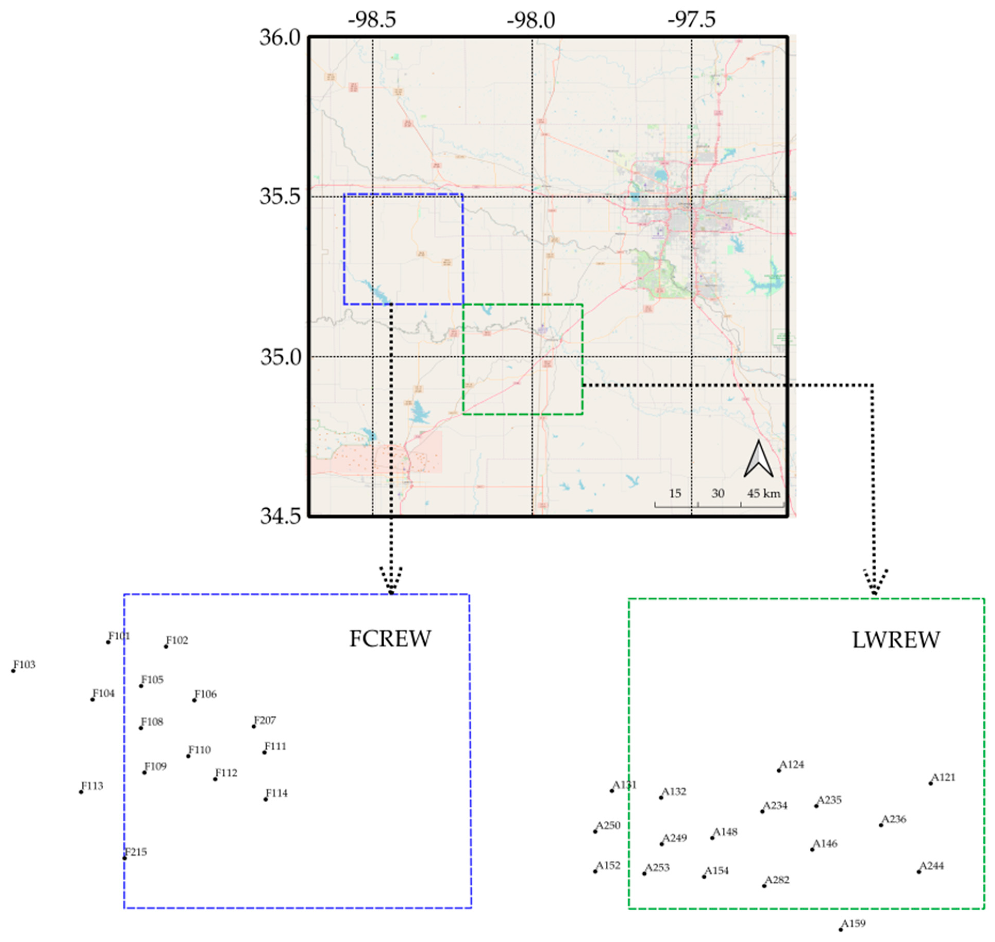
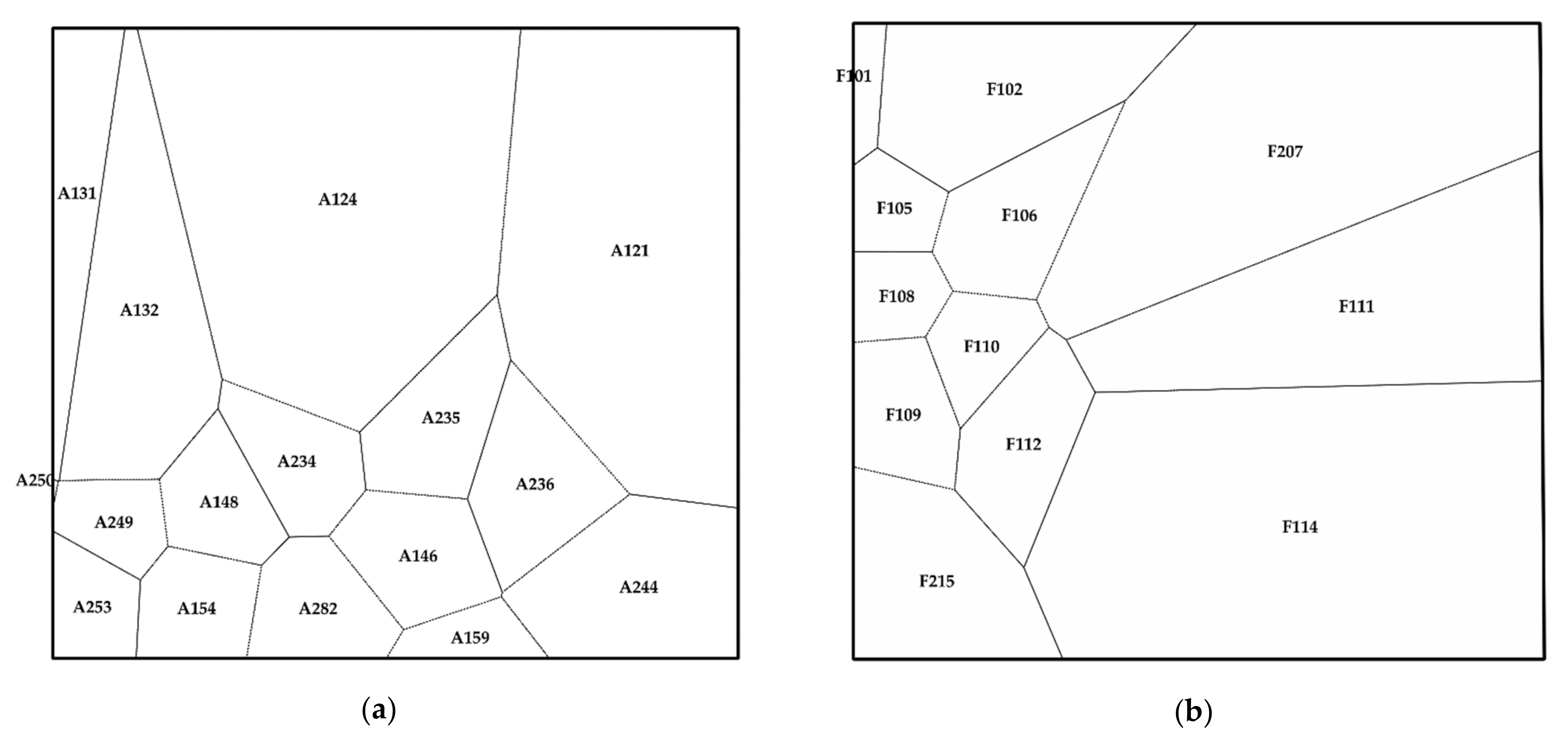
2.1. Study Area

Based on the conditions of the temperature effects removal method [30,37] and the accessibility of data widely used in the calibration and validation of SMAP soil moisture [21,27], we selected two sites of soil moisture for use in this study: the Little Washita River Experimental Watershed (LWREW) and the Fort Cobb Reservoir Experimental Watershed (FCREW), located in Oklahoma, the United States. The geographical description of these sites as well as the detail of station positions are shown in Figure 1. The LWREW site is popularly used to calibrate and validate many satellite soil moisture products [21,23,25,27,38]. These sites were known as the core validation sites (CVSs) in SMAP calibration/validation and selected to match the satellite footprint scale. These two CVSs cover the temperate climatic (Cfa) area (as categorized in the Köppen–Geiger climate classification [39]). As Jackson et al. [23] and Cosh et al. [40,41] reported, the topography of these sites is rolling with an altitude between 300 m and 600 m. The average elevation difference is about 200 m with few hills or outcrops. The landcover is dominated by grassland and cropland (mostly winter wheat). The soil textures range from silty loam to fine sand. The time zone of data used in this study is unified at local time. The detail of these CVSs is shown in

Table 1. The monitoring networks used in this study. Climates are classified following Peel et al. [39], where: C: temperate; f: without dry season; a: hot summer.

CVS Name	Elevation (m)	Pixel (Y/X)	Climate Classification	Annual Rainfall (mm)	Landcover
LWREW [23,40]	300–500	86/219	Cfa	760	Grassland
FCREW [41]	383–565	85/218	Cfa	816	Grassland/cropland

.

The distribution of the LWREW and FCREW sites represents pixels (86, 219) and (85, 218) of SMAP level 3 soil moisture (radiometer) products which employ the EASE-Grid 2.0 [42] (EASE2 grid) to specify the location of data pixels. Figure 1 describes the location of these pixels corresponding to the CVSs sites.

2.2. Data Description

2.2.1. In Situ Data

The examining sites were chosen based on some critical criteria, which are listed below. These criteria were selected depending on key aspects of the validation dataset mentioned in relevant studies such as Colliander et al. [27] or Lu and Kapilaratne [30].

• We make a comparison between the in situ and satellite data in this study. Therefore, these selected sites have to meet the conditions of the core validation sites for the SMAP level 3 soil moisture (radiometer) products (L3_SM_P), that Colliander et al. mentioned in their study [27] to adequately represent the footprint of satellite data;
• Some in situ networks restrict user access, or a public link is not available; these issues may be a limitation for further studies which would like to replicate this study. Hence, we suggest that the accessibility of in situ networks is one of the critical criteria;
• The availability of long, continuous dielectrically measured SWC along with temperature data at the same depth near the ground surface [30] is important for a better reflection of site condition. As referred from Kapilaratne and Lu’s [37] research, the duration of data has to be at least two years for analyzing the temperature correction coefficient, which will be discussed in the next section;
• The inserted probe direction at the sites has to be horizontal to avoid the potential effect of vertical gradients of SWC and soil temperature [37] and the vertical heterogeneity of soil temperature variation, as mentioned in recent studies [43,44].

Regrettably, there are only a few sites that entirely satisfy these criteria in the world. To our knowledge, only the Agricultural Research Service’s Micronetwork (ARS) [41] matched these conditions. These databases are easily accessible via the website of USDA ARS’s Micronetwork (http://ars.mesonet.org/, accessed on 11 October 2021). For this study, we accessed the website and downloaded the data from 8 December 2020 to 4 February 2021.

The sensors of the Micronetwork stations are Steven’s HydraProbes installed horizontally in the soil at depths of 5, 25, and 45 centimeters below the ground surface [41]. The soil water content sensors are comprised of soil temperature sensors. This study uses the soil water content and soil temperature at a 5-centimeter depth corresponding to the satellite soil moisture observation. Additionally, we also used precipitation data to investigate the influence of temperature on both SWC and SMAP SWC and remove its effects. The ARS website provides both 5-minute and 24-hour temporal resolution for SWC, soil temperature, and rainfall data. In this study, we reformatted the 5-minute data to an hourly interval for conducting the analysis.

While doing the first assessment to conduct this study, we found that the soil moisture dataset at some stations contained errors, such as breaks, valleys, or spikes, as mentioned by Dorigo et al. [45]. These erroneous data were excluded before conducting the analysis.

Since the CVSs represent soil moisture distribution within the pixels, a weighted average method was applied to calculate the average values for the CVSs. According to Colliander et al. [27], the CVSs presenting 36 km pixels should have at least eight stations to ensure the confidence level is 70% for 0.03 m³/m³ soil moisture uncertainty with 0.07 m³/m³ variability [27]. Hereafter, the “in situ data” term is referred to as the weighted average data. The following part and

Table 2. Details of the in situ soil moisture data at the study sites.

CVS Name	The Sensors of Soil Moisture	Measurement Depth (cm)	Period	Number of Stations	Standard Deviation of the Average Values
LWREW	HydraProbe Digital Sdi-12 (2.5 volts)	5–5	September 2017–December 2019	16	0.0187
FCREW	HydraProbe Digital Sdi-12 (2.5 volts)	5–5	October 2016–December 2019	12	0.0186

describe the details of each CVS used in this study.

The Little Washita River Experimental Watershed

The LWREW core validation site belongs to the 610 km² watershed of Little Washita River that covers pixel (86, 219). In 1993, the ARS started monitoring the mesoscale environmental measurement system with a 43-station network in Oklahoma [46] to meet many needs in agriculture, water resource, and natural resource policy research. Forty-two of the 43 stations began operating from 1993 through 1994. One station (B123) was commissioned in 1997 (http://ars.mesonet.org/, accessed on 11 October 2021). However, the research objectives of the project have changed over time; some stations have been retired or relocated with other nearby stations. Currently, the LWREW comprises 20 stations of instrumenting. Because of its long historical record of data, the LWREW is widely used in long-term soil water studies.

Three of twenty stations were eliminated due to long-missing data (NaN values). Seventeen stations, as shown in Figure 1, have been selected for creating the Thiessen polygons. Only 16 of the 17 stations contribute within the pixel. The standard deviation of the average value is about 0.187 m³/m³. Moreover, the soil moisture uncertainty is 0.025 m³/m³ at the 80% confidence level. Figure 2a presents the Thiessen polygons at the LWREW used for weighing the in situ data.

Fort Cobb Reservoir Experimental Watershed

The FCREW core validation site covers pixel (85, 218), which the Fort Cobb Reservoir Experimental Watershed encloses. This watershed spreads over an area of 786 ${\mathrm{km}}^2$. The FCREW stations began instrumenting in 2005 as part of the Conservation Effects Assessment Project (CEAP) launched in 2003. For the CEAP study, some of the LWREW research instruments have been relocated to create the FCREW [47]. A total of 15 stations were redirected from the LWREW stations to address new research goals.

Though the data quality of all 15 stations is usable, because only 12 of the 15 stations contribute weight to pixel (85, 218), the in situ measurements were averaged from the Thiessen polygons of the FCREW, as shown in Figure 2b. The standard deviation of this average is about 0.186 m³/m³, along with the 0.025 m³/m³ soil moisture uncertainty (80% confidence level).

2.2.2. Satellite Data

The SMAP level 3 soil moisture (radiometer) products (hereafter referred to as “SMAP products”), which belong to the SMAP mission [17,20,26], were used to examine the temperature effects in satellite soil moisture data. In general, the L-band radiometer (1.41 GHz) collected brightness temperature (TB) data every two or three days to satisfy one of the SMAP mission’s objectives. According to the SMAP mission, which launched on 31 January 2015, the “tau-omega” model was used to compute the near-surface soil moisture at 5-centimeter depth using the SMAP radiometer Level-1C data at a spatial resolution of 36 km [13,22,26].

The SMAP data used in this study were obtained from the Application for Extracting and Exploring Analysis Ready Samples (AppEEARS) website (https://lpdaacsvc.cr.usgs.gov/appeears/, accessed on 11 October 2021), which belongs to the EarthData system, from 10 February 2021 to 18 March 2021. The ascending (hereafter referred to “ASC”) and descending (hereafter referred to “DES”) orbits of the SMAP products are 18:00 and 06:00 at the local time, respectively.

3. Methods and Results

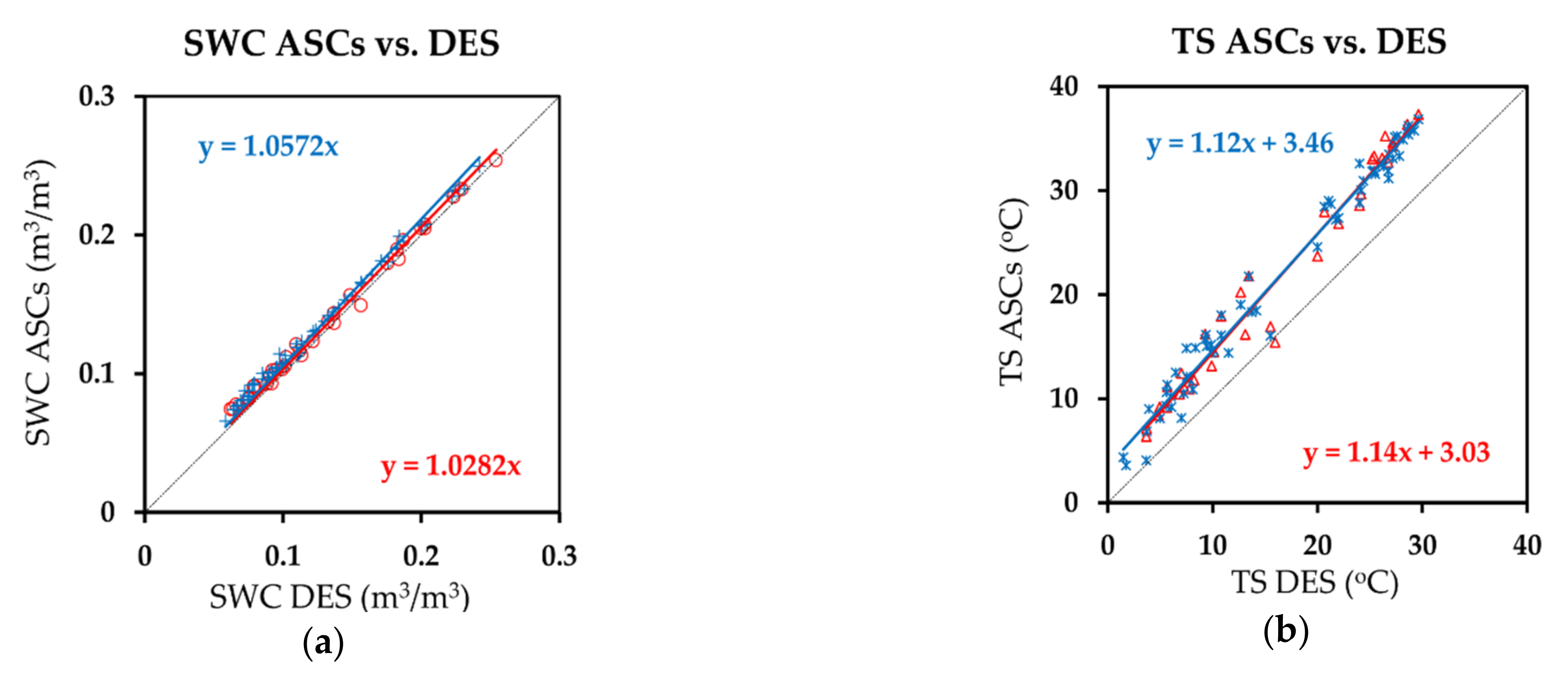
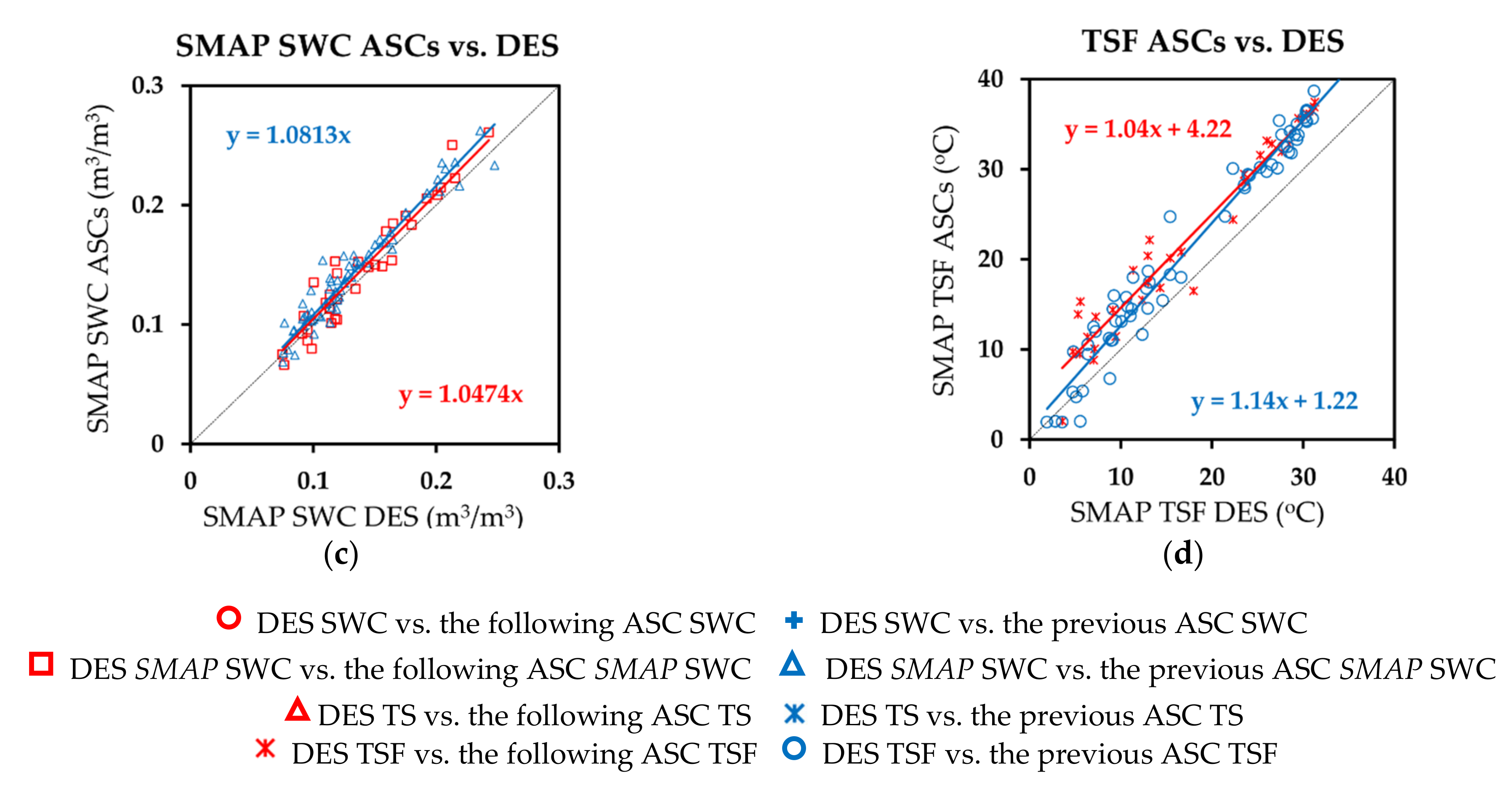
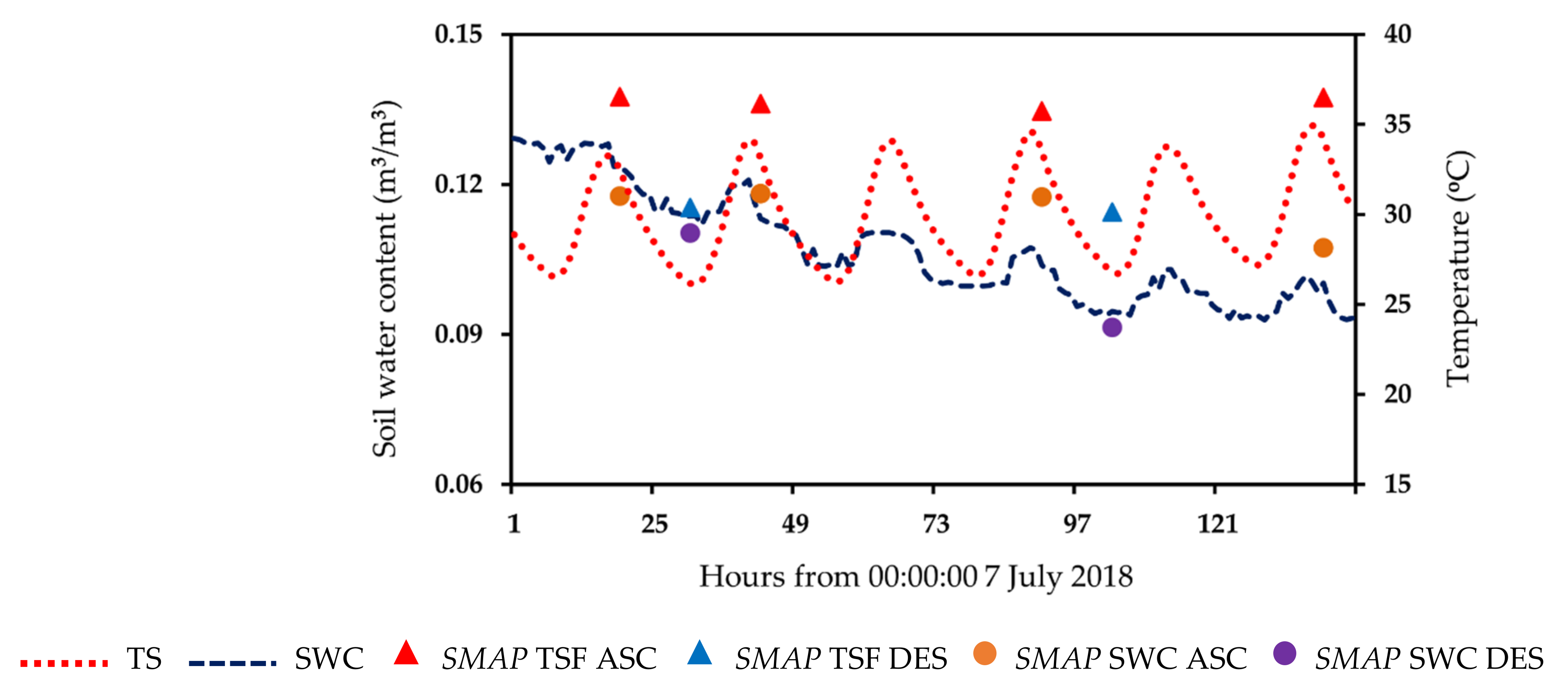
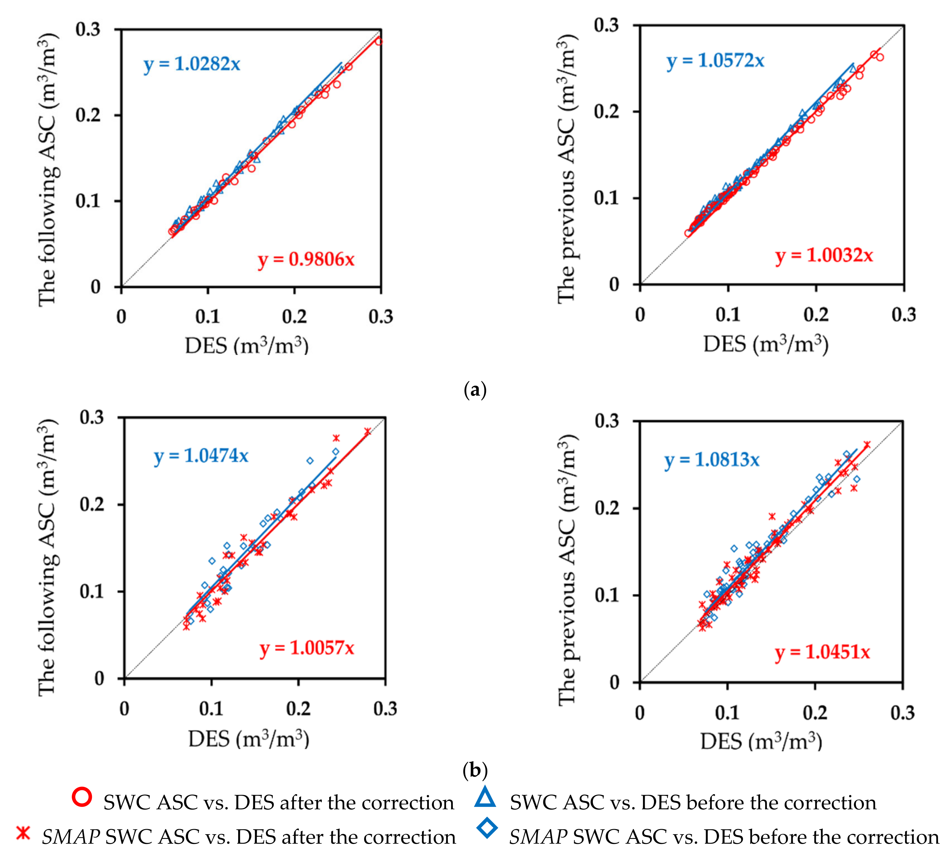
3.1. Analyzing the Trend of ASC and DES Soil Moisture from Both Retrieval Products and In Situ Observations

In order to determine the temperature effects on the SMAP SWC, we assessed the relationship between SMAP SWC and other factors, such as soil temperature or SMAP surface temperature (hereafter referred to as “SMAP TSF”). The assessment had two parallel steps. They include inspection of the relationship between both previous and following ASC and DES of both SMAP and in situ data to check the trend of the SMAP SWC.

The correlation analysis was carried out in both examinations to identify the relationship between ASC and DES temperatures and soil water content of both in situ and SMAP data, respectively. Since SMAP products do not provide the soil temperature, the retrieval surface temperature was used as a replacement to evaluate the relationship between soil water content and temperature factor in satellite data. To compare the satellite and in situ data equally, we extracted values at the ASC and DES nodes from the hourly in situ data for conducting the analysis. Only days comprised of both ASC and DES nodes of SMAP data were selected for these analyses.

Figure 3 presents the results of both the first and second investigations. In the first analysis, the red circles and triangles stand for the relationship between values at the descending and following ascending nodes of the SWC and TS at a 5-centimeter depth, respectively. The red squares and stars represent the correlation between values at the descending and following ascending nodes of the SMAP SWC and SMAP TSF, respectively. It clearly shows that the morning soil moistures (DES) tend to take lower values than the evening ones on the same day for both in situ and satellite data. In addition, the evening temperatures (from both in situ and SMAP) are significantly higher than the morning ones.

Turning to the second analysis, we examined the relationships between the DES and the previous ASC values of both in situ and satellite data. In Figure 3, the trend of SWC values plotted by blue pluses also follows the trend of soil temperature, which is represented by blue stars. In the satellite data, a similar phenomenon is seen as well. In this analysis, both retrieval and in situ morning soil moisture also show lower values than the previous evening ones. Taking the first and second analyses together, it indicates that the soil moisture goes up in the evening (ASC) and down back in the morning (DES). Moreover, this trend follows the direction of temperatures.

The two analyses demonstrate that the ASC values tend to be larger over three continuous values than the DES ones. However, the discrepancies between the previous ASC and the DES values are slightly higher than the same-day ones. Though the relationship between the previous ASC and the DES values can be explained by the reduction caused by evaporation and vertical redistribution of infiltrated water, the increase at the following ASC node is difficult to explain physically. Thus, it is reasonable to consider that this trend may be caused by the higher temperature at ASC nodes, an apparent increase named temperature effects.

A diagram of hourly in situ and SMAP data at ascending and descending nodes during six days was plotted together for a visual presentation to show the phenomenon more clearly. Figure 4 provides an overview of the trend in soil moisture and temperature. In Figure 4, the diurnal changes in SWC follow those in soil temperature, as mentioned in the Introduction. On the other hand, the SMAP SWC at ascending and descending nodes, which is plotted as orange and purple dots, tends to follow the fluctuation of the SWC; the SMAP TSF agrees with the soil temperature tendency as well. Furthermore, Figure 4 also shows that the morning retrieval soil moisture always takes lower values than the evening one; this trend associates with the direction of SMAP TSF.

To confirm, the following section will discuss the impacts of temperature effects removal on both in situ and satellite retrievals.

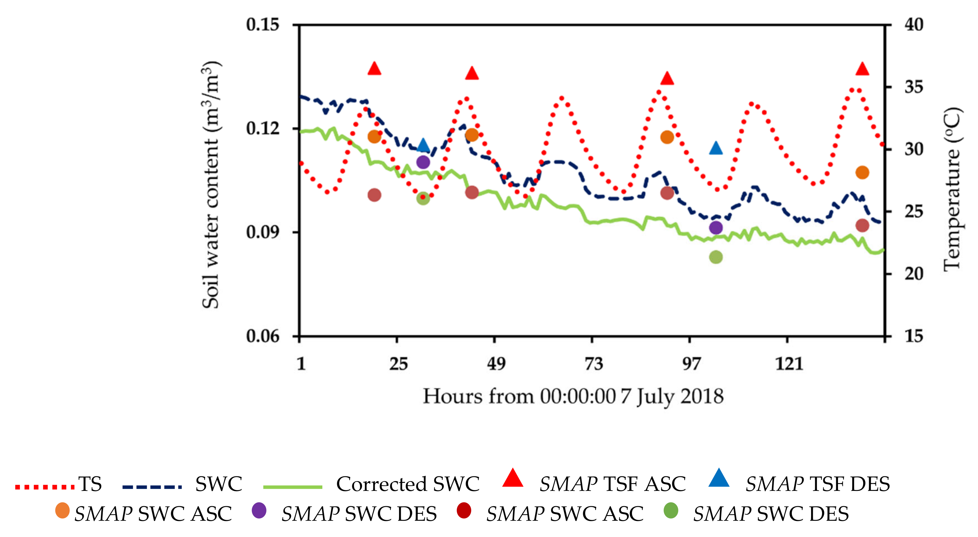
3.2. Temperature Effects Removal

The previous section indicated that the trend of soil moisture values corresponds to the temperature changes from both satellite and in situ data. While the SMAP SWC follows the SMAP TSF trend, the SWC agrees with the diurnal changes of TS. In order to confirm the contribution of temperature effects on the discrepancy between ascending and descending SMAP SWC values as well as on the diurnal changes of SWC, we applied the temperature effects removal method proposed by Lu et al. [30], to remove and evaluate their impacts. This method has been used to remove temperature effects from in situ soil water content data effectively. According to Lu et al. [30], Equation (1) can be used to express the temperature effects on the measured SWC by examining the correlation of the amplitude of the SWC against the amplitude of soil temperature and daily mean SWC:

$$A_{\theta }=\alpha {\theta }_d{A}_T$$

(1)

where $A_{\theta }$ and $A_T$ stand for the daily amplitudes of SWC and soil temperature, respectively; $\alpha$ represents a temperature correction coefficient; and ${\theta }_d$ is the daily mean SWC.

Before analyzing the relationships between $A_{\theta }$, $A_T$, and ${\theta }_d$ to determine the $\alpha$ value, the days with subsequent days having a daily rainfall amount greater than 0.1 mm, and days influenced by rainfall were excluded, in order to avoid an abrupt increase in the amplitude of the SWC due to rainfall [37]. Moreover, the days with a below-freezing soil temperature were also eliminated to prevent the influence of drastic changes in the bulk dielectric permittivity of the soil when the water is in a frozen state [31].

Kapilaratne and Lu [37] proposed Equation (2), an expansion of Equation (1) into a general form for expressing actual and measured SWC as a function of actual and reference temperature, to calculate the actual SWC:

$$\theta -{\theta }_{ref}=\alpha {\theta }_c\left(T-T_{ref}\right)$$

(2)

where $\theta$ and ${\theta }_{ref}$ represent the measured and reference SWC at $T$ and $T_{ref}$, respectively; $T$ is the actual soil temperature and $T_{ref}$ is a temperature at which the calibration curve was created; ${\theta }_c$ expresses the SWC at temperature $T_c$, which is between T and $T_{ref}$. The calibration curve is a tool to convert the SWC from the measured dielectric permittivity of the soil, usually available from the sensors.

From Equation (2), a correction formula is applied by approximating ${\theta }_c$ with ${\theta }_{ref}$. Lu et al. [30] also indicated that a change of $20 °\mathrm{C}$ in the soil temperature amplitude can cause a 16% relative error in the actual SWC ($T_{ref}=20 °\mathrm{C}$). From Equation (3), the ${\theta }_{ref}$ is known as the corrected SWC, which is taken as the actual SWC:

$${\theta }_{ref}=\frac{\theta }{1+\alpha \left(T-T_{ref}\right)}$$

(3)

Similarly, we used Equation (4), a derivation of Equation (3), for removing the temperature effects from the SMAP SWC. However, two points of data (ASC and DES) cannot be used to calculate the amplitudes because the exact minimum and maximum of the fluctuation cannot be captured. Thus, we used the temperature correction coefficient $\mathsf{\alpha }$ derived from in situ SWC in Equation (1) for computing. This issue is also a limitation for globally correcting the satellite data since the removal method depends on in situ data. Although some studies showed that the soil temperature corresponding to the satellite soil moisture is better [35], unfortunately it is not available in SMAP products. Therefore, in Equation (4), the soil temperature is replaced by the SMAP surface temperature since these two variables are closely related. Though the SMAP TSF had only two points of data at ascending and descending nodes and was not able to reflect the diurnal change in the soil moisture, these datapoints indicated a trend of temperature during the investigating period: higher values at dusk and lower values at dawn. For this reason, the authors chose SMAP TSF as a variable to replace soil temperature. The reference SMAP SWC ($SMA{P}_{ref}$) value in this Equation is known as “SMAP SWC data after correction” and is viewed as the actual SMAP SWC value without temperature effects:

$$SMA{P}_{ref}=\frac{SMAP}{1+\alpha \left(TSF-T_{ref}\right)}$$

(4)

where $SMAP$ is the recorded SMAP SWC at $TSF$; $TSF$ stands for the SMAP surface temperature.

To evaluate the influence of the temperature effects removal method on retrieval soil moisture, we use the standard statistical metrics to investigate the relationships between ascending and descending soil moisture, and between in situ and satellite data before and after the correction. Concurrently, we analyze the correlation between the emission from the soil before and after correction and the retrieval brightness temperature of all polarization, to assess the impacts of temperature on both soil moisture and brightness temperature. Therefore, we carried out three analyses to evaluate the temperature effects on the SMAP SWC. For each analysis, tests both before and after correction were conducted to appraise the results. Figure 5 shows a schematic of the removal and analyzing procedures.

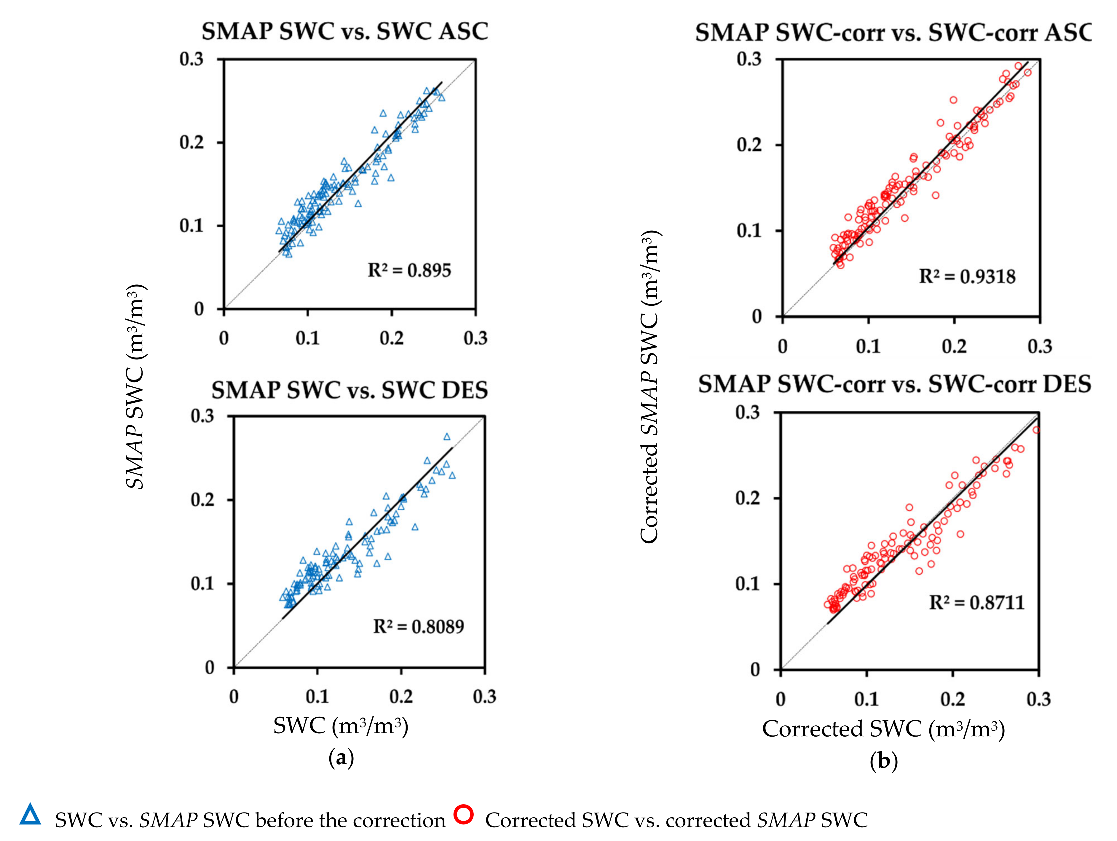
3.2.1. Examining the Temperature Dependency of SMAP Soil Moisture after Correction

This section discusses the tendency of the corrected SMAP SWC values at ascending and descending nodes after applying the temperature effects removal method.

First, the values of soil moisture ASC before and after correction were plotted against DES ones to evaluate the impact of temperature effects removal. Then, we checked the results of both the previous and following days of ascending soil moisture versus descending ones.

In Figure 6, the red symbols stand for the corrected data. It clearly shows a decrease of the discrepancy between ASC and DES soil moisture after removing the temperature effects from both in situ and satellite data. All the regressors of the correction are asymptotically close to unity. Figure 6b shows that the discrepancies between morning and the same day as well as the previous evening soil moisture retrieval have reduced after applying the temperature effects removal. Their regressors are closer to unity by about 4%. We can also observe a similar trend in the in situ data, which are presented in Figure 6a. These results demonstrate that the ascending values have become closer to the descending ones after correction. Both in situ and satellite results indicate that the previous ascending and descending discrepancies still remain substantial after the correction. This phenomenon can account for the evaporation and vertical redistribution of infiltrated water. All these outcomes imply the existence of temperature effects in SMAP SWC, and their removal can eliminate their effects.

Figure 7 presents the before and after correction, hourly in situ and SMAP data during six days, as an example. From this figure, the solid light green line stands for the corrected SWC, which shows that the diurnal SWC has most been removed by the temperature correction method. The corrected SWC tends to go down in the following day. Moreover, the discrepancy with the SMAP SWC decreases after removing the temperature effects. It can be observed that the corrected SMAP SWC at the ascending and descending nodes, illustrated by the wine-red and green dots, respectively, better follows the trend of the corrected SWC. Moreover, the morning retrieval soil moisture is closer to the evening ones. In other words, the discrepancy between both following and previous ascending and descending nodes of the corrected SMAP SWC is reduced after the temperature effects removal.

Additionally, the ASC SMAP SWC values tend to decrease more than the DES ones; the corrected SWC also exhibits a stronger reduction during daytime than nighttime. As we expected, the high variability of soil water content between daytime and nighttime, caused by the heterogeneity of soil temperature, disappears after applying the temperature effects removal. This result verifies the effects of temperature in the SMAP SWC.

3.2.2. Evaluating the Relationship between Satellite and In Situ Soil Water Content

To address another significant aspect of temperature effects removal, we analyzed the relationship between satellite products and in situ data, known as the ground truth for evaluating the performance of satellite products. Two standard statistical analyses were carried out in parallel to examine the correlation between two pairs of factors: SWC and SMAP SWC, and corrected SWC and corrected SMAP SWC. Figure 8 shows an improvement in the correlation between the satellite and in situ SWC at the LWREW site after applying the temperature effects removal method. Furthermore, it can be seen that the correlation between the corrected SWC and corrected SMAP SWC is stronger than between the SWC and SMAP SWC.

Table 3. The changes in the relationship between satellite and in situ data after applying the temperature effects removal method.

CVS Name	$\mathit{\alpha }$ (°C−1)	SWC vs. SMAP SWC (R2)		Corrected SWC vs. Corrected SMAP SWC (R2)		%Change
		ASC	DES	ASC	DES	ASC	DES
LWREW	0.0096	0.8950	0.8089	0.9318	0.8711	4.11	8.64
FCREW	0.0088	0.8016	0.7275	0.8571	0.8103	6.92	11.38

provides a summary of the correlation analysis for the relationship between satellite and in situ data.

Table 3 shows that, after removing the temperature effects, the R² at all sites increased significantly, especially at FCREW. Moreover, the significance values of the correlation between the satellite and in situ data are very small, and they have improved after removing the temperature effects. According to Lu et al. [30] and Kapilaratne et al. [29,37], the corrected SWC value is much closer to the actual SWC and can be viewed as the ground truth. Therefore, it can be said that the removal made the relationship between satellite soil moisture and in situ soil moisture better.

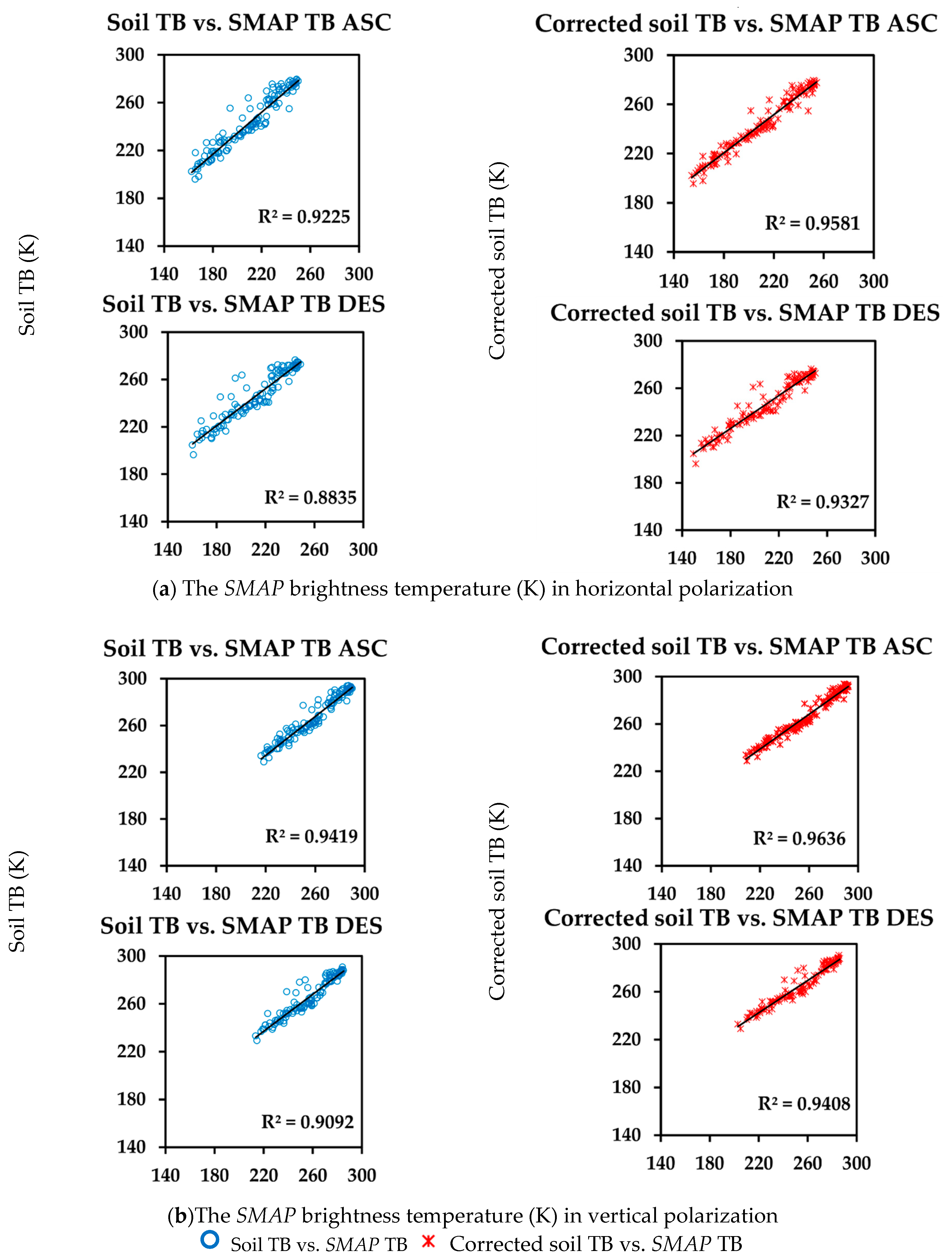
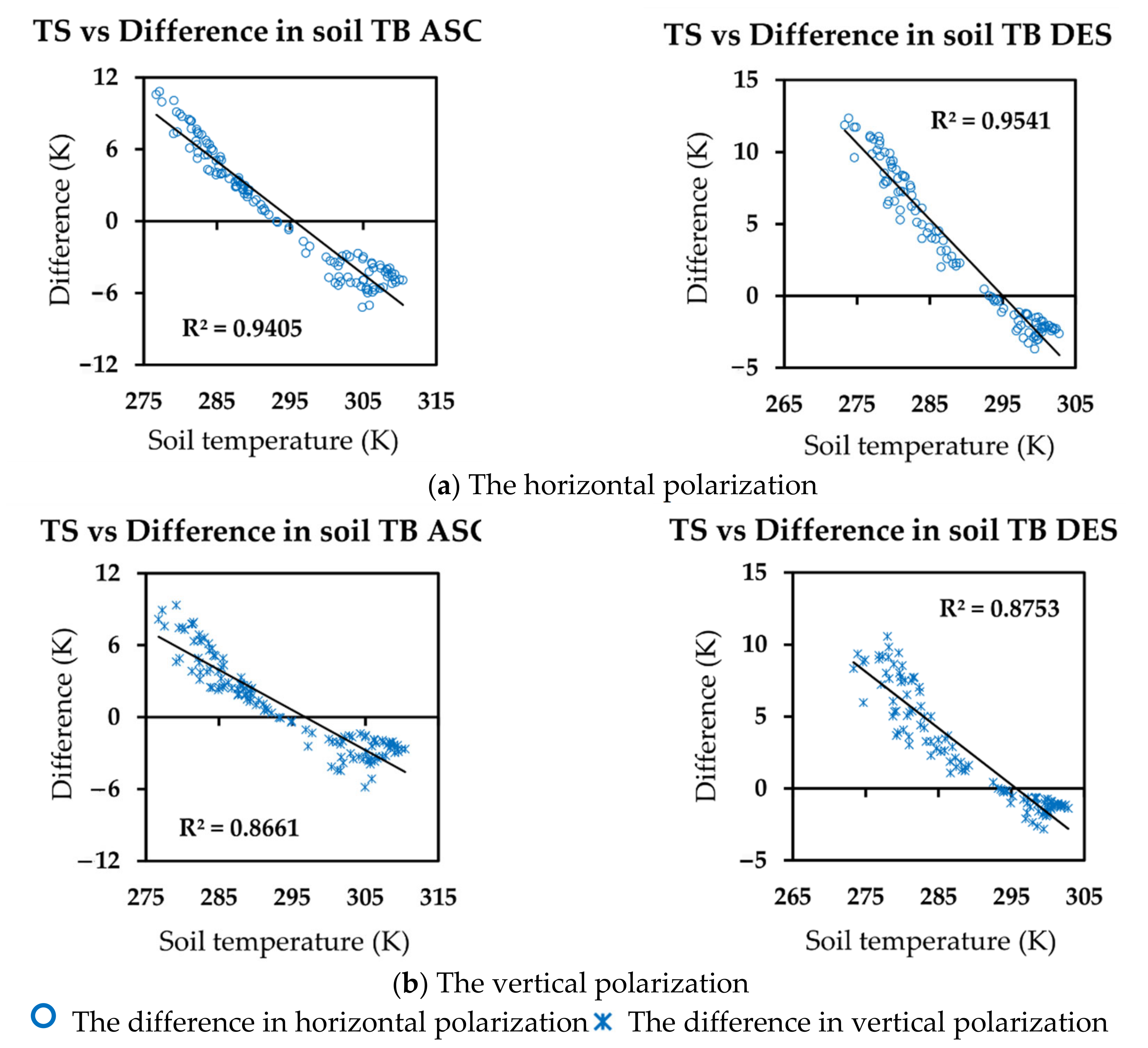
3.2.3. Evaluating the Impact of Temperature on Brightness Temperature at Soil Surface

The previous sections discussed the difference in trend between the morning and evening retrieval soil moisture and examined the impact of temperature effects removal on the discrepancy. Considering another way that the temperature effects can impact the retrieval process, we calculate the soil brightness temperature from the SWC and investigate the influence of temperature effects.

The Algorithm Theoretical Basic Document for SMAP products [26] shows that the radiative transfer equation includes soil and overlying vegetation canopy emissions. However, for the purposes of this study, we only focus on the contribution of the soil layer to the radiative transfer. Therefore, Equation (5) can be used to express the microwave brightness temperature:

$$T_{Bp}=e_p{T}_S$$

(5)

where the subscript p refers to the polarization (V—vertical or H—horizontal); T_B is the brightness temperature from soil (hereafter referred as to “soil TB”); e and T_S stand for the soil emissivity and the effective soil temperature, respectively.

To solve Equation (5), we need to determine two factors: the effective soil temperature and the soil emissivity. According to Wigneron et al. [35], the soil temperature can be referred to as the effective soil temperature since the emissivity is related to the reflectivity by $e_p=\left(1-r_p\right)$.

The soil reflectivity can be written as the Fresnel equation, which is shown below:

$$r_H\left(\phi \right)={\left|\frac{cos\phi -\sqrt{\epsilon -si{n}^2\phi }}{cos\phi +\sqrt{\epsilon -si{n}^2\phi }}\right|}^2\mathrm{and} r_V\left(\phi \right)={\left|\frac{\epsilon cos\phi -\sqrt{\epsilon -si{n}^2\phi }}{\epsilon cos\phi +\sqrt{\epsilon -si{n}^2\phi }}\right|}^2$$

(6)

where ${\mathrm{r}}_{\mathrm{H}}$ and ${\mathrm{r}}_{\mathrm{V}}$ represent the soil reflectivity in the horizontal and vertical polarization, respectively; $\phi$ is the SMAP incidence angle of $40°$; $\epsilon$ refers to the complex dielectric constant of the soil layer.

Finally, the complex dielectric constant in Equation (6) can be obtained by applying the generalized refractive mixing dielectric model [48,49], which is described in Equation (7):

$$\epsilon \prime =n^2-k^2 \mathrm{and} \epsilon ″=2nk$$

(7)

$$\epsilon \prime =n^2-k^2 \mathrm{and} \epsilon ″=2nk$$

(8)

$$k=\left\{\begin{array}{cc}{k}_d+k_b\theta ,& \theta \le {\theta }_t\\ k_d+k_b{\theta }_t+k_u\left(\theta -{\theta }_t\right),& \theta \ge {\theta }_t\end{array}\right.$$

(9)

where $\epsilon \prime$ and $\epsilon ″$ are the real and imaginary parts of the complex dielectric constant, respectively; $n$,$n_d$, $n_b$, and $n_u$, and $k$, $k_d$, $k_b$, and $k_u$ stand for the values of refractive index and normalized attenuation coefficient for moist soil, dry soil, bound soil water, and free soil water, respectively; $\theta$ and ${\theta }_t$ represent the SWC and the value of the maximum bound water fraction in a given type of soil, respectively.

The values of ${\theta }_t$, $n_d$, $n_b$, $n_u$, $k_d$, $k_b$, and $k_u$ can be obtained from the functions of clay content and temperature [49]. The clay content is the percentage of clay in the soil, which is provided from the SMAP dataset for each pixel covering the LWREW and FCREW sites. As discussed by Wigneron et al. [35], the soil temperature is used for these calculations. Through the complex dielectric constant calculated by the generalized refractive mixing model, the soil TB showed its dependency on soil temperature. For a SWC of 0.2 ${\mathrm{m}}^3/{\mathrm{m}}^3$ which is near the average in the study areas, the soil TB increases 10.7% while the soil temperature changes from 0 to $40$ °C. In this section, we attempt to calculate the soil TB from the SWC and corrected SWC, then investigate their relationship with the brightness temperature, which is available from SMAP products (hereafter referred to as “SMAP TB”), to examine the temperature effects on brightness temperature through the SWC. After applying the SWC and corrected SWC in (8) and (9), we get two values of the soil TB labelled as before and after correction. Figure 9 and

Table 4. The changes in the coefficients of determination of the regression between soil TB and SMAP TB of all polarizations at the ascending and descending nodes, at all sites.

Sites/Polarization		$\mathit{\alpha }$ (°C−1)	Ascending (R2)			Descending (R2)
			Before Correction	After Correction	%Change	Before Correction	After Correction	%Change
LWREW	H V	0.0096	0.9225 0.9419	0.9581 0.9636	3.86 2.30	0.8835 0.9092	0.9327 0.9408	5.57 3.48
FCREW	H V	0.0088	0.8796 0.9161	0.8994 0.9320	2.25 1.74	0.8531 0.9033	0.8866 0.9252	3.93 2.42

are used for presenting the results of these analyses.

Although two independent sources were used for deriving the brightness temperature to ensure an objective comparison, the values of these brightness temperature sources should be close together. As expected, Figure 10 shows a better correlation between the soil TB calculated from the corrected SWC and the SMAP TB at all polarizations for both ascending and descending nodes at the LWREW. A similar trend is also observed at the FCREW site. The details of the changes at all investigated sites are summarized in Table 4.

To quantify the impacts of temperature effects on soil TB, we conducted an analysis of the temperature and the magnitude of changes of soil TB. The differences in soil TB were computed as “Difference = Soil TB before correction—Soil TB after the correction”. The results are shown in Figure 10 for the LWREW site. To have a fair comparison, we changed the unit of soil temperature from degree Celsius to Kelvin.

Figure 10 illustrates clearly that the soil temperature significantly impacts the soil TB, especially in the evening time (ASC). Moreover, these differences relate to the variations of soil temperature.

Table 5. The variations of soil TB at all polarizations at both ascending and descending nodes at all sites.

Sites/Polarization		$\mathit{\alpha }$ (°C−1)	Absolute Changes in ASC (K)		Absolute Changes in DES (K)
			Minimum Change	Maximum Change	Minimum Change	Maximum Change
LWREW	H V	0.0096	0.03 0.02	10.79 9.33	0.01 0.01	12.32 10.56
FCREW	H V	0.0088	0.00 0.00	10.76 9.56	0.05 0.04	11.2 9.3

summarizes the variations of soil TB (the differences of soil TB before and after correction) resulting from the SWC and the corrected SWC. A similar trend in the differences between before and after temperature effects removal was also observed at the FCREW in Table 5. The overall trend shows the dependency of the soil TB on the soil temperature. The ranges of difference at ascending nodes tend to be larger than at descending ones. This trend follows the results of previous sections: the ascending retrieval soil moisture takes higher values than the descending ones and experience a larger reduction after the correction.

4. Discussion

This study confirmed the existence of temperature effects on SMAP SWC by analyzing the relationship between temperature and SMAP SWC in two research directions. First, we assessed the behavior of ascending and descending SMAP SWC corresponding to the soil temperature fluctuations and SMAP surface temperature trend. Second, we applied the temperature effect removal algorithm to both SMAP SWC and SWC to affirm the contribution of temperature effects. All analysis results show that the trend of SMAP surface temperature and SMAP SWC at ascending and descending nodes is in agreement with the fluctuations in in situ soil temperature and SWC. These findings imply that the temperature effects may cause a discrepancy between ascending and descending SMAP SWC, which needs to be removed to improve the quality of satellite soil moisture data.

In the second direction of research, the temperature effects removal method was used to correct both SWC and SMAP SWC data. The results indicate that the quality of the SMAP SWC data improved after removing the temperature effects, since the discrepancy between ASC and DES SMAP SWC became smaller than before the removal. Additionally, the regressor of ascending and descending SMAP SWC is asymptotically closer to unity by 3% to 4% than before the correction. Finally, it demonstrates that the ASC and DES SMAP SWC values were closer after the correction, and the trend of the morning soil moisture (DES) having lower values than the evening ones was eliminated after applying the temperature effects removal method.

Furthermore, the analyses on the correlation between satellite and in situ SWC both before and after removing temperature effects indicated that the corrected SMAP SWC and the corrected SWC had a better correlation than the SMAP SWC and the SWC at both the ascending and descending nodes at all selected sites. The averaged determination coefficient of the regressions between the corrected SMAP SWC and the corrected SWC increased by about 7.8% after removing the temperature effects, and the minimum improvement was 4.1%. The most impressive result was obtained for the FCREW site, where the relationship between satellite and in situ data went from a fair (0.7275) to a good correlation of about 0.8103 after the correction. This change is also a significant improvement, with an 11.38% increase in the determination coefficient of the regressions. This result suggests that the correction enhanced the relationship between satellite and in situ SWC at all selected sites and indicates that the corrected SMAP SWC values are in better agreement with the corrected SWC values.

Finally, we analyzed the relationship between the brightness temperature from the soil, which is the source variable for the retrieval of soil moisture, and SMAP brightness temperatures at all polarizations. These two values were considered as the same variables computed from two independent sources. As expected, the association between soil TB and SMAP TB was improved after the correction. In general, there was a much more significant improvement at the horizontal polarization than at the vertical polarization. The most significant enhancement occurred at the Little Washita site since the coefficients of determination of the regression between soil TB and SMAP TB rose by about 3.8%, corresponding to a p-value < 0.001, after correction at the ASC nodes, the DES nodes, and all polarizations. The slightest change in the coefficients of determination of the regression occurred at the FCREW site at ascending time, increasing by a percentage of 1.74 and 2.25 at the vertical and horizontal polarization, respectively. The results showed that the soil TB changes significantly, from 0 to 10.79 Kelvins, when using the corrected SWC. These analyses also pointed out that the soil TB differences account for the dependence on the soil temperature. These temperature effects are introduced to the soil TB from the temperature dependency of the SWC.

5. Conclusions

All the results of this study further support the conclusion that temperature effects exist in SMAP SWC data in Oklahoma. However, the evidence is still not enough to conclude that this phenomenon exists on a global scale due to the limitations of the examining sites. Further confirmation is still necessary. These findings suggest an examination of the temperature effects on a larger scale and with other satellite products. Identifying temperature effects in satellite soil moisture products may help us improve the quality of data further. Additionally, we highlight the importance of removing temperature effects from SMAP SWC data during data processing.

The results show that temperature effects on SMAP SWC data were removed by the proposed method that applied for in situ data. It was shown that the temperature effects removal has a significant impact on both in situ soil moisture and satellite soil moisture, as well as on the brightness temperature from the soil. Though the use of in situ soil temperature or satellite surface temperature limits the global application of the removal method, it was shown that temperature effects removal is necessary and helpful for the improvement of satellite soil moisture products.

References

1. Entekhabi, D.; Rodriguez-Iturbe, I.; Castelli, F. Mutual interaction of soil moisture state and atmospheric processes. J. Hydrol. 1996, 184, 3–17. [Google Scholar] [CrossRef]
2. Fernández-Prieto, D.; Kesselmeier, J.; Ellis, M.; Marconcini, M.; Reissell, A.; Suni, T. Earth observation for land-atmosphere interaction science. Biogeosciences 2013, 10, 261–266. [Google Scholar] [CrossRef]
3. Peterson, A.M.; Helgason, W.D.; Ireson, A.M. Estimating field-scale root zone soil moisture using the cosmic-ray neutron probe. Hydrol. Earth Syst. Sci. 2016, 20, 1373–1385. [Google Scholar] [CrossRef] [Green Version]
4. Larson, K.M.; Small, E.E.; Gutmann, E.; Bilich, A.; Axelrad, P.; Braun, J. Using GPS multipath to measure soil moisture fluctuations: Initial results. GPS Solut. 2008, 12, 173–177. [Google Scholar] [CrossRef]
5. Crawford, T.M.; Stensrud, D.J.; Carlson, T.N.; Capehart, W.J. Using a soil hydrology model to obtain regionally averaged soil moisture values. J. Hydrometeorol. 2000, 1, 353–363. [Google Scholar] [CrossRef]
6. Dobriyal, P.; Qureshi, A.; Badola, R.; Hussain, S.A. A review of the methods available for estimating soil moisture and its implications for water resource management. J. Hydrol. 2012, 458–459, 110–117. [Google Scholar] [CrossRef]
7. Susha Lekshmi, S.U.; Singh, D.N.; Shojaei Baghini, M. A critical review of soil moisture measurement. Meas. J. Int. Meas. Confed. 2014, 54, 92–105. [Google Scholar] [CrossRef]
8. Al-Shrafany, D.; Rico-Ramirez, M.A.; Han, D.; Bray, M. Comparative assessment of soil moisture estimation from land surface model and satellite remote sensing based on catchment water balance. Meteorol. Appl. 2014, 21, 521–534. [Google Scholar] [CrossRef]
9. Larson, K.M.; Braun, J.J.; Small, E.E.; Zavorotny, V.U.; Gutmann, E.D.; Bilich, A.L. GPS Multipath and Its Relation to Near-Surface Soil Moisture Content. IEEE J. Sel. Top. Appl. Earth Obs. Remote Sens. 2010, 3, 91–99. [Google Scholar] [CrossRef]
10. Petropoulos, G.P.; Ireland, G.; Barrett, B. Surface soil moisture retrievals from remote sensing: Current status, products & future trends. Phys. Chem. Earth 2015, 83–84, 36–56. [Google Scholar] [CrossRef]
11. Kaihotsu, I. A review of soil moisture observation studies in the hydrological cycle in lands. J. Groundw. Hydrol. 2018, 60, 263–271. [Google Scholar] [CrossRef]
12. Pang, Z.; Qin, X.; Jiang, W.; Fu, J.; Yang, K.; Lu, J.; Qu, W.; Li, L.; Li, X. The review of soil moisture multi-scale verification methods. ISPRS Ann. Photogramm. Remote Sens. Spat. Inf. Sci. 2020, 5, 395–399. [Google Scholar] [CrossRef]
13. Jackson, T.J.; Schmugge, T.J. Passive Microwave Remote Sensing of Soil Moisture; Yen, B.C., Ed.; Aacademic Press, INC.: Cambridge, MA, USA, 1986; Volume 14, ISBN 9780120218141. [Google Scholar]
14. Njoku, E.G.; Jackson, T.J.; Lakshmi, V.; Chan, T.K.; Nghiem, S.V. Soil moisture retrieval from AMSR-E. IEEE Trans. Geosci. Remote Sens. 2003, 41, 215–228. [Google Scholar] [CrossRef]
15. Rüdiger, C.; Calvet, J.C.; Gruhier, C.; Holmes, T.R.H.; de Jeu, R.A.M.; Wagner, W. An intercomparison of ERS-Scat and AMSR-E soil moisture observations with model simulations over France. J. Hydrometeorol. 2009, 10, 431–447. [Google Scholar] [CrossRef] [Green Version]
16. Kaihotsu, I.; Koike, T.; Tamagawa, K.; Ohta, T.; Fujii, H. Soil moisture observations in CEOP, GEOSS and earth observation satellite missions. J. Jpn. Soc. Soil Phys. 2009, 111, 5–8. [Google Scholar]
17. Srivastava, P.K.; Pandey, V.; Suman, S.; Gupta, M.; Islam, T. Chapter 2: Available data sets and satellites for terrestrial soil moisture estimation. In Satellite Soil Moisture Retrieval: Techniques and Applications; Srivastava, P.K., Petropoulos, G.P., Kerr, Y.H., Eds.; Elsevier Inc.: Amsterdam, The Netherlands, 2016; Volume 2010, pp. 29–44. ISBN 9780128033890. [Google Scholar]
18. Kerr, H.Y.; Waldteufel, P.; Wigneron, J.-P.; Delwart, S.; Cabot, F.; Boutin, J.; Escorihuela, M.-J.; Font, J.; Reul, N.; Gruhier, C.; et al. The SMOS mission: New tool for monitoring key elements of the global water cycle. Proc. IEEE 2010, 98, 666–685. [Google Scholar] [CrossRef] [Green Version]
19. Entekhabi, D.; Njoku, E.G.; O’Neill, P.E.; Kellogg, K.H.; Crow, W.T.; Edelstein, W.N.; Entin, J.K.; Goodman, S.D.; Jackson, T.J.; Johnson, J.; et al. The soil moisture active passive (SMAP) mission. Proc. IEEE 2010, 98, 704–716. [Google Scholar] [CrossRef]
20. Piepmeier, J.R.; Focardi, P.; Horgan, K.A.; Knuble, J.; Ehsan, N.; Lucey, J.; Brambora, C.; Brown, P.R.; Hoffman, P.J.; French, R.T.; et al. SMAP L-band microwave radiometer: Instrument design and first year on orbit. IEEE Trans. Geosci. Remote Sens. 2017, 55, 1954–1966. [Google Scholar] [CrossRef] [PubMed] [Green Version]
21. Chan, S.K.; Bindlish, R.; O’Neill, P.; Jackson, T.; Njoku, E.; Dunbar, S.; Chaubell, J.; Piepmeier, J.; Yueh, S.; Entekhabi, D.; et al. Development and assessment of the SMAP enhanced passive soil moisture product. Remote Sens. Environ. 2018, 204, 931–941. [Google Scholar] [CrossRef] [Green Version]
22. Crow, W.T.; Chan, S.T.K.; Entekhabi, D.; Houser, P.R.; Hsu, A.Y.; Jackson, T.J.; Njoku, E.G.; O’Neill, P.E.; Shi, J.; Zhan, X. An observing system simulation experiment for Hydros radiometer-only soil moisture products. IEEE Trans. Geosci. Remote Sens. 2005, 43, 1289–1302. [Google Scholar] [CrossRef]
23. Jackson, T.J.; Cosh, M.H.; Bindlish, R.; Starks, P.J.; Bosch, D.D.; Seyfried, M.; Goodrich, D.C.; Moran, M.S.; Du, J. Validation of Advanced Microwave Scanning Radiometer soil moisture products. IEEE Trans. Geosci. Remote Sens. 2010, 48, 4256–4272. [Google Scholar] [CrossRef]
24. Gruber, A.; De Lannoy, G.; Albergel, C.; Al-Yaari, A.; Brocca, L.; Calvet, J.C.; Colliander, A.; Cosh, M.; Crow, W.; Dorigo, W.; et al. Validation practices for satellite soil moisture retrievals: What are (the) errors? Remote Sens. Environ. 2020, 244, 111806. [Google Scholar] [CrossRef]
25. Jackson, T.J.; Bindlish, R.; Cosh, M.H.; Zhao, T.; Starks, P.J.; Bosch, D.D.; Seyfried, M.; Moran, M.S.; Goodrich, D.C.; Kerr, Y.H.; et al. Validation of Soil Moisture and Ocean Salinity (SMOS) soil moisture over watershed networks in the U.S. IEEE Trans. Geosci. Remote Sens. 2012, 50, 1530–1543. [Google Scholar] [CrossRef] [Green Version]
26. O’Neill, P.; Rajat, B.; Chan, S.; Chaubell, J.; Njoku, E.; Tom, J. Soil Moisture Active Passive (SMAP) Algorithm Theoretical Basis document L2 & L3 Radar/Radiometer Soil Moisture (Active/Passive) Data Products; California Institute of Technology: Pasadena, CA, USA, 2019. [Google Scholar]
27. Colliander, A.; Jackson, T.J.; Bindlish, R.; Chan, S.; Das, N.; Kim, S.B.; Cosh, M.H.; Dunbar, R.S.; Dang, L.; Pashaian, L.; et al. Validation of SMAP surface soil moisture products with core validation sites. Remote Sens. Environ. 2017, 191, 215–231. [Google Scholar] [CrossRef]
28. Wraith, J.M.; Or, D. Temperature effects on soil bulk dielectric permittivity measured by time domain refiectometry: Experimental evidence and hypothesis development. Water Resour. Res. 1999, 35, 361–369. [Google Scholar] [CrossRef]
29. Kapilaratne, R.G.C.J.; Lu, M. Evaluation of Evaporation Related Diurnal Change from Dielectrically Measured Soil Moisture. J. Water Resour. Hydraul. Eng. 2017, 6, 43–50. [Google Scholar] [CrossRef]
30. Lu, M.; Kapilaratne, J.; Kaihotsu, I. A data-driven method to remove temperature effects in TDR-measured soil water content at a Mongolian site. Hydrol. Res. Lett. 2015, 9, 8–13. [Google Scholar] [CrossRef] [Green Version]
31. Saito, T.; Fujimaki, H.; Yasuda, H.; Inosako, K.; Inoue, M. Calibration of Temperature Effect on Dielectric Probes Using Time Series Field Data. Vadose Zo. J. 2013, 12, 1–6. [Google Scholar] [CrossRef]
32. Halbertsma, J.; Van den Elsen, E.; Bohl, H.; Skierucha, W. Temperature effects in soil water content determined with time domain reflectometry. Zesz. Probl. Postep. Nauk Rol.—Pol. Akad. Nauk 1996, 436, 65–74. [Google Scholar]
33. Schanz, T.; Baille, W.; Nguyen, T.L. Effects of temperature on measurements of soil water content with time domain reflectometry. Geotech. Test. J. 2011, 34, 1–8. [Google Scholar]
34. André, C.; Raju, S.; Wigneron, J. Estimation of soil microwave effective temperature at L and C bands. IEEE Trans. Geosci. Remote. Sens. 1997, 35, 570–580. [Google Scholar]
35. Wigneron, J.P.; Chanzy, A.; De Rosnay, P.; Rüdiger, C.; Calvet, J.C. Estimating the effective soil temperature at L-band as a function of soil properties. IEEE Trans. Geosci. Remote Sens. 2008, 46, 797–807. [Google Scholar] [CrossRef]
36. Kaihotsu, I.; Asanuma, J.; Aida, K.; Oyunbaatar, D. Evaluation of the AMSR2 L2 soil moisture product of JAXA on the Mongolian Plateau over seven years (2012–2018). SN Appl. Sci. 2019, 1, 1477. [Google Scholar] [CrossRef] [Green Version]
37. Kapilaratne, R.G.C.J.; Lu, M. Automated general temperature correction method for dielectric soil moisture sensors. J. Hydrol. 2017, 551, 203–216. [Google Scholar] [CrossRef]
38. O’Neill, P.; Chan, S.; Bindlish, R.; Chaubell, M.; Colliander, A.; Chen, F.; Dunbar, S.; Jackson, T.J.; Piepmeier, J.; Misra, S.; et al. Calibration and Validation for the L2/3_SM_P Version 6 and L2/3_SM_P_E Version 3 Data Products; California Institute of Technology: Pasadena, CA, USA, 2019; pp. 1–44. [Google Scholar]
39. Peel, M.C.; Finlayson, B.L.; McMahon, T.A. Updated world map of the Köppen-Geiger climate classification. Hydrol. Earth Syst. Sci. 2007, 11, 1633–1644. [Google Scholar] [CrossRef] [Green Version]
40. Cosh, M.H.; Jackson, T.J.; Starks, P.; Heathman, G. Temporal stability of surface soil moisture in the Little Washita River watershed and its applications in satellite soil moisture product validation. J. Hydrol. 2006, 323, 168–177. [Google Scholar] [CrossRef]
41. Cosh, M.H.; Starks, P.J.; Guzman, J.A.; Moriasi, D.N. Upper Washita River Experimental Watersheds: Multiyear Stability of Soil Water Content Profiles. J. Environ. Qual. 2014, 43, 1328–1333. [Google Scholar] [CrossRef]
42. Brodzik, M.J.; Billingsley, B.; Haran, T.; Raup, B.; Savoie, M.H. EASE-Grid 2.0: Incremental but significant improvements for earth-gridded data sets. ISPRS Int. J. Geo-Inf. 2012, 1, 32–45. [Google Scholar] [CrossRef] [Green Version]
43. Ya Kudryashova, S.; Chumbaev, A.S.; Kurbatskaya, S.S.; Kurbatskaya, S.G. Effect of soil temperature field heterogeneity on soil and vegetation spatial heterogeneity along tundra-steppe catenas in the Mongun-Taiga Mountain. IOP Conf. Ser. Earth Environ. Sci. 2019, 232, 012004. [Google Scholar] [CrossRef]
44. Atchley, A.L.; Maxwell, R.M. Influences of subsurface heterogeneity and vegetation cover on soil moisture, surface temperature and evapotranspiration at hillslope scales. Hydrogeol. J. 2011, 19, 289–305. [Google Scholar] [CrossRef]
45. Dorigo, W.A.; Xaver, A.; Vreugdenhil, M.; Gruber, A.; Hegyiová, A.; Sanchis-Dufau, A.D.; Zamojski, D.; Cordes, C.; Wagner, W.; Drusch, M. Global automated quality control of in situ soil moisture data from the International Soil Moisture Network. Vadose Zo. J. 2013, 12, 1–21. [Google Scholar] [CrossRef]
46. Illston, B.G.; Basara, J.B.; Fisher, D.K.; Elliott, R.; Fiebrich, C.A.; Crawford, K.C.; Humes, K.; Hunt, E. Mesoscale monitoring of soil moisture across a statewide network. J. Atmos. Ocean. Technol. 2008, 25, 167–182. [Google Scholar] [CrossRef]
47. Starks, P.J.; Fiebrich, C.A.; Grimsley, D.L.; Garbrecht, J.D.; Steiner, J.L.; Guzman, J.A.; Moriasi, D.N. Upper Washita River Experimental Watersheds: Meteorologic and soil climate measurement networks. J. Environ. Qual. 2014, 43, 1239–1249. [Google Scholar] [CrossRef] [PubMed]
48. Mironov, V.L.; Dobson, M.C.; Kaupp, V.H.; Komarov, S.A.; Kleshchenko, V.N. Generalized refractive mixing dielectric model for moist soils. IEEE Trans. Geosci. Remote Sens. 2004, 42, 773–785. [Google Scholar] [CrossRef]
49. Mironov, V.; Kerr, Y.; Wigneron, J.P.; Kosolapova, L.; Demontoux, F. Temperature-and texture-dependent dielectric model for moist soils at 1.4 GHz. IEEE Geosci. Remote Sens. Lett. 2013, 10, 419–423. [Google Scholar] [CrossRef] [Green Version]
Figure 1. Representative SMAP pixel of LWREW (green dashed line) and FCREW (blue dashed line) sites in Oklahoma, USA.
Remotesensing 13 04104 g001
Figure 2. Thiessen polygons of (a) LWREW and (b) FCREW were used for weighing the in situ measurement.
Remotesensing 13 04104 g002
Figure 3. Scattergrams of the values at previous (blue color) and following (red color) ascending versus descending nodes of (a) SWC and (b) soil temperature (TS) at 5-centimeter depth and (c) SMAP SWC and (d) SMAP TSF at LWREW from September 2017 to December 2019.
Remotesensing 13 04104 g003aRemotesensing 13 04104 g003b
Figure 4. Hourly in situ SWC, soil temperature, SMAP SWC and SMAP surface temperature at ascending and descending nodes at LWREW; the red dotted lines and the blue dashed lines represent the soil temperature and the SWC at 5-centimeter depth, respectively. The orange and purple dots represent the SMAP SWC ASC and DES, the red and blue triangles are SMAP TSF ASC and DES.
Remotesensing 13 04104 g004
Figure 5. A schema of the temperature effects removal and analysis procedures.
Remotesensing 13 04104 g005
Figure 6. Scattergrams of (a) the previous and following ascending and descending soil moisture values of the in situ data, and (b) the previous and following ascending and descending soil moisture values of satellite data at LWREW from November 2017 to December 2019. The red color represents the corrected data in the figure, and the blue one denotes the initial data.
Remotesensing 13 04104 g006
Figure 7. The soil temperature, SWC, and corrected SWC in hourly intervals and the SMAP SWC and corrected SMAP SWC at ASC and DES nodes at the LWREW. The red dotted, blue dashed, and solid light green lines represent the soil temperature, SWC, and corrected SWC at 5-centimeter depth, respectively. The red and blue triangles stand for the SMAP surface temperature at ascending and descending nodes, respectively. The orange and purple dots perform the SMAP SWC at ascending and descending nodes, respectively. Finally, the wine-red and green dots denote the corrected SMAP SWC at ascending and descending nodes, respectively.
Remotesensing 13 04104 g007
Figure 8. The relationship between two pairs of factors, (a) SWC and SMAP SWC and (b) corrected SWC and corrected SMAP SWC, at both the ascending and the descending nodes at LWREW from November 2017 to December 2019. In the figure, the suffixes “corr” stand for the terms “corrected”.
Remotesensing 13 04104 g008
Figure 9. The changes in the correlation between soil TB and SMAP TB of both the ascending and descending nodes before and after correction, at LWREW from September 2017 to December 2019: (a) horizontal polarization; (b) vertical polarization. The blue dots and red stars stand for the correlation before and after the correction, respectively.
Remotesensing 13 04104 g009
Figure 10. The relationship between soil temperature and the changes of soil TB after the correction at (a) horizontal and (b) vertical polarizations at both ascending and descending nodes.
Remotesensing 13 04104 g010