Abstract
The hyperspectral image super-resolution (HSI-SR) problem aims at reconstructing the high resolution spatial–spectral information of the scene by fusing low-resolution hyperspectral images (LR-HSI) and the corresponding high-resolution multispectral image (HR-MSI). In order to effectively preserve the spatial and spectral structure of hyperspectral images, a new joint regularized low-rank tensor decomposition method (JRLTD) is proposed for HSI-SR. This model alleviates the problem that the traditional HSI-SR method, based on tensor decomposition, fails to adequately take into account the manifold structure of high-dimensional HR-HSI and is sensitive to outliers and noise. The model first operates on the hyperspectral data using the classical Tucker decomposition to transform the hyperspectral data into the form of a three-mode dictionary multiplied by the core tensor, after which the graph regularization and unidirectional total variational (TV) regularization are introduced to constrain the three-mode dictionary. In addition, we impose the -norm on core tensor to characterize the sparsity. While effectively preserving the spatial and spectral structures in the fused hyperspectral images, the presence of anomalous noise values in the images is reduced. In this paper, the hyperspectral image super-resolution problem is transformed into a joint regularization optimization problem based on tensor decomposition and solved by a hybrid framework between the alternating direction multiplier method (ADMM) and the proximal alternate optimization (PAO) algorithm. Experimental results conducted on two benchmark datasets and one real dataset show that JRLTD shows superior performance over state-of-the-art hyperspectral super-resolution algorithms.
1. Introduction
Hyperspectral images are obtained through hyperspectral sensors mounted on different platforms, which simultaneously image the target area in tens or even hundreds of consecutive and relatively narrow wavelength bands in multiple regions of the electromagnetic spectrum, such as the ultraviolet, visible, near-infrared and infrared, so it obtains rich spectral information along with surface image information. In other words, hyperspectral imagery combines image information and spectral information of the target area in one. The image information reflects the external characteristics such as size and shape of the sample, while the spectral information reflects the physical structure and chemical differences within the sample. In the field of hyperspectral image processing and applications, fusion [1] is an important element. Furthermore, the problem of hyperspectral image super-resolution (HSI-SR) is to fuse the hyperspectral image (LR-HSI) with rich spectral information and poor spatial resolution with a multispectral image (HR-MSI) with less spectral information but higher spatial resolution to obtain a high-resolution hyperspectral image (HR-HSI). It can usually be divided into two categories: hyper-sharpening and MSI-HSI fusion.
The earliest work on hyper-sharpening was an extension of pansharpening [2,3]. Pan-sharpening is a fusion method that takes a high-resolution panchromatic (HR-PAN) image and a corresponding low-resolution multispectral (LR-MSI) image to create a high-resolution multispectral image (HR-MSI). Meng et al. [4] first classified the existing pan-sharpening methods into component replacement (CS), multi-resolution analysis (MRA), and variational optimization (VO-based methods).
The steps of the CS [5] based methods are to first project the MSI bands into a new space based spectral transform, after which the components representing the spatial information are replaced with HR-PAN images, and finally the fused images are obtained by back-projection. Representative methods include principal component analysis (PCA) [6], Gram Schmidit (GS) [7], etc. The multi-resolution analysis (MRA) [8] method is a widely used method in pan-sharpening which is usually based on discrete wavelet transform (DWT) [9]. The basic idea is to perform DWT on MS and Pan images, then retain the approximate coefficients in MSI and replace the spatial detail coefficients with the approximate coefficients of PAN images to obtain the fused images. Representative algorithms are smoothing filter-based intensity modulation (SFIM) [10], generalized Laplace pyramid (GLP) [11], etc. VO-based [12] methods are an important class of pan-sharpening methods. Since the main fusion processes of regularization-based methods [13,14,15,16,17], Bayesian-based methods [18,19,20], model-based optimization (MBO) [21,22,23] methods and sparse reconstruction (SR) [24,25,26] based methods are all based on or transformed into an optimization of a variational model, they can be generalized to variational optimization (VO) based methods. In other words, the main process of such pan-sharpening methods is usually based on or transformed into an optimization of a variational model. A comprehensive review of VO methods based on the concept of super-resolution was first presented by Garzelli [27]. As the availability of HS imaging systems increased, pan-sharpening was extended to HSI-SR by fusing HSI with PANs, which is referred to as hyper-sharpening [28]. In addition, some hyper-sharpening methods have evolved from MSI-HSI fusion methods [13,14,29]. In this case, MSI consists of only a single band, so MSI can be simplified to PAN images [28], and a more detailed comparison of hyper-sharpening methods can be found in [28].
In recent years, several methods have been proposed to realize the hyper-sharpening process of hyperspectral data, such as: linear spectral unmixing (LSU)-based techniques [30,31], nonnegative matrix decomposition-based methods [29,32,33,34,35,36,37], tensor-based methods [38,39,40,41], and deep learning-based methods to improve the spatial resolution of hyperspectral data by using multispectral images. The LSU technique [30] is essentially a problem of decomposing remote sensing data into endmembers and their corresponding abundances. Song et al. [31] proposed a fast unmixing-based sharpening method, which uses unconstrained least squares algorithm to solve the endmember and abundance matrices. The innovation of the method is to apply the procedure to sub-images rather than to the whole data. Yokoya et al. [29] proposed a nonnegative matrix factorization (NMF)-based hyper-sharpening algorithm called coupled NMF (CNMF) by alternately unmixing low-resolution HS data and high-resolution MS data. In CNMF, the endmember matrix and the abundance matrix are estimated using the alternating spectral decomposition of NMF under the constraints of the observation model. However, the results of CNMF may not always be satisfactory; firstly, the solution of NMF is usually non-unique, and secondly, its solution process is very time-consuming because it needs to continuously alternate the application of NMF unmixing to low spatial resolution hyperspectral and high spatial resolution multispectral data, which yields a hyperspectral endmember and a high spatial resolution abundance matrix. Later, by combining these two matrices, fused data with high spatial and spectral resolution can be obtained. An HSI-SR method based on the sparse matrix decomposition technique was proposed in [33], which decomposes the HSI into a basis matrix and a sparse coefficient matrix. Then the HR-HSI was reconstructed using the spectral basis obtained from LR-HSI and the sparse coefficient matrix estimated by HR-MSI. Other NMF-based sharpening algorithms include spectral constraint NMF [34], sparse constraint NMF [35], joint-criterion NMF-based (JNMF) hyper-sharpening algorithm [36], etc. Specifically, some of the NMF-based methods can also be applied to the fusion process of HS and PAN images, e.g., [34,35]. Furthermore, in order to obtain better fusion results, the work of [37] exploited both the sparsity and non-negativity constraints of HR-HSI and achieved good performance.
Although many methods based on matrix decomposition under different constraints have been proposed by researchers and yielded better performance, these methods based on matrix decomposition require the three-dimensional remote sensing data to be expanded into the form of a two-dimensional matrix, which makes it difficult for the algorithms to take full advantage of the spatial spectral correlation of HSI. HSI-SR method based on tensor decomposition has become a hot topic in MSI-HSI fusion research because of its excellent performance. The main idea of its fusion is to treat HR-HSI as a three-dimensional tensor and to redefine the HSI-SR problem as the estimation of the core tensor and dictionary in three modes. Dian et al. [38] first proposed a non-local sparse tensor factorization method for the HSI-SR problem (called NLSTF), which treats hyperspectral data as a tensor of three modes and combines the non-local similarity prior of hyperspectral images to nonlocally cluster MSI images, and although this method produced good results, LR-HSI was only used for learning the spectral dictionary and not for core tensor estimation. Li et al. [39] proposed the coupled sparse tensor factorization (CSTF) method, which directly decomposes the target HR-HSI using Tucker decomposition and then promotes the sparsity of the core tensor using the high spatial spectral correlation in the target HR-HSI. In order to effectively preserve the spatial spectral structure in LR-HSI and HR-MSI, Zhang et al. [40] proposed a new low-resolution HS (LRHS) and high-resolution MS (HRMS) image fusion method based on spatial–spectral-graph-regularized low-rank tensor decomposition (SSGLRTD). This method redefines the fusion problem as a low-rank tensor decomposition model by considering LR-HSI as the sum of HR-HSI and sparse difference images. Then, the spatial spectral low-rank features of HR-HSI images were explored using the Tucker decomposition method. Finally, the HR-MSI and LR-HSI images were used to construct spatial and spectral graphs, and regularization constraints were applied to the low-rank tensor decomposition model. Xu et al. [41] proposed a new HSI-SR method based on a unidirectional total variational (TV) approach. The method has decomposed the target HR-HSI into a sparse core tensor multiplied by a three-mode dictionary matrix using Tucker decomposition, and then applied the -norm to the core tensor to represent the sparsity of the target HR-HSI and the unidirectional TV three dictionaries to characterize the piecewise smoothness of the target HR-HSI. In addition, tensor ring-based super-resolution algorithms for hyperspectral images have recently attracted the attention of research scholars. He et al. [42,43] proposed a HSI-SR method based on a constrained tensor ring model, which decomposes the higher-order tensor into a series of three-dimensional tensors. Xu et al. [44] proposed a super-resolution fusion of LR-HSI and HR-MSI using a higher-order tensor ring method, which preserves the spectral information and core tensor in a tensor ring to reconstruct high-resolution hyperspectral images.
Deep learning has received increasing attention in the field of HSI-SR with its superior learning performance and high speed. However, deep learning-based methods usually require a large number of samples to train the neural network to obtain the parameters of the network.
The Tucker tensor decomposition is a valid multilinear representation for high-dimensional tensor data, but it fails to take the manifold structures of high-dimensional HR-HSI into account. Furthermore, the graph regularization can perfectly preserve local information of high-dimensional data and achieve good performances in many fusion tasks. Moreover, the existing tensor decomposition-based methods are sensitive to outliers and noise, there is still much room for improvement. We propose a new method based on joint regularization low-rank tensor decomposition (JRLTD) in this paper to solve the HSI-SR problem from the tensor perspective. The model operates on hyperspectral data using the classical Tucker decomposition and introduces graph regularization and the unidirectional total variation regularization (TV), which effectively preserves the spatial and spectral structures in the fused hyperspectral images while reducing the presence of anomalous noise values in the images, thus solving the HSI-SR problem. The main contributions of the paper are summarized as follows.
- (1)
- In the process of recovering high-resolution hyperspectral images (HR-HSI), joint regularization is considered to operate on the three-mode dictionary. The graph regularization can make full use of the manifold structure in LR-HSI and HR-MSI, while the unidirectional total variational regularization fully considers the segmental smoothness of the target image, and the combination of the two can effectively preserve the spatial structure information and the spectral structure information of HR-HSI.
- (2)
- Based on the unidirectional total variational regularization, the -norm is used. The -norm is not only sparse for the sum of the absolute values of the matrix elements, but also requires row sparsity.
- (3)
- During the experiments, not only the standard dataset of hyperspectral fusion is adopted, but also the dataset about the local Ningxia is used, which makes the algorithm more widely suitable and the performance more convincing.
The remainder of this paper is organized as follows. Section 2 presents theoretical model and related work. Section 3 describes the solution to the optimization model. Section 4 describes our experimental results and evaluates the algorithm. Conclusions and future research directions are presented in Section 5.
2. Related Works
We introduce the definition and representation of the tensor, discuss the basic problems of image fusion, and introduce the concept of joint regularization.
2.1. Tensor Description
In this paper, the capital flower font denotes the Nth order tensor, and each element in the tensor can be obtained by fixing the subscript: . In addition, to distinguish the tensor representation, this paper uses the capital letter to denote the matrix, e.g., ; the lower case letter denotes the vector, e.g., . Tensor vectorization is the process of transforming a tensor into a vector. For example, a tensor of order N is tensorized to a vector , which can be expressed as . The elemental correspondence between them is as follows:
An n-mode expansion matrix is defined by arranging the n-mode fibers of a tensor as columns of a matrix, e.g., . Conversely, the inverse of the expansion can be defined as . The n-mode product of a tensor and a matrix , denoted , is a tensor of size . The n-mode product can also be expressed as each n-model fiber multiplied by a matrix, denoted .
For tensor data, as the dimensionality and order increase, the number of parameters will exponentially skyrocket, which is called dimensional catastrophe or dimensional curse, and tensor decomposition can alleviate this problem well. Commonly used tensor decomposition methods include CP decomposition, Tucker decomposition, Tensor Train decomposition, and tensor Ring decomposition. In this paper, the Tucker decomposition method is mainly adopted to operate the tensor data. Tucker decomposition, also known as a form of higher-order principal component analysis, decomposes a tensor into a core tensor multiplied by a factor matrix along each modality, with the following equation:
where denotes the factor matrix along the ith order modality. The core tensor describing the interaction of the different factor matrices can be denoted by . The matrixed form of the Tucker decomposition can be defined as:
where ⊗ is the Kronecker product. The -norm of the tensor is defined as and the F-norm is defined as .
2.2. Observation Model
The desired HR-HSI can be defined as , the LR-HSI can be denoted as (), the HR-MSI can be defined as (). The dimensions of the spatial pattern are and , and denotes the dimension of the spectral mode. From the definition of tensor decomposition, we can derive the basic form of hyperspectral high resolution, i.e.,
The LR-HSI Y can be expressed as the spatial down-sampling form of the desired HR-HSI X, i.e.,
The HR-MSI Z can be expressed as the spectral down-sampling form of the desired HR-HSI X, i.e.,
where is the core tensor, , , are the down-sampling matrices, and , , are the dictionaries in the three modes, then, , , are the down-sampling dictionaries in the three modes, which can be derived from the following equation:
2.3. Joint Regularization
Based on the Tucker decomposition and the factor matrix processed along the tri-mode downsampling, the HSI-SR problem can be expressed by the following equation:
where denotes the Frobenius norm and N denotes the number of nonzero entries in matrix. Clearly, the optimization problem in (8) is non-convex. Aiming for a tractable and scalable approximation optimization, we impose the -norm on the core tensor instead of the -norm to formulate the unconstrained version and describe the sparsity in spatial and spectral dimensions.
Regardless, problem (9) is still a non-convex problem of discomfort. Therefore, to solve problem (9), some prior information about the target HR-HSI is needed. In this paper, we consider the spectral correlation and spatial coherence of hyperspectral and multispectral images.
As we all know, HSI suffers from high correlation and redundancy in the spectral space and retains the fundamental information in the low-dimensional subspace. Because of the lack of appropriate regularization item, the fusion model in (9) is sensitive to outliers and noise. Therefore, to accurately estimate the HSI, we used a joint regularization (graph regularization and unidirectional total variation regularization) in the form of a constraint on the HR-MSI and LR-HSI. To obtain accurate results for the target HR-HSI, we first assume that the spatial and spectral manifold information between HR-MSI and LR-HSI is similar to the embedded in the target HR-HSI, and describe the manifold information present in HR-MSI and LR-HSI in the form of two graphs: one based on the spatial dimension and the other on the spectral dimension. Thus, the spatial and spectral information from HR-MSI and LR-HSI can be transferred to HR-HSI by spatial and spectral graph regularization, which can preserve the intrinsic geometric structure information of HR-MSI and LR-HSI as much as possible. After that, we used a unidirectional total variation regularization model to manipulate the three-mode dictionary for the purpose of eliminating noise in the images.
2.3.1. Graph Regularization
We know that the pixels in HR-MSI do not exist independently and the correlation between neighboring pixels is very high. Scholars generally use a block strategy to define adjacent pixels, but this ignores the spatial structure and consistency of the image. As a hyper segmentation method, the hyper-pixel technique not only captures image redundant information, but also adaptively adjusts the shape and size of spatial regions. Considering the compatibility and computational complexity of superpixels, the entropy rate superpixel (ERS) segmentation method is employed in this paper to find spatial domains adaptively. The construction of the spatial graph consists of four steps: generating intensity images, superpixel segmentation, defining spatial neighborhoods, and generating spatial graphs. In contrast, for LR-HSI, its neighboring bands are usually contiguous, meaning that the neighboring bands have extremely strong correlation in the spectral domain. To further maintain the correlation and consistency in HR-HSI, we leverage the nearest neighbor strategy to establish the spectral graph.
2.3.2. Unidirectional Total Variation Regularization
Hyperspectral images are susceptible to noise, which seriously affects the image visual quality and reduces the accuracy and robustness of subsequent algorithms for image recognition, image classification and edge information extraction. Therefore, it is necessary to study effective noise removal algorithms. Common algorithms have the following three categories: the first type of methods is filtering method, including spatial domain filtering and transform domain filtering; the second type of methods is matching method, including moment matching method and histogram matching method; the third type of methods is variation method.
The best known of the variation methods is the total variation (TV) model, an algorithm that has proven to be one of the most effective image denoising techniques. The total variation model is an anisotropic model that relies on gradient descent for image smoothing, hoping to smooth the image as much as possible in the interior of the image (with small differences between adjacent pixels), while not smoothing as much as possible at the edges of the image. The most distinctive feature of this model is that it preserves the edge information of the image while removing the image noise. In general, scholars impose the -norm on the total variation model to obtain better denoising effect by improving the total variation model or combining the total variation model with other algorithms. When -norm is used in the model, it is insensitive to smaller outliers but sensitive to larger ones; when -norm is used, it is insensitive to larger outliers and sensitive to smaller ones; and when -norm is used, it can be adjusted by tuning the parameters to be between -norm and -norm, so that the robustness of both -norm and -norm is utilized regardless of whether the outliers are large or small, but the burden of tuning parameters is increased. In order to solve the above problem, the -norm makes the total variation model better handle outliers and reduce the burden of tuning parameters, acting as a flexible embedding without the burden of tuning parameters of the -norm. Therefore, in this paper, we impose the -norm on the unidirectional total variation model to achieve the purpose of noise removal.
2.4. Proposed Algorithm
Combining the observation model proposed in Section 2.2 with the joint regularization constraint proposed in Section 2.3, the following fusion model is obtained to solve the HSI-SR problem, i.e.,
where X denotes the desired HR-HSI, Y denotes the acquired LR-HSI, Z denotes the HR-MSI of the same scene, , , are the dictionaries in the three modes, is the core tensor, , , are the down-sampling dictionaries in the three modes, , are the graph Laplacian matrices, , are the equilibrium parameters of the graph regularization, are the positive regularization parameters, is a finite difference operator along the vertical direction, given by the following equation:
Next, we will give an effective algorithm for solving Model (10).
3. Optimization
The proposed model (10) is a non-convex problem by solving , , and jointly, and we can barely obtain the closed-form solutions for , , and . We know that non-convex optimization problems are considered to be very difficult to solve because the set of feasible domains may have an infinite number of local optima; that is to say, the solution of the problem is not unique. However, with respect to each block of variables, the model proposed in (10) is convex while keeping the other variables fixed. In this context, we utilize the proximal alternating optimization (PAO) scheme [45,46] to solve it, which is ensured to converge to a stationary point under certain conditions. Concretely, the iterative update of model (10) is as follows:
where the objective function is the implicit definition of (10), and and represent the estimated blocks of variables in the previous iteration and a positive number, respectively. Next, we present the solution of the four optimization problems in (12) in detail.
3.1. Optimization of
With fixing , and , the optimization problem of in (12) is given by
where denotes the estimated dictionary of width mode in the previous iteration and denotes the difference matrix along the vertical direction of . Using the properties of n-mode matrix unfolding, problem (13) can be formulated as
where and are the width-mode (1-mode) unfolding matrix of tensors Y and Z, respectively, , and .
3.2. Optimization of
With fixing , and , the optimization problem of in (12) is given by
where denotes the estimated dictionary of height mode in the previous iteration and denotes the difference matrix along the vertical direction of . Using the properties of n-mode matrix unfolding, problem (15) can be formulated as
where and are the height-mode (2-mode) unfolding matrix of tensors Y and Z, respectively, , and .
3.3. Optimization of
With fixing , and , the optimization problem of in (12) is given by
where denotes the estimated spectral dictionary in the previous iteration and denotes the difference matrix along the vertical direction of . Using the properties of n-mode matrix unfolding, problem (17) can be formulated as
where and are the spectral-mode (3-mode) unfolding matrix of tensors Y and Z, respectively, , and .
3.4. Optimization of
With fixing , and , the optimization problem of in (12) is given by
where represents the estimated core tensor in the previous iteration.
It should be noted that problems (14), (16), (18) and (19) are convex problems. Therefore, all these four subproblems can be effectively solved using fast and accurate ADMM technique. Due to the similarity of the solution process of problems (14), (16), and (18), we include the solution details of the four subproblems and the optimization updates of each variable as appendices for more conciseness. In Appendix A, Algorithms A1–A4 draw a summary of the solution process of the four subproblems in (12).
Algorithm 1 specifies the steps of the JRLTD-based hyperspectral image super-resolution proposed in this section.
| Algorithm 1 JRLTD-Based Hyperspectral Image Super-Resolution. |
|
4. Experiments
4.1. Datasets
In this section, three datasets are used to test the performance of the proposed method.
The first dataset is the Pavia University dataset, which was acquired by the Italian Reflection Optical System Imaging Spectrometer (ROSIS) optical sensor in the downtown area of the University of Pavia. The image size is , with a spatial resolution of 1.3 m. We reduced the number of spectral bands to 93 after removing the water vapor absorption band. For reasons related to the down-sampling process, only the image in the upper left corner was used as a reference image in the experiment.
The second dataset is the Washington DC dataset, which is obtained from the Washington shopping mall acquired by the HYDICE sensor, intercepting images of size for annotation. The spatial resolution is 2.5m and contains a total of 210 bands. We intercept a part of the image with the size of for the experiment and use it as a reference image.
The third dataset is the Sand Lake in Ningxia of China, which is a scene acquired from the GF-5 AHSI sensor during the flight activity in Ningxia. The original image size is , its spatial resolution is 30 m, and the image has 330 bands, and the experiments reduce the spectral bands to 93 to obtain the reference image size of Sand Lake as .
4.2. Compared Algorithms
We selected classical and currently popular fusion methods for comparison, including CNMF [29], HySure [18], NLSTF [38], CSTF [39], and UTV-HSISR [41]. The experiment was run on a PC equipped with an Intel Core i5-9300HF CPU, 16 GB RAM and NVIDIA GTX 1660Ti GPU. The Windows 10 x64 operating system was used and the programming application was Matlab R2016a.
4.3. Quantitative Metrics
For the evaluation of image fusion, it is more important to obtain more convincing values from objective metrics in addition to observing the results from subjective assumptions. To evaluate the fusion output in the numerical results, we use the following eight metrics, namely the peak signal-to-noise ratio (PSNR), which is an objective measure of image distortion or noise level; the error relative global dimensionless synthesis (ERGAS) to measure the comprehensive quality of the fused results; the spectral angle mapping (SAM) represents the absolute value of the spectral angle between two images; the root mean square error (RMSE) is used to measure the deviation between the predicted value and true value; the correlation coefficient (CC), which indicates the ability of the fused image to retain spectral information; the degree of distortion (DD), which is used to indicate the degree of distortion between the fused image and the ground truth image; the structural similarity (SSIM) and the universal image quality index (UIQI), which measures the degree of structural similarity between the two images.
The concept of mean squared deviation is first defined in the paper:
where and denote the size of the image, I denotes a noise-free image, and J denotes a noisy image. Then PSNR is defined as:
where denotes the maximum number of pixels of the image. After that, the metrics we use to evaluate the fused image can be expressed by the following equation:
where denotes the number of bands; S denotes the spatial downsampling factor; , denote the value of the ith band of the ground truth image and the fused image, respectively; denotes the mean value of each band image; denotes the mean pixel value of the original image; is the mean pixel value of the fused image; M denotes the sliding window; , denotes the mean value of X, , respectively; , denotes the standard deviation of X, , respectively; , are constants; denotes the covariance of , . Furthermore, , denotes the variance of , , respectively. It should be noted that the best value of ERGAS, SAM, RMSE and DD is 0, the best value of CC, SSIM and UIQI is 1, and the best value of PSNR is ∞.
4.4. Parameters Discussion
JRLTD is mainly related to the following parameters, i.e., the number of PAO iterations K, the weights of the proximal terms , the sparse regularization parameters , the smooth regularization parameters , and , the graph regularization parameters and , and the number of three-mode dictionaries , and .
According to the description of Algorithm 1, we use the PAO scheme to solve the problem (10). The change of PSNR caused by the change in the number of PAO iterations K is shown in Figure 1. In Figure 1, all three datasets show a fast increasing trend of PSNR as K goes from 1 to 10. For the PAVIA dataset, there is a slight fluctuation in PSNR when K varies from 10 to 50, and the maximum number of iterations of PAVIA is set to 20 in the experiment. The Washington dataset reached the maximum PSNR when K = 25, so we set the maximum number of iterations of the algorithm in Washington to 25. Similarly, we set the maximum number of iterations for Sand Lake as 20.
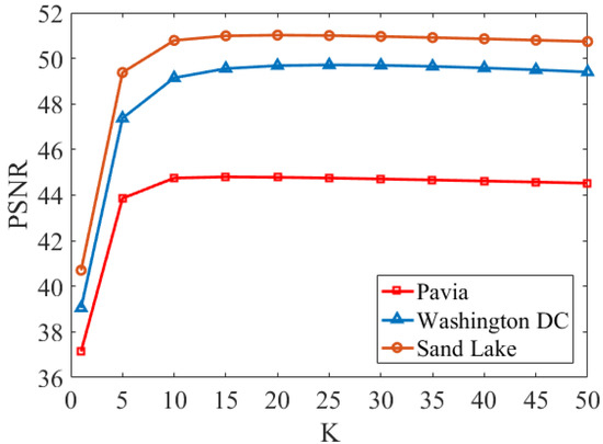
Figure 1.
PSNR values for different K.
The parameter is the weight of the proximal term in (12). For the evaluation of the influence of , we perform the method for different . Figure 2 presents the change of PSNR values of the fused HSIs of the three datasets with different values (the base of log is 10). In the experiments of this paper, we take the range of to be set to [−3, 0]. As is displayed in Figure 2, there is a rise trend of PSNR for all three datasets as varies from −3 to −1, reaches a maximum when equals −1, and decreases sharply when is greater than −1. Therefore, we set to −1, i.e., we take = 0.1 for all three datasets.
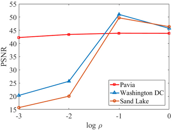
Figure 2.
PSNR values for different .
The regularization parameter in (10) controls the sparsity of the core tensor, therefore, affects the estimation of the HR-HSI. Higher values of yield sparser core tensor. Figure 3 shows the PSNR values of the reconstructed HSI for the Pavia University dataset under different . In this work, we set the range of to [−9, −2]. As shown in Figure 3, when belongs to [−9, −5], the PSNR stays relatively stable; when belongs to [−5, −4], the PSNR decreases slowly; and when > −4, the PSNR decreases sharply. Therefore, we set as −6, that is, for the Pavia University dataset. By the same token, the values for the Washington dataset and the Sand Lake dataset can be decided in the same way.
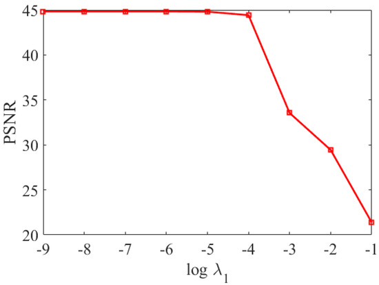
Figure 3.
PSNR values for different .
The unidirectional total variation regularization parameters , and control the segmental smoothness of the width-mode, height-mode and spectral-mode dictionaries, respectively. Figure 4 shows the reconstructed PSNR values of HSI for the Pavia University dataset with different , and . In the experiments of this paper, we set the range of values of and both to [−9, −2] and the range of values of to [−4, 4]. As shown in Figure 4 and Figure 5, the PSNR reaches its peak value when = −8, = −7, and = 2. Therefore, for Pavia University dataset, we set as −8, as −7, and as 2. It is worth noting that the optimal value of is relatively large compared of and , due to the fact that HSI is continuous in the spectral dimension, which leads to a potentially smaller full variation regularization of the dictionary along the spectral direction. Therefore, the optimal value of its regularization parameter should be relatively large. Similarly, the values of , and for the Washington and Sand Lake datasets can be determined in the same way.
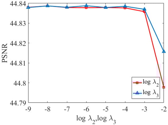
Figure 4.
PSNR values for different and .
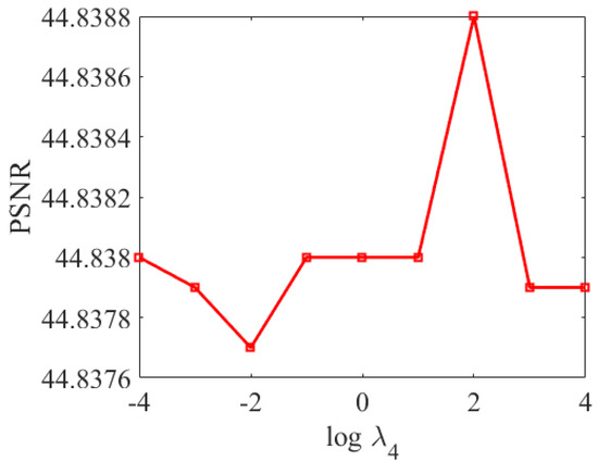
Figure 5.
PSNR values for different .
The graph regularization parameters and control the spectral structure of the spectral graph and the spatial correlation of the spatial graph, respectively. Figure 6 shows the reconstructed PSNR values of HSI for the Pavia University dataset under different and . In the experiments of this paper, we take the value range of both and to [−7, −1]. As shown in Figure 6, the PSNR reaches its peak value when and . Therefore, for the Pavia University dataset, we set as −1 and as −1. Similarly, the and values for the Washington dataset and the Sand Lake dataset can be determined in the same way.
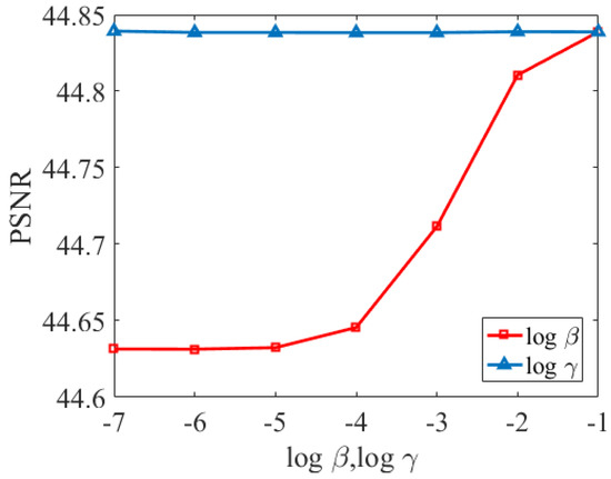
Figure 6.
PSNR values for different and .
The number of atoms in the three-model dictionaries are , and . Figure 7 shows the PSNR values of the fused HSI of the Pavia University dataset for different and , and Figure 8 shows the PSNR values of the fused HSI of the Pavia University dataset for different . In this paper, we set the range of values for both and to [260, 400], and set as [3, 21]. This is because the spectral features of HSI exist on the low-dimensional subspace. As shown in Figure 7, the PSNR increases sharply when is varied in the range [260, 360] and reaches a maximum at = 360, while it tends to decrease when is varied in the range [360, 400]. Therefore, we set as 360. It should be noted that the PSNR reaches its peak value when is 400, but what we have to consider is the overall performance of other evaluation indicators, so we set as 380 in the paper. It can be seen from Figure 8 that the PSNR decreases with > 15. Therefore, we set = 360, = 400, and = 15 for the Pavia University dataset. Similarly, the values of , and for the Washington dataset and the Sand Lake dataset can be determined in the same way.
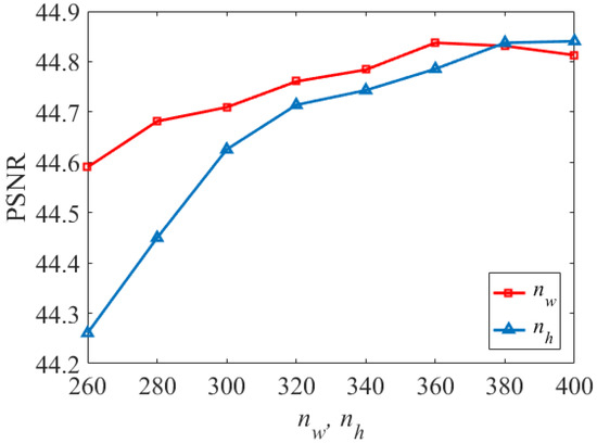
Figure 7.
PSNR values for different and .
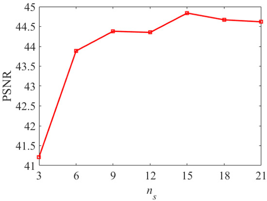
Figure 8.
PSNR values for different .
In Table 1, we give the tuning ranges for the 11 main parameters, give the values of each parameter for the three HSI datasets mentioned in Section 4.1, and show the recommended ranges for each parameter to easily tune the parameters.

Table 1.
Discussion of the main parameters.
4.5. Experimental Results
In this section, we show the fusion results of the five tested methods for the Pavia University, Washington DC, and Sand Lake datasets.
4.5.1. Experiment on Pavia University
In order to better display more spatial detail information and fusion results, we select three bands (R:61, G:25, B:13) to be synthesized as pseudo-color image for display, and then compared with other methods, the fusion results of Pavia University dataset are shown in the first row of Figure 9. In addition, to show the fusion performance more visually, we generate difference images to present the discrepancy between the reference image and the fused image. The second row in Figure 9 shows the difference image of the Pavia University dataset, which correspond to the fusion results in the first row.
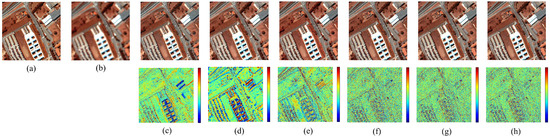
Figure 9.
Comparison of fusion results on the Pavia University dataset. (a) Reference Image; (b) LR-HSI; (c) CNMF; (d) HySure; (e) NLSTF; (f) CSTF; (g) UTV-HSISR; (h) JRLTD.
From Figure 9, we can see that the spatial details in the fusion results of different methods are greatly enhanced. However, compared with the reference image, there are still some spectral differences and noise effects in the fused image. For example, in Figure 9c,d, the fusion results of CNMF [29] and Hysure [18] show spectral distortion. Compared with the fusion results in Figure 9e,f, the fused images in Figure 9g,h are able to provide better spectral information and preserve the spatial structure.
In addition, it can be seen from the difference images that the reconstruction errors is relatively large from the difference images of Figure 9c–e. Figure 9g,h are better and similar compared with Figure 9f. In other words, the UTV-HSISR algorithm [41] and the JRLTD algorithm proposed in the paper achieve better fusion results, that is, there is little noise.
The quality indicators of the comparison method are shown in Table 2, and the better results obtained in the experiment are highlighted in bold typeface. From the spectral features, the algorithm proposed in this paper has the smallest RMSE, the closest CC to 1, the smallest ERGAS, the smallest SAM, and the smallest DD, indicating that the algorithm proposed in this paper is closest to the reference image, has the smallest spectral distortion, and has the best spectral agreement with the reference image. From the results of signal-to-noise ratio, the algorithm in this paper has the highest PSNR, which indicates that the algorithm has the best effective suppression of noise. From the spatial characteristics, SSIM is closest to 1, indicating that it is closest to the reference image in terms of brightness, contrast and structure; UIQI is closest to 1, indicating that the loss of relevant information reaches the minimum, the closer to the reference image.
Table 2.
Quality evaluation for Pavia University dataset.
4.5.2. Experiment on Washington DC
In order to better display more spatial detail information and fusion results, we select three bands(R:40, G:30, B:5) to be synthesized as pseudo-color image for display, and then compared with other methods, the fusion results of Washington DC dataset are shown in the first row of Figure 10. Besides, in order to show the fusion performance more visually, we generate difference images to present the discrepancy between the reference image and the fused image. The second row of Figure 10 shows the difference image of the Washington DC dataset.
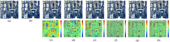
Figure 10.
Comparison of fusion results on the Washington DC dataset. (a) Reference Image; (b) LR-HSI; (c) CNMF; (d) HySure; (e) NLSTF; (f) CSTF; (g) UTV-HSISR; (h) JRLTD.
It can be seen that the spectral information is distorted in the results of CNMF [29] and HySure [18]. In addition, there are some blurring effects in the building regions in the results of NLSTF [38] when compared with Figure 10a. Compared with the fusion results of CSTF [39], the fused images of UTV-HSISR [41] and JRLTD are able to provide better spectral information and preserve the spatial structure. From the difference images, we can observe that the error of the UTV-HSISR algorithm [41] and the JRLTD algorithm proposed in the paper is smaller as a whole.
The quality evaluation results are shown in Table 3, and the better values obtained in the experiment are marked with bolded font. From Table 3, it can be seen that the algorithm proposed in this paper has the smallest RMSE, the closest CC to 1, the second minimum value of ERGAS, the smallest SAM, and the smallest DD in terms of spectral features. Collectively, the algorithm proposed in this paper is the closest to the reference image, with the smallest spectral distortion and the best spectral agreement with the reference image. From the results of signal-to-noise ratio, the algorithm in this paper has the highest PSNR, which indicates that the algorithm has the best effective suppression of noise. From the spatial characteristics, SSIM is closest to 1, which indicates that it is closest to the reference image in terms of brightness, contrast and structure; UIQI is closest to 1, which indicates that the loss of relevant information reaches the minimum, the closer to the reference image. In summary, the JRLTD algorithm proposed in this paper outperforms other algorithms in most cases.
Table 3.
Quality evaluation for Washington DC dataset.
4.5.3. Experiment on Sand Lake in Ningxia of China
In order to better display more spatial detail information and fusion results, we select three bands (R:41, G:25, B:3) to be synthesized as pseudo-color image for displaying, respectively, and then compared with other methods, the fusion results of Sand Lake dataset are shown in the first row of Figure 11. In addition, to show the fusion performance more visually, we generate difference images to present the discrepancy between the reference image and the fused image. The second row of Figure 11 shows the difference image of the Sand Lake dataset.
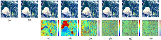
Figure 11.
Comparison of fusion results on the Sand Lake dataset. (a) Reference Image; (b) LR-HSI; (c) CNMF; (d) HySure; (e) NLSTF; (f) CSTF; (g) UTV-HSISR; (h) JRLTD.
After corresponding the fusion results obtained in the first row of Figure 11 using different algorithms with the difference images in the second row, we can see that Figure 11c–e have spectral distortion compared to the reference image. In addition, we can observe that the Figure 11c–e are poorly reconstructed, so the difference images seems to have a lot of information. From the difference images, Figure 11g,h are better and similar compared to Figure 11f. In other words, the UTV-HSISR algorithm [41] and the JRLTD algorithm proposed in the paper achieve better fusion results, that is, there is little noise.
Furthermore, Table 4 displays the quantitative experimental evaluations with eight metrics. The better values obtained in the experiment are indicated in bold. As can be seen from Table 4, from the spectral features, the algorithm proposed in this paper has the smallest RMSE, the smallest ERGAS, the smallest SAM, the smallest DD, and CC values are the same as those obtained by the UTV-HSISR algorithm. Overall, it shows that the algorithm proposed in this paper is closest to the reference image, has the smallest spectral distortion, and has the best spectral agreement with the source image. From the results of the signal-to-noise ratio, the algorithm in this paper has the highest PSNR, which indicates that the algorithm has the best effective suppression of noise. From the spatial characteristics, SSIM is closest to 1, which indicates that it is closest to the reference image in terms of brightness, contrast and structure; UIQI is closest to 1, which indicates that the loss of relevant information reaches the minimum, the closer to the reference image. In general, the JRLTD algorithm proposed in this paper outperforms other algorithms in most cases.
Table 4.
Quality evaluation for Sand Lake dataset.
5. Conclusions
In this paper, a hyperspectral image super-resolution method using joint regularization as prior information is proposed. Considering the geometric structures of LR-HSI and HR-MSI, two graphs are constructed to capture the spatial correlation of HR-MSI and the spectral similarity of LR-HSI. Then, the presence of anomalous noise values in the images was reduced by smoothing the LR-HSI and HR-MSI using unidirectional total variational regularization. In addition, an optimization algorithm based on PAO and ADMM is utilized to efficiently solve the fusion model. Finally, experiments were conducted on two benchmark datasets and one real dataset. Compared with some fusion methods such as CNMF [29], HySure [18], NLSTF [38], CSTF [39], and UTV-HSISR [41], this fusion method produces better spatial details and better preservation of the spectral structure due to the superiority of joint regularization and tensor decomposition.
However, there are still some limitations, and there is room for improvement of the proposed JRLTD algorithm. For example, the proposed JRLTD algorithm has a high computational complexity, and this leads to a relatively long running time. In our future work, we aim to extend the method in two directions. On the one hand, since the model utilizes the ADMM algorithm, although it is possible to divide a large complex problem into multiple smaller problems that can be solved simultaneously in a distributed manner, leads to an increase in computational effort and a decrease in computational speed. Therefore, we will try to find a closed form solution for each sub-problem. Alternatively, it can be accelerated by using parallel computing techniques. On the other hand, there is non-local spatial similarity in HSI, that is, there are duplicate or similar structures in the image, and when processing blocks of images, we can use information from surrounding blocks of images that are similar to them. This prior information has been shown to be valid for image super-resolution problems. Therefore, we will investigate the incorporation of non-local spatial similarity into the JRLTD method.
Author Contributions
Funding acquisition, W.B.; Validation, K.Q.; Writing—original draft, M.C.; Writing—review & editing, W.B. All authors have read and agreed to the published version of the manuscript.
Funding
This work is supported by the Natural Science Foundation of Ningxia Province of China (Project No. 2020AAC02028), the Natural Science Foundation of Ningxia Province of China (Project No. 2021AAC03179) and the Innovation Projects for Graduate Students of North Minzu University (Project No.YCX21080).
Acknowledgments
The authors would like to thank the Key Laboratory of Images and Graphics Intelligent Processing of State Ethnic Affairs Commission: IGIPLab for their support.
Conflicts of Interest
The authors declare no conflict of interest.
Abbreviations
| HSI-SR | Hyperspectral image super-resolution |
| LR-HSI | Low-resolution hyperspectral image |
| HR-MSI | High-resolution multispectral image |
| HR-HSI | High-resolution hyperspectral image |
| JRLTD | Joint regularized low-rank Tensor decomposition method |
| TV | Total variation |
| ADMM | Alternating direction multiplier method |
| PAO | Proximal alternate optimization |
| CNMF | Coupled non-negative matrix factorization |
| HySure | Hyperspectral image superresolution via subspace-based regularization |
| NLSTF | Non-local sparse tensor factorization |
| CSTF | Coupled sparse Tensor factorization |
| PSNR | Peak signal-to-noise ratio |
| ERGAS | Error relative global dimensionless synthesis |
| SAM | spectral angle mapping |
| RMSE | Root mean square error |
| CC | Correlation coefficient |
| DD | Distortion degree |
| SSIM | Structural similarity |
| UIQI | Universal image quality index |
Appendix A
Appendix A.1. Optimization of P 1
Problem (14) is convex and can be solved efficiently by ADMM. Thus, we introduce the variable and then the unconstrained optimization in (14) can be reexpressed as an equivalent constrained form, i.e.,
It is easy to deduce that the augmented Lagrangian function for problem (A1) is
where denotes the Lagrange multiplier and represents a positive penalty parameter. We solve (A2) using the ADMM algorithm:
(1) -Subproblem: From (A2), we have
The optimization problem in (A4) is quadratic, which has a unique solution, and it is equal to compute the following Sylvester matrix equation, i.e.,
We adopt the CG [46] to solve (A5) efficiently.
(2) M-Subproblem: From (A2), we have
Note that it is complicated to solve due to the Kronecker product involved in the regularization of the spatial graph. Taking advantage of the symmetry and positive-semidefinite of Laplacian matrices, we simplify formula (A6) by implementing the Cholesky factorization [49] of . After that, we obtain a more contextually specific and brief function with respect to M as
where is the matrix obtained by performing the Cholesky decomposition of and combining it with the Tucker2 decomposition model. The solution of the function (A7) can be obtained from the following equation:
where I denotes a unit matrix of appropriate size, .
(3) -Subproblem: From (A2), the Lagrangian multiplier can be updated by the following formula:
Specifically, the each step of solving -subproblem (13) by the ADMM is summarized in Algorithm A1.
| Algorithm A1 Solve -Subproblem (13) with ADMM. |
| Input: Y, Z, , , , , , , , , , , and . Output: Dictionary matrix .
|
Appendix A.2. Optimization of P2
Like problem (14), problem (16) can be solved efficiently with ADMM. Hence, we introduce the variable and then the unconstrained optimization in (16) can be rephrased into an equivalent constrained form, i.e.,
It is easy to deduce that the augmented Lagrangian function for problem (A10) is
where denotes the Lagrangian multiplier and represents a positive penalty parameter. We solve (A11) using the ADMM algorithm:
(1) -Subproblem: From (A11), we have
The optimization problem in (A13) is quadratic, which has a unique solution, and it is equal to compute the following Sylvester matrix equation, i.e.,
We adopt the CG to solve (A14) efficiently.
(2) N-Subproblem: From (A11), we have
Note that the same calculation of the Kronecker product is needed here, and we can use the method of solving for M to solve for the solution with respect to N.
(3) -Subproblem: From (A11), the Lagrangian multiplier can be updated by the following formula:
Specifically, the each step of solving -subproblem (15) by the ADMM is summarized in Algorithm A2.
| Algorithm A2 Solve -Subproblem (15) with ADMM. |
| Input: Y, Z, , , , , , , , , , , and . Output: Dictionary matrix .
|
Appendix A.3. Optimization of P3
Like problem (14), problem (18) can be solved efficiently with ADMM. Hence, we introduce the variable and then the unconstrained optimization in (18) can be rephrased into an equivalent constrained form, i.e.,
It is easy to deduce that the augmented Lagrangian function for problem (A17) is
where denotes the Lagrangian multiplier and represents a positive penalty parameter. We solve (A18) using the ADMM algorithm:
(1) -Subproblem: From (A18), we have
The optimization problem in (A20) is quadratic, which has a unique solution, and it is equal to compute the following Sylvester matrix equation, i.e.,
We adopt the CG to solve (A21) efficiently.
(2) O-Subproblem: From (A18), we have
After that, we obtain the closed solution of O:
where I denotes a unit matrix of appropriate size, .
(3) -Subproblem: From (A18), the Lagrangian multiplier can be updated by the following formula:
Specifically, the each step of solving -subproblem (17) by the ADMM is summarized in Algorithm A3.
| Algorithm A3 Solve -Subproblem (17) with ADMM. |
| Input: Y, Z, , , , , , , , , , , and . Output: Dictionary matrix .
|
Appendix A.4. Optimization of C
Problem (19) is convex and can be solved efficiently by ADMM algorithm by introducing two auxiliary variables and and then reformulate the problem (19) as follows:
where
It is easy to deduce that the augmented Lagrangian function for problem (A26) is
where , denotes the Lagrangian multiplier and represents a positive penalty parameter.
ADMM iterations of (A27) are shown below:
(1) -Subproblem: From (A27), we have
whose solution can be easily derived by columnwise vector-soft threshold function as:
where .
(2) -Subproblem: From (A27), we have
Problem (A31) is equal to
where the vectors , , and are generated by vectorizing the tensors , , and Y, respectively, and .
Problem (A32) has the following closed-form solution, i.e.,
Note that is extremely large, and formula in (A33) is complicated to solve. Fortunately, we find that
where and are diagonal matrices and unitary matrices containing the eigenvalues and eigenvectors of , , and , respectively.
Therefore, is a diagonal matrix and could be computed easily. Besides, the term in (A33) can be computed by
(3) -Subproblem: From (A27), we have
Problem (A36) is equal to
where the vectors , , and are generated by vectorizing the tensors , , and Z, respectively, and .
Problem (A37) has the following closed-form solution, i.e.,
Note that is extremely large, and formula in (A38) is complicated to solve. Fortunately, we find that
where and are diagonal matrices and unitary matrices containing the eigenvalues and eigenvectors of , , and , respectively.
Therefore, is a diagonal matrix and could be computed easily.
(3) and -Subproblem: From (A27), the multipliers and can be updated by the following formulas:
Specifically, the each step of solving -subproblem (19) by the ADMM is summarized in Algorithm A4.
| Algorithm A4 Solve - Subproblem (19) with ADMM. |
| Input: Y, Z, , , , , , , , , , and . Output: Core tensor .
|
References
- Bioucas-Dias, J.M.; Plaza, A.; Camps-Valls, G.; Scheunders, P.; Nasrabadi, N.; Chanussot, J. Hyperspectral remote sensing data analysis and future challenges. IEEE Geosci. Remote. Sens. Mag. 2013, 1, 6–36. [Google Scholar] [CrossRef] [Green Version]
- Vivone, G.; Alparone, L.; Chanussot, J.; Dalla Mura, M.; Garzelli, A.; Licciardi, G.A.; Restaino, R.; Wald, L. A critical comparison among pansharpening algorithms. IEEE Trans. Geosci. Remote. Sens. 2014, 53, 2565–2586. [Google Scholar] [CrossRef]
- Aiazzi, B.; Alparone, L.; Baronti, S.; Garzelli, A.; Selva, M. Years of pansharpening: A critical review and new developments. In Signal Image Processing for Remote Sensing, 2nd ed.; Chen, C.H., Ed.; CRC Press: Boca Raton, FL, USA, 2012; Volume 25, pp. 533–548. [Google Scholar]
- Meng, X.; Shen, H.; Li, H.; Zhang, L.; Fu, R. Review of the pansharpening methods for remote sensing images based on the idea of meta-analysis: Practical discussion and challenges. Inf. Fusion 2019, 46, 102–113. [Google Scholar] [CrossRef]
- Vivone, G.; Restaino, R.; Licciardi, G.; Dalla Mura, M.; Chanussot, J. Multiresolution analysis and component substitution techniques for hyperspectral pansharpening. In Proceedings of the 2014 IEEE Geoscience and Remote Sensing Symposium, Quebec City, QC, Canada, 13–18 July 2014; pp. 2649–2652. [Google Scholar]
- Kwarteng, P.; Chavez, A. Extracting spectral contrast in Landsat Thematic Mapper image data using selective principal component analysis. Photogramm. Eng. Remote Sens. 1989, 55, 339–348. [Google Scholar]
- Feng-Hua, H.; Lu-Ming, Y. Study on the hyperspectral image fusion based on the gram_schmidt improved algorithm. Inf. Technol. J. 2013, 12, 6694. [Google Scholar] [CrossRef]
- Alparone, L.; Baronti, S.; Aiazzi, B.; Garzelli, A. Spatial methods for multispectral pansharpening: Multiresolution analysis demystified. IEEE Trans. Geosci. Remote Sens. 2016, 54, 2563–2576. [Google Scholar] [CrossRef]
- Li, H.; Manjunath, B.; Mitra, S.K. Multisensor image fusion using the wavelet transform. Graph. Model. Image Process. 1995, 57, 235–245. [Google Scholar] [CrossRef]
- Liu, J. Smoothing filter-based intensity modulation: A spectral preserve image fusion technique for improving spatial details. Int. J. Remote Sens. 2000, 21, 3461–3472. [Google Scholar] [CrossRef]
- Aiazzi, B.; Alparone, L.; Baronti, S.; Garzelli, A.; Selva, M. MTF-tailored multiscale fusion of high-resolution MS and Pan imagery. Photogramm. Eng. Remote Sens. 2006, 72, 591–596. [Google Scholar] [CrossRef]
- Yuan, Q.; Wei, Y.; Meng, X.; Shen, H.; Zhang, L. A multiscale and multidepth convolutional neural network for remote sensing imagery pan-sharpening. IEEE J. Sel. Top. Appl. Earth Obs. Remote Sens. 2018, 11, 978–989. [Google Scholar] [CrossRef] [Green Version]
- Bungert, L.; Coomes, D.A.; Ehrhardt, M.J.; Rasch, J.; Reisenhofer, R.; Schönlieb, C.B. Blind image fusion for hyperspectral imaging with the directional total variation. Inverse Probl. 2018, 34, 044003. [Google Scholar] [CrossRef]
- Bajaj, C.; Wang, T. Blind Hyperspectral-Multispectral Image Fusion via Graph Laplacian Regularization. arXiv 2019, arXiv:1902.08224. [Google Scholar]
- Ghaderpour, E. Multichannel antileakage least-squares spectral analysis for seismic data regularization beyond aliasing. Acta Geophys. 2019, 67, 1349–1363. [Google Scholar] [CrossRef]
- Miao, J.; Cao, H.; Jin, X.B.; Ma, R.; Fei, X.; Niu, L. Joint sparse regularization for dictionary learning. Cogn. Comput. 2019, 11, 697–710. [Google Scholar] [CrossRef]
- He, Z.; Wang, Y.; Hu, J. Joint sparse and low-rank multitask learning with laplacian-like regularization for hyperspectral classification. Remote Sens. 2018, 10, 322. [Google Scholar] [CrossRef] [Green Version]
- Simoes, M.; Bioucas-Dias, J.; Almeida, L.B.; Chanussot, J. A convex formulation for hyperspectral image superresolution via subspace-based regularization. IEEE Trans. Geosci. Remote Sens. 2014, 53, 3373–3388. [Google Scholar] [CrossRef] [Green Version]
- Zhang, Y.; De Backer, S.; Scheunders, P. Noise-resistant wavelet-based Bayesian fusion of multispectral and hyperspectral images. IEEE Trans. Geosci. Remote Sens. 2009, 47, 3834–3843. [Google Scholar] [CrossRef]
- Akhtar, N.; Shafait, F.; Mian, A. Bayesian sparse representation for hyperspectral image super resolution. In Proceedings of the IEEE Conference on Computer Vision and Pattern Recognition, Boston, MA, USA, 7–12 June 2015; pp. 3631–3640. [Google Scholar]
- Ballester, C.; Caselles, V.; Igual, L.; Verdera, J.; Rougé, B. A variational model for P+ XS image fusion. Int. J. Comput. Vis. 2006, 69, 43–58. [Google Scholar] [CrossRef]
- Ning, M.; Ze-Ming, Z.; ZHANG, P.; Li-Min, L. A new variational model for panchromatic and multispectral image fusion. Acta Autom. Sin. 2013, 39, 179–187. [Google Scholar]
- Xing, Y.; Yang, S.; Feng, Z.; Jiao, L. Dual-Collaborative Fusion Model for Multispectral and Panchromatic Image Fusion. IEEE Trans. Geosci. Remote Sens. 2020, 1–15. [Google Scholar] [CrossRef]
- Zhu, X.X.; Bamler, R. A sparse image fusion algorithm with application to pan-sharpening. IEEE Trans. Geosci. Remote Sens. 2012, 51, 2827–2836. [Google Scholar] [CrossRef]
- Yang, X.; Jian, L.; Yan, B.; Liu, K.; Zhang, L.; Liu, Y. A sparse representation based pansharpening method. Future Gener. Comput. Syst. 2018, 88, 385–399. [Google Scholar] [CrossRef]
- Simsek, M.; Polat, E. Performance evaluation of pan-sharpening and dictionary learning methods for sparse representation of hyperspectral super-resolution. In Signal Image and Video Processing; Springer: Berlin/Heidelberg, Germany, 2021; pp. 1–8. [Google Scholar]
- Garzelli, A. A review of image fusion algorithms based on the super-resolution paradigm. Remote Sens. 2016, 8, 797. [Google Scholar] [CrossRef] [Green Version]
- Loncan, L.; De Almeida, L.B.; Bioucas-Dias, J.M.; Briottet, X.; Chanussot, J.; Dobigeon, N.; Fabre, S.; Liao, W.; Licciardi, G.A.; Simoes, M.; et al. Hyperspectral pansharpening: A review. IEEE Geosci. Remote Sens. Mag. 2015, 3, 27–46. [Google Scholar] [CrossRef] [Green Version]
- Yokoya, N.; Yairi, T.; Iwasaki, A. Coupled nonnegative matrix factorization unmixing for hyperspectral and multispectral data fusion. IEEE Trans. Geosci. Remote Sens. 2011, 50, 528–537. [Google Scholar] [CrossRef]
- Bioucas-Dias, J.M.; Plaza, A.; Dobigeon, N.; Parente, M.; Du, Q.; Gader, P.; Chanussot, J. Hyperspectral unmixing overview: Geometrical, statistical, and sparse regression-based approaches. IEEE J. Sel. Top. Appl. Earth Obs. Remote Sens. 2012, 5, 354–379. [Google Scholar] [CrossRef] [Green Version]
- Bendoumi, M.A.; He, M.; Mei, S. Hyperspectral image resolution enhancement using high-resolution multispectral image based on spectral unmixing. IEEE Trans. Geosci. Remote Sens. 2014, 52, 6574–6583. [Google Scholar] [CrossRef]
- Berné, O.; Helens, A.; Pilleri, P.; Joblin, C. Non-negative matrix factorization pansharpening of hyperspectral data: An application to mid-infrared astronomy. In Proceedings of the 2010 2nd Workshop on Hyperspectral Image and Signal Processing: Evolution in Remote Sensing, Reykjavik, Iceland, 14–16 June 2010; pp. 1–4. [Google Scholar]
- Kawakami, R.; Matsushita, Y.; Wright, J.; Ben-Ezra, M.; Tai, Y.W.; Ikeuchi, K. High-resolution hyperspectral imaging via matrix factorization. In Proceedings of the CVPR 2011, Colorado Springs, CO, USA, 20–25 June 2011; pp. 2329–2336. [Google Scholar]
- An, Z.; Shi, Z. Hyperspectral image fusion by multiplication of spectral constraint and NMF. Optik 2014, 125, 3150–3158. [Google Scholar] [CrossRef]
- Chen, Q.; Shi, Z.; An, Z. Hyperspectral image fusion based on sparse constraint NMF. Optik 2014, 125, 832–838. [Google Scholar] [CrossRef]
- Karoui, M.S.; Deville, Y.; Benhalouche, F.Z.; Boukerch, I. Hypersharpening by joint-criterion nonnegative matrix factorization. IEEE Trans. Geosci. Remote Sens. 2016, 55, 1660–1670. [Google Scholar] [CrossRef]
- Lanaras, C.; Baltsavias, E.; Schindler, K. Hyperspectral super-resolution by coupled spectral unmixing. In Proceedings of the IEEE International Conference on Computer Vision, Santiago, Chile, 7–13 December 2015; pp. 3586–3594. [Google Scholar]
- Dian, R.; Fang, L.; Li, S. Hyperspectral image super-resolution via non-local sparse tensor factorization. In Proceedings of the IEEE Conference on Computer Vision and Pattern Recognition, Honolulu, HI, USA, 21–26 June 2017; pp. 5344–5353. [Google Scholar]
- Li, S.; Dian, R.; Fang, L.; Bioucas-Dias, J.M. Fusing hyperspectral and multispectral images via coupled sparse tensor factorization. IEEE Trans. Image Process. 2018, 27, 4118–4130. [Google Scholar] [CrossRef]
- Zhang, K.; Wang, M.; Yang, S.; Jiao, L. Spatial–spectral-graph-regularized low-rank tensor decomposition for multispectral and hyperspectral image fusion. IEEE J. Sel. Top. Appl. Earth Obs. Remote Sens. 2018, 11, 1030–1040. [Google Scholar] [CrossRef]
- Xu, T.; Huang, T.Z.; Deng, L.J.; Zhao, X.L.; Huang, J. Hyperspectral image superresolution using unidirectional total variation with tucker decomposition. IEEE J. Sel. Top. Appl. Earth Obs. Remote Sens. 2020, 13, 4381–4398. [Google Scholar] [CrossRef]
- He, W.; Yokoya, N.; Yuan, L.; Zhao, Q. Remote sensing image reconstruction using tensor ring completion and total variation. IEEE Trans. Geosci. Remote Sens. 2019, 57, 8998–9009. [Google Scholar] [CrossRef]
- He, W.; Chen, Y.; Yokoya, N.; Li, C.; Zhao, Q. Hyperspectral super-resolution via coupled tensor ring factorization. arXiv 2020, arXiv:2001.01547. [Google Scholar]
- Xu, Y.; Wu, Z.; Chanussot, J.; Wei, Z. Hyperspectral images super-resolution via learning high-order coupled tensor ring representation. IEEE Trans. Neural Networks Learn. Syst. 2020, 31, 4747–4760. [Google Scholar] [CrossRef] [PubMed]
- Attouch, H.; Bolte, J.; Redont, P.; Soubeyran, A. Proximal alternating minimization and projection methods for nonconvex problems: An approach based on the Kurdyka-Łojasiewicz inequality. Math. Oper. Res. 2010, 35, 438–457. [Google Scholar] [CrossRef] [Green Version]
- Gene, H.; Van Loan, C. Matrix Computations; Johns Hopkins University Press: Baltimore, MD, USA, 2012; Volume 4. [Google Scholar]
- Smith, L.N.; Elad, M. Improving dictionary learning: Multiple dictionary updates and coefficient reuse. IEEE Signal Process. Lett. 2012, 20, 79–82. [Google Scholar] [CrossRef]
- Bioucas-Dias, J.M. A variable splitting augmented Lagrangian approach to linear spectral unmixing. In Proceedings of the 2009 First Workshop on Hyperspectral Image and Signal Processing: Evolution in Remote Sensing, Grenoble, France, 26–28 August 2009; pp. 1–4. [Google Scholar]
- Dereniowski, D.; Kubale, M. Cholesky factorization of matrices in parallel and ranking of graphs. In International Conference on Parallel Processing and Applied Mathematics; Springer: Berlin/Heidelberg, Germany, 2003; pp. 985–992. [Google Scholar]
Publisher’s Note: MDPI stays neutral with regard to jurisdictional claims in published maps and institutional affiliations. |
© 2021 by the authors. Licensee MDPI, Basel, Switzerland. This article is an open access article distributed under the terms and conditions of the Creative Commons Attribution (CC BY) license (https://creativecommons.org/licenses/by/4.0/).