1. Introduction
Hyperspectral images are obtained through hyperspectral sensors mounted on different platforms, which simultaneously image the target area in tens or even hundreds of consecutive and relatively narrow wavelength bands in multiple regions of the electromagnetic spectrum, such as the ultraviolet, visible, near-infrared and infrared, so it obtains rich spectral information along with surface image information. In other words, hyperspectral imagery combines image information and spectral information of the target area in one. The image information reflects the external characteristics such as size and shape of the sample, while the spectral information reflects the physical structure and chemical differences within the sample. In the field of hyperspectral image processing and applications, fusion [
1] is an important element. Furthermore, the problem of hyperspectral image super-resolution (HSI-SR) is to fuse the hyperspectral image (LR-HSI) with rich spectral information and poor spatial resolution with a multispectral image (HR-MSI) with less spectral information but higher spatial resolution to obtain a high-resolution hyperspectral image (HR-HSI). It can usually be divided into two categories: hyper-sharpening and MSI-HSI fusion.
The earliest work on hyper-sharpening was an extension of pansharpening [
2,
3]. Pan-sharpening is a fusion method that takes a high-resolution panchromatic (HR-PAN) image and a corresponding low-resolution multispectral (LR-MSI) image to create a high-resolution multispectral image (HR-MSI). Meng et al. [
4] first classified the existing pan-sharpening methods into component replacement (CS), multi-resolution analysis (MRA), and variational optimization (VO-based methods).
The steps of the CS [
5] based methods are to first project the MSI bands into a new space based spectral transform, after which the components representing the spatial information are replaced with HR-PAN images, and finally the fused images are obtained by back-projection. Representative methods include principal component analysis (PCA) [
6], Gram Schmidit (GS) [
7], etc. The multi-resolution analysis (MRA) [
8] method is a widely used method in pan-sharpening which is usually based on discrete wavelet transform (DWT) [
9]. The basic idea is to perform DWT on MS and Pan images, then retain the approximate coefficients in MSI and replace the spatial detail coefficients with the approximate coefficients of PAN images to obtain the fused images. Representative algorithms are smoothing filter-based intensity modulation (SFIM) [
10], generalized Laplace pyramid (GLP) [
11], etc. VO-based [
12] methods are an important class of pan-sharpening methods. Since the main fusion processes of regularization-based methods [
13,
14,
15,
16,
17], Bayesian-based methods [
18,
19,
20], model-based optimization (MBO) [
21,
22,
23] methods and sparse reconstruction (SR) [
24,
25,
26] based methods are all based on or transformed into an optimization of a variational model, they can be generalized to variational optimization (VO) based methods. In other words, the main process of such pan-sharpening methods is usually based on or transformed into an optimization of a variational model. A comprehensive review of VO methods based on the concept of super-resolution was first presented by Garzelli [
27]. As the availability of HS imaging systems increased, pan-sharpening was extended to HSI-SR by fusing HSI with PANs, which is referred to as hyper-sharpening [
28]. In addition, some hyper-sharpening methods have evolved from MSI-HSI fusion methods [
13,
14,
29]. In this case, MSI consists of only a single band, so MSI can be simplified to PAN images [
28], and a more detailed comparison of hyper-sharpening methods can be found in [
28].
In recent years, several methods have been proposed to realize the hyper-sharpening process of hyperspectral data, such as: linear spectral unmixing (LSU)-based techniques [
30,
31], nonnegative matrix decomposition-based methods [
29,
32,
33,
34,
35,
36,
37], tensor-based methods [
38,
39,
40,
41], and deep learning-based methods to improve the spatial resolution of hyperspectral data by using multispectral images. The LSU technique [
30] is essentially a problem of decomposing remote sensing data into endmembers and their corresponding abundances. Song et al. [
31] proposed a fast unmixing-based sharpening method, which uses unconstrained least squares algorithm to solve the endmember and abundance matrices. The innovation of the method is to apply the procedure to sub-images rather than to the whole data. Yokoya et al. [
29] proposed a nonnegative matrix factorization (NMF)-based hyper-sharpening algorithm called coupled NMF (CNMF) by alternately unmixing low-resolution HS data and high-resolution MS data. In CNMF, the endmember matrix and the abundance matrix are estimated using the alternating spectral decomposition of NMF under the constraints of the observation model. However, the results of CNMF may not always be satisfactory; firstly, the solution of NMF is usually non-unique, and secondly, its solution process is very time-consuming because it needs to continuously alternate the application of NMF unmixing to low spatial resolution hyperspectral and high spatial resolution multispectral data, which yields a hyperspectral endmember and a high spatial resolution abundance matrix. Later, by combining these two matrices, fused data with high spatial and spectral resolution can be obtained. An HSI-SR method based on the sparse matrix decomposition technique was proposed in [
33], which decomposes the HSI into a basis matrix and a sparse coefficient matrix. Then the HR-HSI was reconstructed using the spectral basis obtained from LR-HSI and the sparse coefficient matrix estimated by HR-MSI. Other NMF-based sharpening algorithms include spectral constraint NMF [
34], sparse constraint NMF [
35], joint-criterion NMF-based (JNMF) hyper-sharpening algorithm [
36], etc. Specifically, some of the NMF-based methods can also be applied to the fusion process of HS and PAN images, e.g., [
34,
35]. Furthermore, in order to obtain better fusion results, the work of [
37] exploited both the sparsity and non-negativity constraints of HR-HSI and achieved good performance.
Although many methods based on matrix decomposition under different constraints have been proposed by researchers and yielded better performance, these methods based on matrix decomposition require the three-dimensional remote sensing data to be expanded into the form of a two-dimensional matrix, which makes it difficult for the algorithms to take full advantage of the spatial spectral correlation of HSI. HSI-SR method based on tensor decomposition has become a hot topic in MSI-HSI fusion research because of its excellent performance. The main idea of its fusion is to treat HR-HSI as a three-dimensional tensor and to redefine the HSI-SR problem as the estimation of the core tensor and dictionary in three modes. Dian et al. [
38] first proposed a non-local sparse tensor factorization method for the HSI-SR problem (called NLSTF), which treats hyperspectral data as a tensor of three modes and combines the non-local similarity prior of hyperspectral images to nonlocally cluster MSI images, and although this method produced good results, LR-HSI was only used for learning the spectral dictionary and not for core tensor estimation. Li et al. [
39] proposed the coupled sparse tensor factorization (CSTF) method, which directly decomposes the target HR-HSI using Tucker decomposition and then promotes the sparsity of the core tensor using the high spatial spectral correlation in the target HR-HSI. In order to effectively preserve the spatial spectral structure in LR-HSI and HR-MSI, Zhang et al. [
40] proposed a new low-resolution HS (LRHS) and high-resolution MS (HRMS) image fusion method based on spatial–spectral-graph-regularized low-rank tensor decomposition (SSGLRTD). This method redefines the fusion problem as a low-rank tensor decomposition model by considering LR-HSI as the sum of HR-HSI and sparse difference images. Then, the spatial spectral low-rank features of HR-HSI images were explored using the Tucker decomposition method. Finally, the HR-MSI and LR-HSI images were used to construct spatial and spectral graphs, and regularization constraints were applied to the low-rank tensor decomposition model. Xu et al. [
41] proposed a new HSI-SR method based on a unidirectional total variational (TV) approach. The method has decomposed the target HR-HSI into a sparse core tensor multiplied by a three-mode dictionary matrix using Tucker decomposition, and then applied the
-norm to the core tensor to represent the sparsity of the target HR-HSI and the unidirectional TV three dictionaries to characterize the piecewise smoothness of the target HR-HSI. In addition, tensor ring-based super-resolution algorithms for hyperspectral images have recently attracted the attention of research scholars. He et al. [
42,
43] proposed a HSI-SR method based on a constrained tensor ring model, which decomposes the higher-order tensor into a series of three-dimensional tensors. Xu et al. [
44] proposed a super-resolution fusion of LR-HSI and HR-MSI using a higher-order tensor ring method, which preserves the spectral information and core tensor in a tensor ring to reconstruct high-resolution hyperspectral images.
Deep learning has received increasing attention in the field of HSI-SR with its superior learning performance and high speed. However, deep learning-based methods usually require a large number of samples to train the neural network to obtain the parameters of the network.
The Tucker tensor decomposition is a valid multilinear representation for high-dimensional tensor data, but it fails to take the manifold structures of high-dimensional HR-HSI into account. Furthermore, the graph regularization can perfectly preserve local information of high-dimensional data and achieve good performances in many fusion tasks. Moreover, the existing tensor decomposition-based methods are sensitive to outliers and noise, there is still much room for improvement. We propose a new method based on joint regularization low-rank tensor decomposition (JRLTD) in this paper to solve the HSI-SR problem from the tensor perspective. The model operates on hyperspectral data using the classical Tucker decomposition and introduces graph regularization and the unidirectional total variation regularization (TV), which effectively preserves the spatial and spectral structures in the fused hyperspectral images while reducing the presence of anomalous noise values in the images, thus solving the HSI-SR problem. The main contributions of the paper are summarized as follows.
- (1)
In the process of recovering high-resolution hyperspectral images (HR-HSI), joint regularization is considered to operate on the three-mode dictionary. The graph regularization can make full use of the manifold structure in LR-HSI and HR-MSI, while the unidirectional total variational regularization fully considers the segmental smoothness of the target image, and the combination of the two can effectively preserve the spatial structure information and the spectral structure information of HR-HSI.
- (2)
Based on the unidirectional total variational regularization, the -norm is used. The -norm is not only sparse for the sum of the absolute values of the matrix elements, but also requires row sparsity.
- (3)
During the experiments, not only the standard dataset of hyperspectral fusion is adopted, but also the dataset about the local Ningxia is used, which makes the algorithm more widely suitable and the performance more convincing.
The remainder of this paper is organized as follows.
Section 2 presents theoretical model and related work.
Section 3 describes the solution to the optimization model.
Section 4 describes our experimental results and evaluates the algorithm. Conclusions and future research directions are presented in
Section 5.
4. Experiments
4.1. Datasets
In this section, three datasets are used to test the performance of the proposed method.
The first dataset is the Pavia University dataset, which was acquired by the Italian Reflection Optical System Imaging Spectrometer (ROSIS) optical sensor in the downtown area of the University of Pavia. The image size is , with a spatial resolution of 1.3 m. We reduced the number of spectral bands to 93 after removing the water vapor absorption band. For reasons related to the down-sampling process, only the image in the upper left corner was used as a reference image in the experiment.
The second dataset is the Washington DC dataset, which is obtained from the Washington shopping mall acquired by the HYDICE sensor, intercepting images of size for annotation. The spatial resolution is 2.5m and contains a total of 210 bands. We intercept a part of the image with the size of for the experiment and use it as a reference image.
The third dataset is the Sand Lake in Ningxia of China, which is a scene acquired from the GF-5 AHSI sensor during the flight activity in Ningxia. The original image size is , its spatial resolution is 30 m, and the image has 330 bands, and the experiments reduce the spectral bands to 93 to obtain the reference image size of Sand Lake as .
4.2. Compared Algorithms
We selected classical and currently popular fusion methods for comparison, including CNMF [
29], HySure [
18], NLSTF [
38], CSTF [
39], and UTV-HSISR [
41]. The experiment was run on a PC equipped with an Intel Core i5-9300HF CPU, 16 GB RAM and NVIDIA GTX 1660Ti GPU. The Windows 10 x64 operating system was used and the programming application was Matlab R2016a.
4.3. Quantitative Metrics
For the evaluation of image fusion, it is more important to obtain more convincing values from objective metrics in addition to observing the results from subjective assumptions. To evaluate the fusion output in the numerical results, we use the following eight metrics, namely the peak signal-to-noise ratio (PSNR), which is an objective measure of image distortion or noise level; the error relative global dimensionless synthesis (ERGAS) to measure the comprehensive quality of the fused results; the spectral angle mapping (SAM) represents the absolute value of the spectral angle between two images; the root mean square error (RMSE) is used to measure the deviation between the predicted value and true value; the correlation coefficient (CC), which indicates the ability of the fused image to retain spectral information; the degree of distortion (DD), which is used to indicate the degree of distortion between the fused image and the ground truth image; the structural similarity (SSIM) and the universal image quality index (UIQI), which measures the degree of structural similarity between the two images.
The concept of mean squared deviation is first defined in the paper:
where
and
denote the size of the image,
I denotes a noise-free image, and
J denotes a noisy image. Then PSNR is defined as:
where
denotes the maximum number of pixels of the image. After that, the metrics we use to evaluate the fused image can be expressed by the following equation:
where
denotes the number of bands;
S denotes the spatial downsampling factor;
,
denote the value of the
ith band of the ground truth image and the fused image, respectively;
denotes the mean value of each band image;
denotes the mean pixel value of the original image;
is the mean pixel value of the fused image;
M denotes the sliding window;
,
denotes the mean value of
X,
, respectively;
,
denotes the standard deviation of
X,
, respectively;
,
are constants;
denotes the covariance of
,
. Furthermore,
,
denotes the variance of
,
, respectively. It should be noted that the best value of ERGAS, SAM, RMSE and DD is 0, the best value of CC, SSIM and UIQI is 1, and the best value of PSNR is
∞.
4.4. Parameters Discussion
JRLTD is mainly related to the following parameters, i.e., the number of PAO iterations K, the weights of the proximal terms , the sparse regularization parameters , the smooth regularization parameters , and , the graph regularization parameters and , and the number of three-mode dictionaries , and .
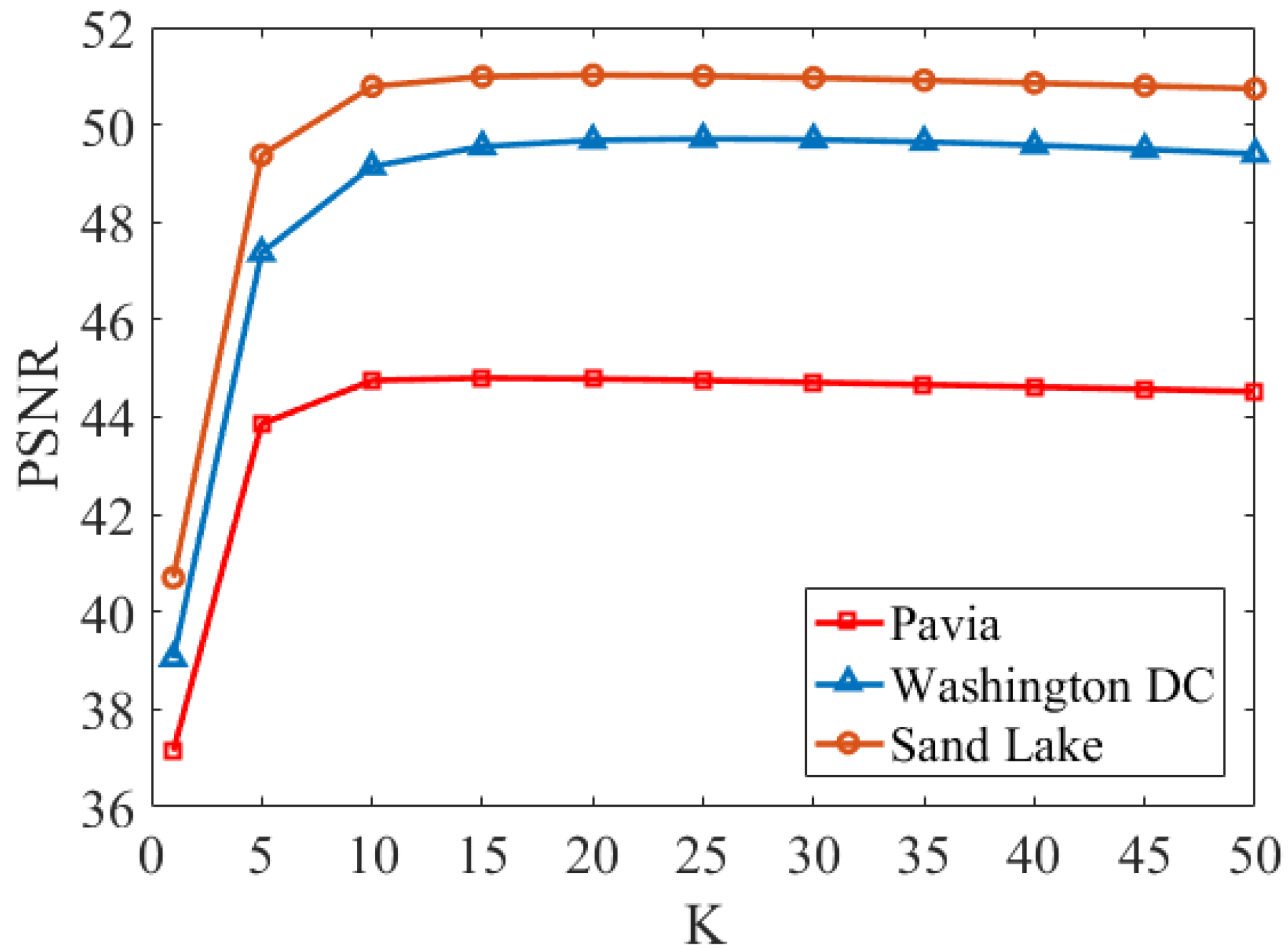
According to the description of Algorithm 1, we use the PAO scheme to solve the problem (10). The change of PSNR caused by the change in the number of PAO iterations
K is shown in
Figure 1. In
Figure 1, all three datasets show a fast increasing trend of PSNR as
K goes from 1 to 10. For the PAVIA dataset, there is a slight fluctuation in PSNR when
K varies from 10 to 50, and the maximum number of iterations of PAVIA is set to 20 in the experiment. The Washington dataset reached the maximum PSNR when
K = 25, so we set the maximum number of iterations of the algorithm in Washington to 25. Similarly, we set the maximum number of iterations for Sand Lake as 20.
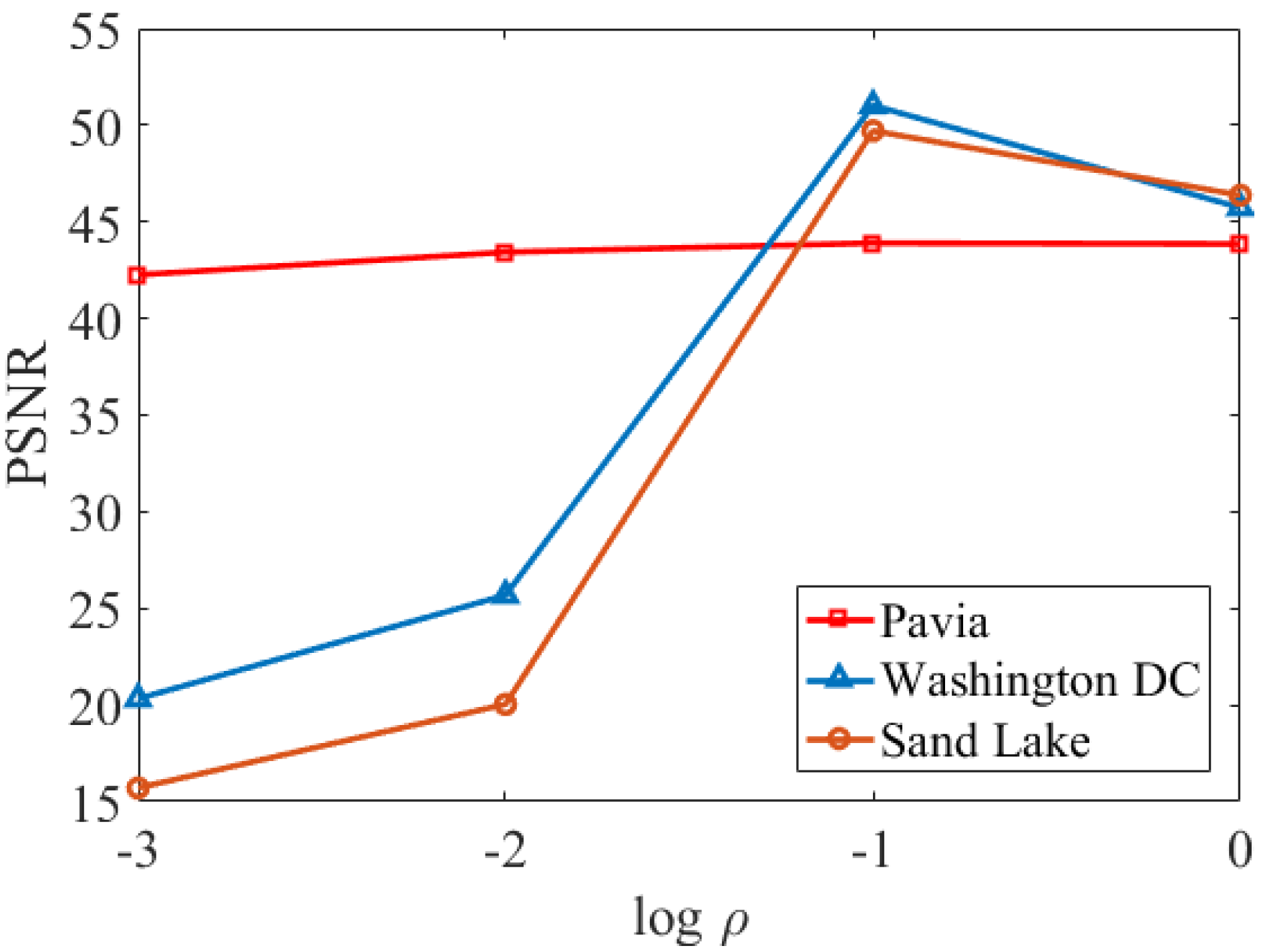
The parameter
is the weight of the proximal term in (12). For the evaluation of the influence of
, we perform the method for different
.
Figure 2 presents the change of PSNR values of the fused HSIs of the three datasets with different
values (the base of log is 10). In the experiments of this paper, we take the range of
to be set to [−3, 0]. As is displayed in
Figure 2, there is a rise trend of PSNR for all three datasets as
varies from −3 to −1, reaches a maximum when
equals −1, and decreases sharply when
is greater than −1. Therefore, we set
to −1, i.e., we take
= 0.1 for all three datasets.
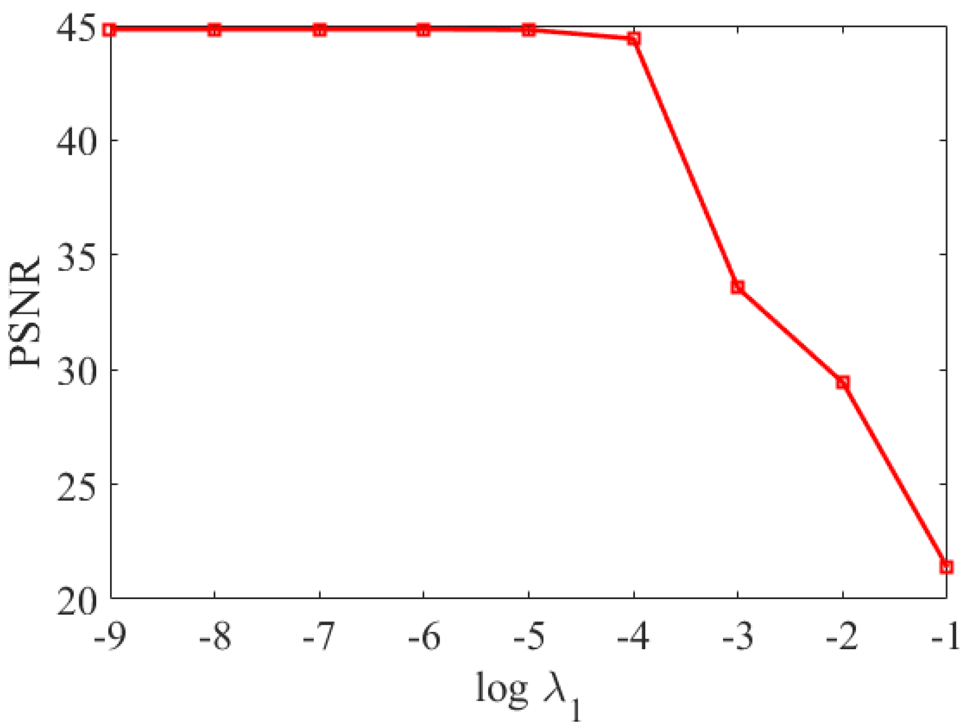
The regularization parameter
in (10) controls the sparsity of the core tensor, therefore,
affects the estimation of the HR-HSI. Higher values of
yield sparser core tensor.
Figure 3 shows the PSNR values of the reconstructed HSI for the Pavia University dataset under different
. In this work, we set the range
of to [−9, −2]. As shown in
Figure 3, when
belongs to [−9, −5], the PSNR stays relatively stable; when
belongs to [−5, −4], the PSNR decreases slowly; and when
> −4, the PSNR decreases sharply. Therefore, we set
as −6, that is,
for the Pavia University dataset. By the same token, the values for the Washington dataset and the Sand Lake dataset can be decided in the same way.
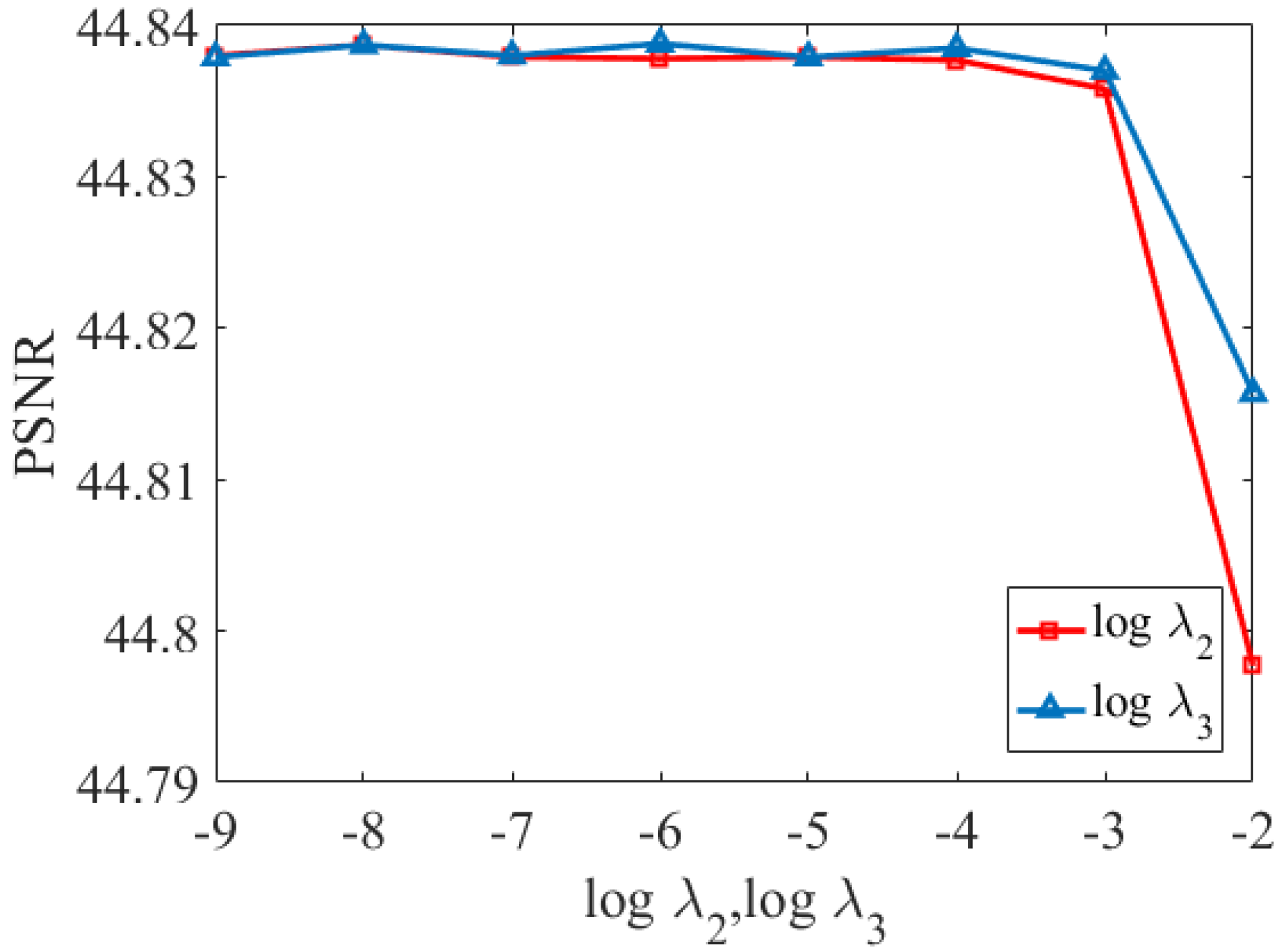
The unidirectional total variation regularization parameters
,
and
control the segmental smoothness of the width-mode, height-mode and spectral-mode dictionaries, respectively.
Figure 4 shows the reconstructed PSNR values of HSI for the Pavia University dataset with different
,
and
. In the experiments of this paper, we set the range of values of
and
both to [−9, −2] and the range of values of
to [−4, 4]. As shown in
Figure 4 and
Figure 5, the PSNR reaches its peak value when
= −8,
= −7, and
= 2. Therefore, for Pavia University dataset, we set
as −8,
as −7, and
as 2. It is worth noting that the optimal value of
is relatively large compared of
and
, due to the fact that HSI is continuous in the spectral dimension, which leads to a potentially smaller full variation regularization of the dictionary along the spectral direction. Therefore, the optimal value of its regularization parameter should be relatively large. Similarly, the values of
,
and
for the Washington and Sand Lake datasets can be determined in the same way.
The graph regularization parameters
and
control the spectral structure of the spectral graph and the spatial correlation of the spatial graph, respectively.
Figure 6 shows the reconstructed PSNR values of HSI for the Pavia University dataset under different
and
. In the experiments of this paper, we take the value range of both
and
to [−7, −1]. As shown in
Figure 6, the PSNR reaches its peak value when
and
. Therefore, for the Pavia University dataset, we set
as −1 and
as −1. Similarly, the
and
values for the Washington dataset and the Sand Lake dataset can be determined in the same way.
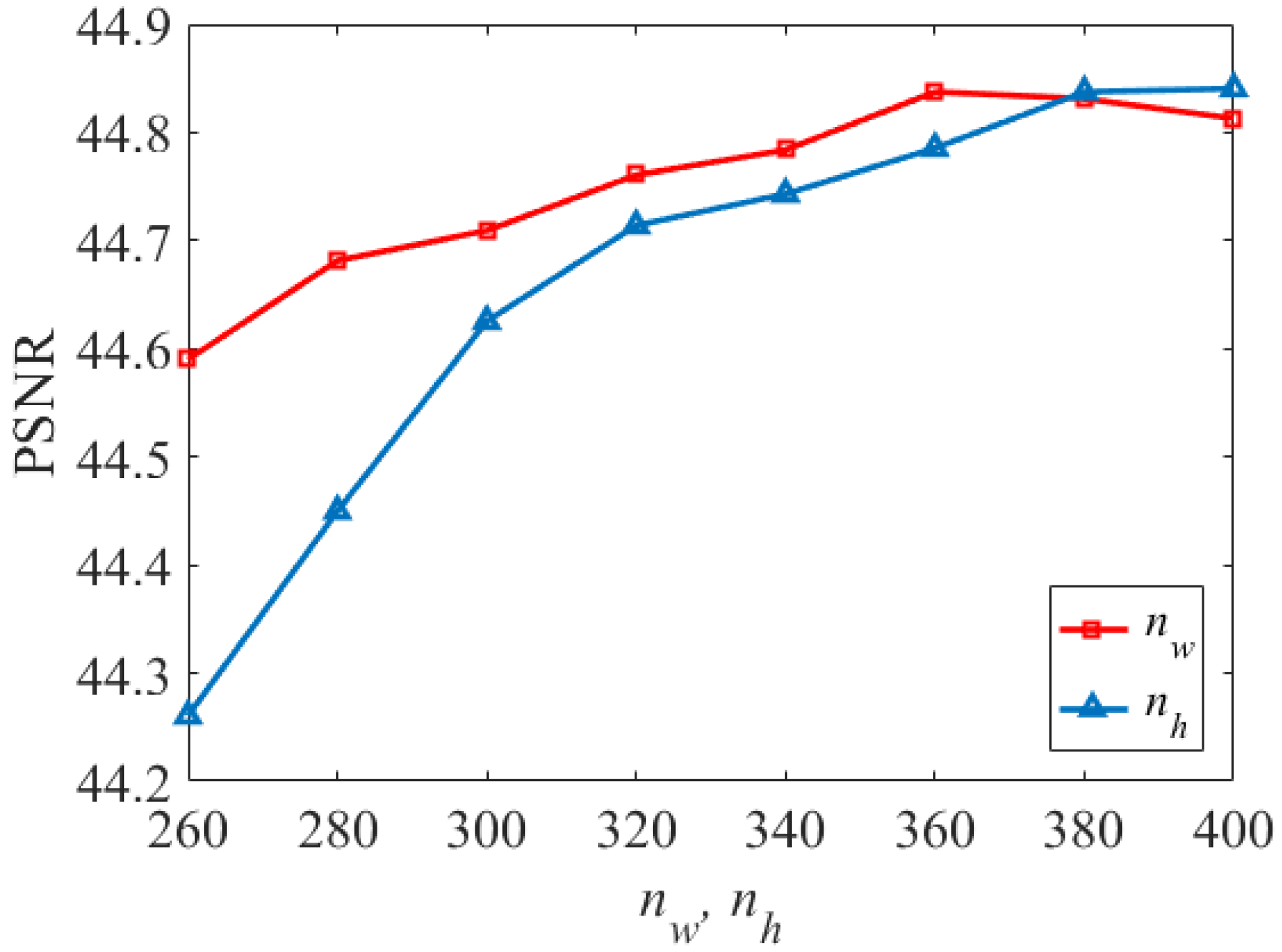
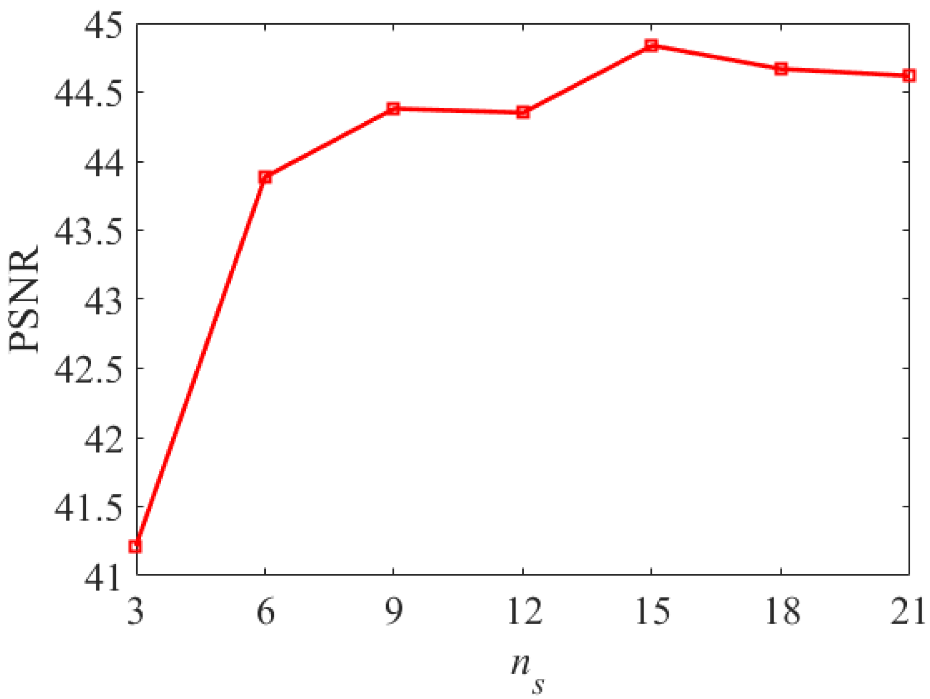
The number of atoms in the three-model dictionaries are
,
and
.
Figure 7 shows the PSNR values of the fused HSI of the Pavia University dataset for different
and
, and
Figure 8 shows the PSNR values of the fused HSI of the Pavia University dataset for different
. In this paper, we set the range of values for both
and
to [260, 400], and set
as [3, 21]. This is because the spectral features of HSI exist on the low-dimensional subspace. As shown in
Figure 7, the PSNR increases sharply when
is varied in the range [260, 360] and reaches a maximum at
= 360, while it tends to decrease when
is varied in the range [360, 400]. Therefore, we set
as 360. It should be noted that the PSNR reaches its peak value when
is 400, but what we have to consider is the overall performance of other evaluation indicators, so we set
as 380 in the paper. It can be seen from
Figure 8 that the PSNR decreases with
> 15. Therefore, we set
= 360,
= 400, and
= 15 for the Pavia University dataset. Similarly, the values of
,
and
for the Washington dataset and the Sand Lake dataset can be determined in the same way.
In
Table 1, we give the tuning ranges for the 11 main parameters, give the values of each parameter for the three HSI datasets mentioned in
Section 4.1, and show the recommended ranges for each parameter to easily tune the parameters.
4.5. Experimental Results
In this section, we show the fusion results of the five tested methods for the Pavia University, Washington DC, and Sand Lake datasets.
4.5.1. Experiment on Pavia University
In order to better display more spatial detail information and fusion results, we select three bands (R:61, G:25, B:13) to be synthesized as pseudo-color image for display, and then compared with other methods, the fusion results of Pavia University dataset are shown in the first row of
Figure 9. In addition, to show the fusion performance more visually, we generate difference images to present the discrepancy between the reference image and the fused image. The second row in
Figure 9 shows the difference image of the Pavia University dataset, which correspond to the fusion results in the first row.
From
Figure 9, we can see that the spatial details in the fusion results of different methods are greatly enhanced. However, compared with the reference image, there are still some spectral differences and noise effects in the fused image. For example, in
Figure 9c,d, the fusion results of CNMF [
29] and Hysure [
18] show spectral distortion. Compared with the fusion results in
Figure 9e,f, the fused images in
Figure 9g,h are able to provide better spectral information and preserve the spatial structure.
In addition, it can be seen from the difference images that the reconstruction errors is relatively large from the difference images of
Figure 9c–e.
Figure 9g,h are better and similar compared with
Figure 9f. In other words, the UTV-HSISR algorithm [
41] and the JRLTD algorithm proposed in the paper achieve better fusion results, that is, there is little noise.
The quality indicators of the comparison method are shown in
Table 2, and the better results obtained in the experiment are highlighted in bold typeface. From the spectral features, the algorithm proposed in this paper has the smallest RMSE, the closest CC to 1, the smallest ERGAS, the smallest SAM, and the smallest DD, indicating that the algorithm proposed in this paper is closest to the reference image, has the smallest spectral distortion, and has the best spectral agreement with the reference image. From the results of signal-to-noise ratio, the algorithm in this paper has the highest PSNR, which indicates that the algorithm has the best effective suppression of noise. From the spatial characteristics, SSIM is closest to 1, indicating that it is closest to the reference image in terms of brightness, contrast and structure; UIQI is closest to 1, indicating that the loss of relevant information reaches the minimum, the closer to the reference image.
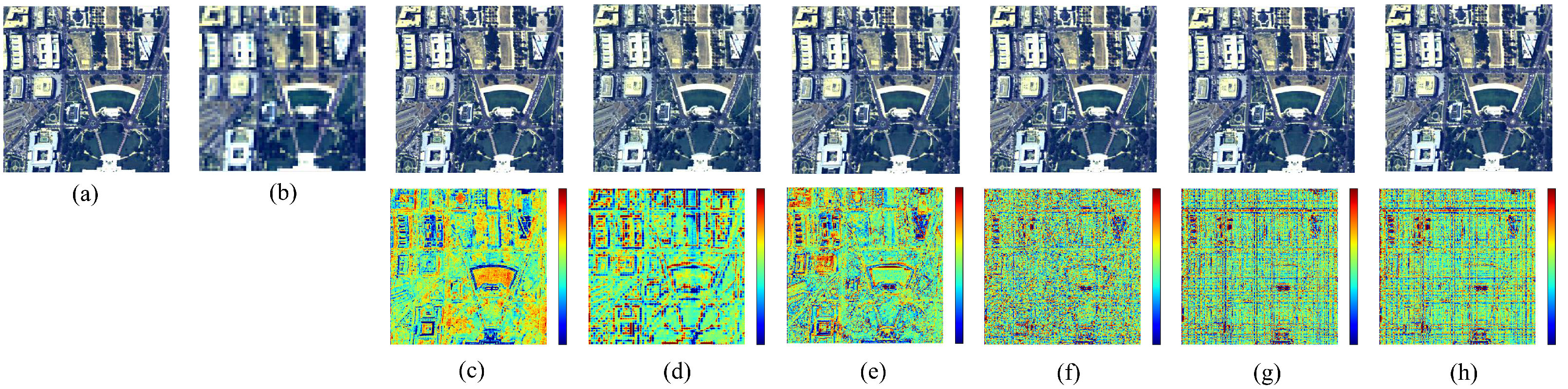
4.5.2. Experiment on Washington DC
In order to better display more spatial detail information and fusion results, we select three bands(R:40, G:30, B:5) to be synthesized as pseudo-color image for display, and then compared with other methods, the fusion results of Washington DC dataset are shown in the first row of
Figure 10. Besides, in order to show the fusion performance more visually, we generate difference images to present the discrepancy between the reference image and the fused image. The second row of
Figure 10 shows the difference image of the Washington DC dataset.
It can be seen that the spectral information is distorted in the results of CNMF [
29] and HySure [
18]. In addition, there are some blurring effects in the building regions in the results of NLSTF [
38] when compared with
Figure 10a. Compared with the fusion results of CSTF [
39], the fused images of UTV-HSISR [
41] and JRLTD are able to provide better spectral information and preserve the spatial structure. From the difference images, we can observe that the error of the UTV-HSISR algorithm [
41] and the JRLTD algorithm proposed in the paper is smaller as a whole.
The quality evaluation results are shown in
Table 3, and the better values obtained in the experiment are marked with bolded font. From
Table 3, it can be seen that the algorithm proposed in this paper has the smallest RMSE, the closest CC to 1, the second minimum value of ERGAS, the smallest SAM, and the smallest DD in terms of spectral features. Collectively, the algorithm proposed in this paper is the closest to the reference image, with the smallest spectral distortion and the best spectral agreement with the reference image. From the results of signal-to-noise ratio, the algorithm in this paper has the highest PSNR, which indicates that the algorithm has the best effective suppression of noise. From the spatial characteristics, SSIM is closest to 1, which indicates that it is closest to the reference image in terms of brightness, contrast and structure; UIQI is closest to 1, which indicates that the loss of relevant information reaches the minimum, the closer to the reference image. In summary, the JRLTD algorithm proposed in this paper outperforms other algorithms in most cases.
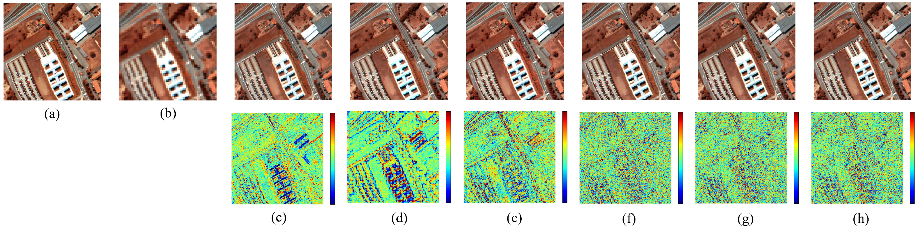
4.5.3. Experiment on Sand Lake in Ningxia of China
In order to better display more spatial detail information and fusion results, we select three bands (R:41, G:25, B:3) to be synthesized as pseudo-color image for displaying, respectively, and then compared with other methods, the fusion results of Sand Lake dataset are shown in the first row of
Figure 11. In addition, to show the fusion performance more visually, we generate difference images to present the discrepancy between the reference image and the fused image. The second row of
Figure 11 shows the difference image of the Sand Lake dataset.
After corresponding the fusion results obtained in the first row of
Figure 11 using different algorithms with the difference images in the second row, we can see that
Figure 11c–e have spectral distortion compared to the reference image. In addition, we can observe that the
Figure 11c–e are poorly reconstructed, so the difference images seems to have a lot of information. From the difference images,
Figure 11g,h are better and similar compared to
Figure 11f. In other words, the UTV-HSISR algorithm [
41] and the JRLTD algorithm proposed in the paper achieve better fusion results, that is, there is little noise.
Furthermore,
Table 4 displays the quantitative experimental evaluations with eight metrics. The better values obtained in the experiment are indicated in bold. As can be seen from
Table 4, from the spectral features, the algorithm proposed in this paper has the smallest RMSE, the smallest ERGAS, the smallest SAM, the smallest DD, and CC values are the same as those obtained by the UTV-HSISR algorithm. Overall, it shows that the algorithm proposed in this paper is closest to the reference image, has the smallest spectral distortion, and has the best spectral agreement with the source image. From the results of the signal-to-noise ratio, the algorithm in this paper has the highest PSNR, which indicates that the algorithm has the best effective suppression of noise. From the spatial characteristics, SSIM is closest to 1, which indicates that it is closest to the reference image in terms of brightness, contrast and structure; UIQI is closest to 1, which indicates that the loss of relevant information reaches the minimum, the closer to the reference image. In general, the JRLTD algorithm proposed in this paper outperforms other algorithms in most cases.
5. Conclusions
In this paper, a hyperspectral image super-resolution method using joint regularization as prior information is proposed. Considering the geometric structures of LR-HSI and HR-MSI, two graphs are constructed to capture the spatial correlation of HR-MSI and the spectral similarity of LR-HSI. Then, the presence of anomalous noise values in the images was reduced by smoothing the LR-HSI and HR-MSI using unidirectional total variational regularization. In addition, an optimization algorithm based on PAO and ADMM is utilized to efficiently solve the fusion model. Finally, experiments were conducted on two benchmark datasets and one real dataset. Compared with some fusion methods such as CNMF [
29], HySure [
18], NLSTF [
38], CSTF [
39], and UTV-HSISR [
41], this fusion method produces better spatial details and better preservation of the spectral structure due to the superiority of joint regularization and tensor decomposition.
However, there are still some limitations, and there is room for improvement of the proposed JRLTD algorithm. For example, the proposed JRLTD algorithm has a high computational complexity, and this leads to a relatively long running time. In our future work, we aim to extend the method in two directions. On the one hand, since the model utilizes the ADMM algorithm, although it is possible to divide a large complex problem into multiple smaller problems that can be solved simultaneously in a distributed manner, leads to an increase in computational effort and a decrease in computational speed. Therefore, we will try to find a closed form solution for each sub-problem. Alternatively, it can be accelerated by using parallel computing techniques. On the other hand, there is non-local spatial similarity in HSI, that is, there are duplicate or similar structures in the image, and when processing blocks of images, we can use information from surrounding blocks of images that are similar to them. This prior information has been shown to be valid for image super-resolution problems. Therefore, we will investigate the incorporation of non-local spatial similarity into the JRLTD method.


