Article

Optimal Vehicle Pose Estimation Network Based on Time Series and Spatial Tightness with 3D LiDARs

1
Hefei Institutes of Physical Science, Chinese Academy of Sciences, Hefei 230031, China
2
University of Science and Technology of China, Science Island Branch of Graduate School, Hefei 230026, China
3
Anhui Engineering Laboratory for Intelligent Driving Technology and Application, Hefei 230031, China
4
Innovation Research Institute of Robotics and Intelligent Manufacturing, Chinese Academy of Sciences, Hefei 230031, China
*
Author to whom correspondence should be addressed.
Remote Sens. 2021, 13(20), 4123; https://doi.org/10.3390/rs13204123
Submission received: 26 August 2021 / Revised: 6 October 2021 / Accepted: 7 October 2021 / Published: 14 October 2021

Abstract

:
Vehicle pose estimation is essential in autonomous vehicle (AV) perception technology. However, due to the different density distributions of the point cloud, it is challenging to achieve sensitive direction extraction based on 3D LiDAR by using the existing pose estimation methods. In this paper, an optimal vehicle pose estimation network based on time series and spatial tightness (TS-OVPE) is proposed. This network uses five pose estimation algorithms proposed as candidate solutions to select each obstacle vehicle’s optimal pose estimation result. Among these pose estimation algorithms, we first propose the Basic Line algorithm, which uses the road direction as the prior knowledge. Secondly, we propose improving principal component analysis based on point cloud distribution to conduct rotating principal component analysis (RPCA) and diagonal principal component analysis (DPCA) algorithms. Finally, we propose two global algorithms independent of the prior direction. We provided four evaluation indexes to transform each algorithm into a unified dimension. These evaluation indexes’ results were input into the ensemble learning network to obtain the optimal pose estimation results from the five proposed algorithms. The spatial dimension evaluation indexes reflected the tightness of the bounding box and the time dimension evaluation index reflected the coherence of the direction estimation. Since the network was indirectly trained through the evaluation index, it could be directly used on untrained LiDAR and showed a good pose estimation performance. Our approach was verified on the SemanticKITTI dataset and our urban environment dataset. Compared with the two mainstream algorithms, the polygon intersection over union (P-IoU) average increased by about 5.25% and 9.67%, the average heading error decreased by about 29.49% and 44.11%, and the average speed direction error decreased by about 3.85% and 46.70%. The experiment results showed that the ensemble learning network could effectively select the optimal pose estimation from the five abovementioned algorithms, making pose estimation more accurate.

1. Introduction

The continuous development of autonomous vehicles (AVs) has led to higher requirements for perception accuracy [1,2]. In perception technology, 3D object detection is one of its main research directions [3] that has received extensive attention from both industry and academia [4]. Although image-based 3D object detection has been significantly improved with the development of deep learning [5,6,7,8,9], it is difficult to provide accurate obstacle object depth information for images. Therefore, the access of depth information still relies on 3D point cloud data in actual applications [10].
Object detection based on the 3D point cloud falls into two categories: traditional methods and deep learning methods. In recent years, various deep learning methods [11,12] have continuously refreshed the detection accuracy rankings for the KITTI dataset [13]. However, these methods have still not been able to eliminate dependence on the dataset [14]. Better application effects necessitate ever-increasing reliance on the large-scale dataset.
In contrast, the adaptability of traditional methods is much better. In the traditional object detection pipeline of the 3D point cloud, it is generally necessary to first perform ground segmentation with the original point cloud [15] and then perform clustering processing with the point cloud data [16]. The object detection task is finally completed after estimating the pose of each obstacle according to the clustering results [17]. Its generalization performance is better for different hardware devices. As such, we were only interested in the obstacle vehicle pose estimation based on the 3D point cloud in this study.

1.1. Challenge of Pose Estimation

Although pose estimation is only a small part of the traditional 3D point cloud processing process, it is significant for the accuracy of object tracking algorithms because it is used as the input of the tracking algorithm [18]. The fluctuation error of pose estimation can cause the tracking algorithm to be unable to effectively track an obstacle’s trajectory. The fluctuation of pose estimation often depends on the distribution form of the obstacle 3D point cloud, which is fundamentally affected by the point cloud acquisition method.
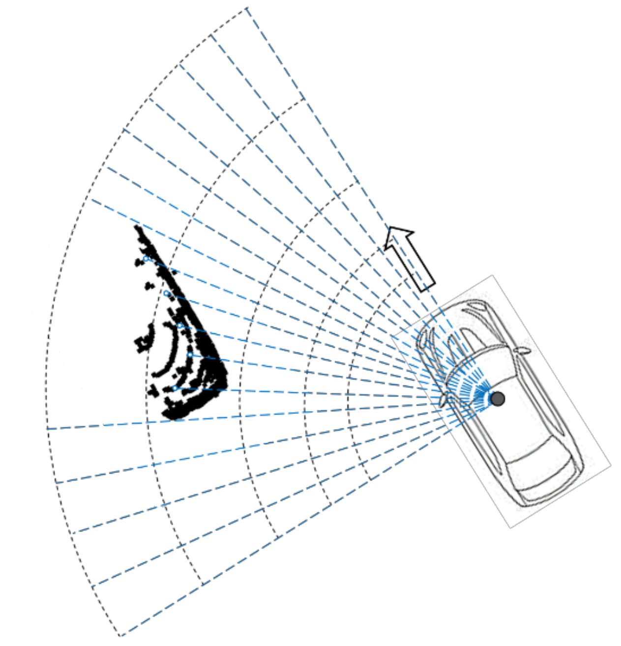
All point cloud data scanned by Light Detection and Ranging (LiDAR) are obtained by measuring the running time and position of the reflected light [19]. The observation time, angle, distance between vehicles, and mutual occlusion relationship change in real time during a vehicle’s driving [20,21,22], as shown in Figure 1. Therefore, obstacle vehicle pose estimation based on the 3D point cloud is still a challenging task.

1.2. Related Work

The current pose estimation algorithms for 3D point clouds based on traditional methods fall into two categories: pose estimation algorithms based on specific point cloud distribution shapes and global pose estimation algorithms.

1.2.1. Methods Based on Point Cloud Distribution Shapes

The pose estimation algorithms based on the distribution shape of a specific point cloud are generally classified into L-shape, I-shape, C-shape, and E-shape [23,24]. Since the L-shape has appeared most often in the distribution of 3D point clouds [25], many methods have used this feature to estimate the pose of obstacle vehicles. MacLachlan et al. [26] used the linear features of 3D point clouds to estimate the pose of obstacle vehicles. They first used the weighted least squares algorithm to remove outliers and proposed an obstacle pose estimation method using two linear features of straight-line fitting and right-angle fitting. The concept of the L-shape was not proposed in their article clearly. Still, the article was the beginning of L-shape pose estimation. Shen et al. [27] used point cloud scanning to iterate all possible corner points according to clockwise or counterclockwise timing characteristics. By incrementally constructing the problems and performing Eigen decomposition on the sub-matrix, the complexity could be reduced to as low as about nine times that of fitting a single pair of orthogonal lines. Following reductions of LiDAR price and the accuracy requirements of AVs [28], more and more vehicles have adopted multiple LiDAR splicing arrangements [29]. Zhang et al. [30] proposed an efficient search-based method for pose estimation to solve this problem; it relied on search-based algorithms to find the most suitable rectangle and then iterated all possible directions of the rectangle. Iteration enabled the authors to find the optimal direction via the minor square error of the rectangle containing all the scanning points in this direction, with which they fitted the rectangle. Qu et al. [31] also proposed a search-based L-shape pose estimation method that did not require a point cloud scanning sequence. They decomposed the L-shape fitting problem into two steps: L-shape vertex searching and L-shape corner point localizing. The three key points, which consisted of searched vertexes and localized the corner point, reflected the L-shape feature. Their algorithm [31] could effectively detect the best L-shape that fitted the 2D LiDAR data. Kim et al. [32] proposed an iterative endpoint fitting method to extract L-shape features from a 3D point cloud. They used the minimum and maximum clustering angle points as the endpoints of the baseline and iterated other point clouds as the breaking point. The final pose estimation bounding box was determined by extracting the farthest point from the baseline as the L-shaped corner point. These methods [31,32] were based on the assumption that all point clouds present a complete L-shape. In practice, due to occlusion and different viewing angles, a complete L-shape cannot be observed in most cases. As such, in [25], after selecting the approximate corner point, it was further judged whether the point was the corner point of the L-shape or the side point of the vehicle, and the RANSAC algorithm was used to fit the L-shape features to obtain pose estimation.
Although the abovementioned L-shape-based pose estimation methods can effectively utilize geometric features, they require that the point cloud presents an obvious L-shape. Additionally, when the point cloud number of obstacles is small, its geometric characteristics are not prominent and thus usually ignored. Therefore, the abovementioned L-shape-based pose estimation algorithms have poor global adaptability.

1.2.2. Methods Based on Global Algorithms

Compared to pose estimation based on a specific shape, a global-based pose estimation algorithm reduces dependence on the point cloud’s specific geometry and pays more attention to global applicability. Chen et al. [33,34] proposed a vehicle measurement model based on the likelihood-field-based model. The model was combined with a modified scaling series algorithm to estimate the pose of a target vehicle. However, when the point clouds were sparse, the particles’ randomness became strong, which reduced the accuracy of pose estimation. In response to this problem, Naujioks and Wuensche [35] proposed an algorithm that used a convex hull to make a preliminary estimate and a line-creation heuristic to fit a bounding box around incomplete segments of point clouds to correct vehicle orientation. This algorithm used the rapidity features of convex hull extraction, which could efficiently perform pose estimation even when the point cloud was sparse. Another idea to solve sparse point cloud distribution is the use of the coherent point drift pose estimation algorithm [36], which was one of the few pose estimation methods that used the object correlation algorithm to combine timing information. Although the algorithm fitted the vehicle measurement model well, the fitting randomness caused by the scaling series algorithm interfered with the pose estimation. An and Kim [18] proposed an algorithm for pose estimation using a low-end 3D LiDAR. The algorithm first established four obstacle vehicle models with different observation angles, then modeled the measured size of the object vehicle as a uniformly distributed sample, and finally used the idea of template matching to estimate the pose of the object vehicle. Yang et al. [17] proposed a vehicle pose estimation method based on edge distance, which used the bounding rectangle of the point cloud. After correcting the bounding box’s size according to the preset vehicle size, the pose estimation of the vehicle was finally completed. This method was more stable and easier to calculate compared to that of Kim et al. [18].
Although the abovementioned global-based pose estimation algorithms have better adaptability than L-shape-based pose estimation algorithms, they have poor pose estimation effects on curved road sections. Another significant problem is that, except for that of [36], no algorithms have considered the correlation between the front and rear frames of the obstacle, which means that when a frame had an obvious pose estimation error, it could not be effectively eliminated.

1.3. Overall of Our Approach

Based on our analysis, a new optimal vehicle pose estimation network based on time series and spatial tightness (TS-OVPE) is proposed in this paper. Figure 2 shows the pose estimation results of our approach.
The main contributions of this paper are summarized as follows.
  • We propose a new pose estimation network integrated with five potential pose estimation algorithms based on 3D LiDAR. This network was found to significantly improve the algorithm’s global adaptability and the sensitivity of direction estimation. It could also obtain an accurate performance on curved road sections.
  • We propose four evaluation indexes to reduce the pose estimation volatility between each frame. The four evaluation indexes are based on the spatial and time dimensions, and they allow for pose estimation that were found to be more robust and tighter other comparison methods.
  • We propose evaluation indexes to transform each algorithm into a unified dimension. The TS-OVPE network was indirectly trained with these evaluation indexes’ results. Therefore, they can be directly used on untrained LiDAR equipment and have good generalization performance.
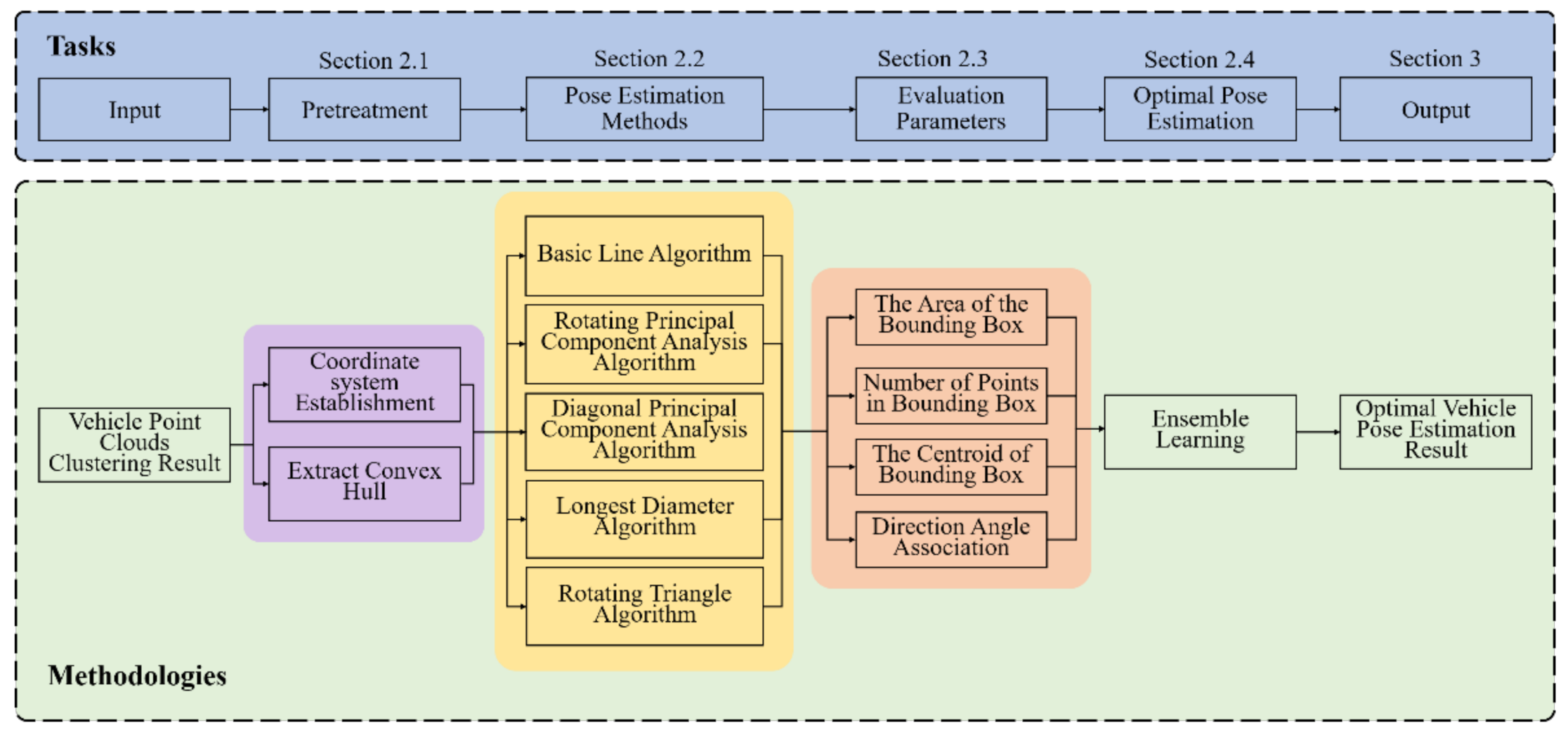
The remainder of this paper is organized as follows. In Section 2, the five pose estimation algorithms are proposed. Section 3 presents tests of the proposed algorithms in public and experimental datasets, as well as a discussion of the results. Finally, Section 4 summarizes the contribution of this paper and discusses future research directions. The flow chart of our approach is shown in Figure 3.

2. Methods

2.1. Pretreatment

Before obstacle pose estimation, this section first establishes the coordinate system used to facilitate calculations. Then, it introduces the concept of the convex hull to speed up computation and achieve real-time processing requirements.

2.1.1. Establishment of Coordinate System

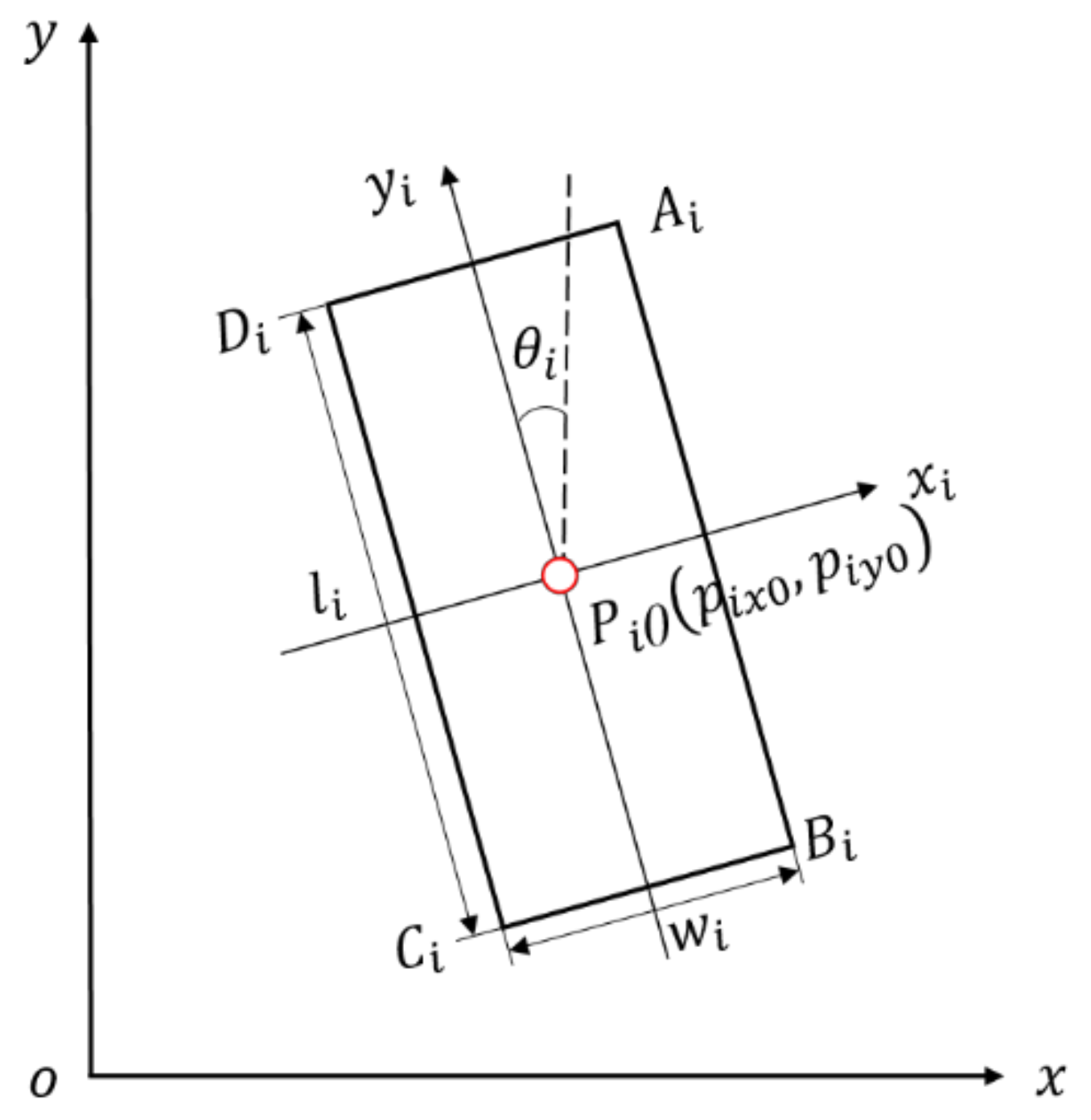
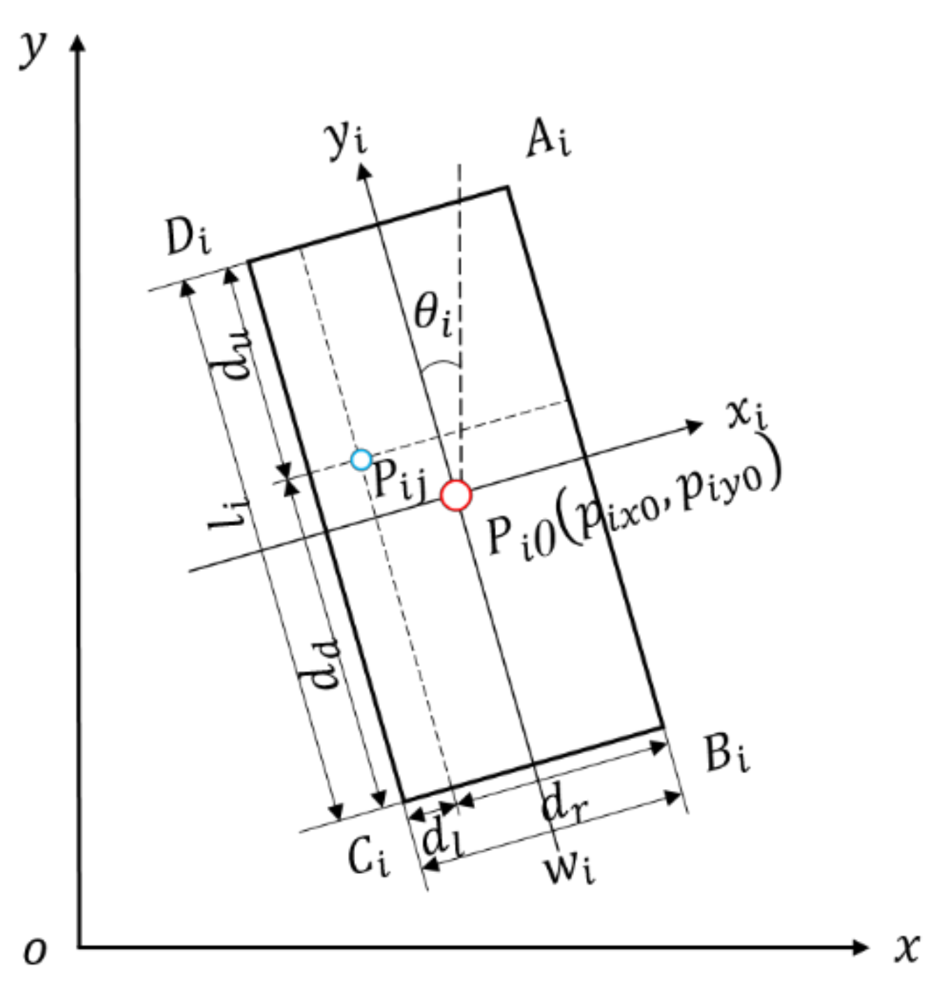
Any obstacle vehicle’s pose can be represented by a 3D bounding box. The 3D bounding box can reflect its driving direction information. The direction of the length side is the direction of the vehicle’s heading direction. When determining the 3D bounding box of an obstacle vehicle, eight vertices are generally used, but such description is redundant. The algorithm only needs the coordinates of four vertices of any horizontal cross section rectangle and adds height information; then, a 3D bounding box can be described. Therefore, our approach uses a two-dimensional plane coordinate system for each obstacle vehicle to describe its pose, as shown in Figure 4.
For the i obstacle vehicle, its pose can be represented by a vector p i :
p i = p i x 0 , p i y 0 , θ i , l i , w i , h i T
where p i x 0 and p i y 0 are the coordinates of the geometric center point of the i obstacle vehicle; θ i is the angle between its heading and the y direction; l i and w i are the length and width, respectively, of the obstacle; and h i is the height of the obstacle vehicle.
Vector p i can simplify the number of parameters in solving the obstacle pose. It can also express the four corners of the bounding box of the obstacle vehicle in the two-dimensional plane. A description of the bounding box corners A i , B i , C i , and D i is shown in Equation (2).
A i x B i x C i x D i x A i y B i y C i y D i y = cos θ i sin θ i sin θ i cos θ i p i x 0 + w i 2 p i x 0 + w i 2 p i x 0 w i 2 p i x 0 w i 2 p i y 0 + l i 2 p i y 0 l i 2 p i y 0 l i 2 p i y 0 + l i 2

2.1.2. Extraction of Convex Hull

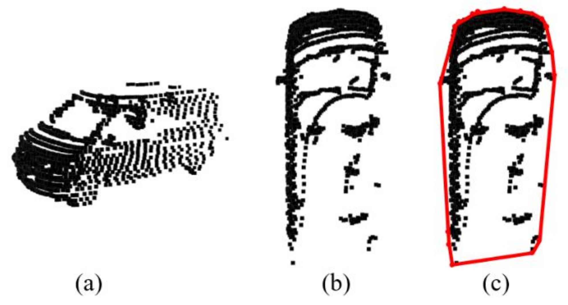
In point cloud data, each obstacle vehicle is composed of multiple point clouds. Figure 5 shows the original point cloud data of an obstacle vehicle. After projecting all the obstacle vehicle’s point clouds onto the horizontal plane, the projected points’ geometric contour can also genuinely reflect the obstacle vehicle’s geometric information. Analyzing the points inside its geometric contour is a meaningless waste of computing time. Therefore, our approach extracts its external contour from the point cloud’s convex hull before pose estimation.
The convex hull of an obstacle point cloud refers to the smallest convex polygon that enables all point clouds to be inside or on the convex hull. The extraction of the convex hull adopts the global convex hull algorithm proposed in [37]. On the premise of ensuring that the information is not lost, the invalid point cloud of each obstacle vehicle is reduced, which is economical in both computing space and time.

2.2. Vehicle Pose Estimation

In this section, we focus on the direction extraction of the bounding box. Our approach uses the road direction as a priori knowledge and improves the pose estimation algorithm based on principal component analysis (PCA). Furthermore, we propose two global algorithms independent of the prior direction.

2.2.1. Basic Line Algorithm

In the pose estimation of various obstacle vehicles, direction information is often ignored. While a vehicle is driving, its direction is mainly along the road, and road direction is very useful for pose estimation.
Our algorithm assumes that the directions of all obstacle vehicles are parallel or perpendicular to the road direction. Therefore, our approach only needs to find the extreme points in the x- and the y-directions after convex hull extraction, as shown in Figure 6. Although this algorithm is simple, its pose estimation effect is very advantageous in straight roads. Therefore, this algorithm is called the Basic Line algorithm. If a vehicle is driving on a curved road section, the directions are no longer vertical or horizontal and this method is longer applicable.

2.2.2. Pose Estimation Algorithms Based on PCA

Our analysis suggests that the estimation of the direction is a vital step. The authors of [38] used PCA to analyze the driving direction of obstacle point clouds; their results were not satisfactory, but the method was still reasonable from the perspective of theoretical analysis. Therefore, the authors of this paper explored the PCA method to improve direction extraction accuracy and performance in actual engineering applications.
  • Basic principles and feasibility analysis of PCA
The PCA method is used to map the multi-dimensional feature vector of original data from high-dimensional space to low-dimensional space through linear orthogonal transformations in order to obtain a set of linearly uncorrelated vectors of each dimension. PCA removes the correlation between dimensions and achieves dimensionality reduction. In the dimensionality reduction of the data in the x and y directions, PCA makes the final one-dimensional data variance as large as possible. The eigenvector corresponding to the largest eigenvalue of the covariance matrix is the driving direction of the vehicle.
The convex hull point set H = p i 1 , p i 2 , , p i n contains n convex hull points for the i obstacle vehicle in each frame of point cloud data. First, our approach first composes the point set H into a matrix H ¯ with two rows and n columns, where the first line of the matrix represents the x value of each point in the point set H and the second line represents the y value of the corresponding point, as shown in Equation (3).
H ¯ = p i 1 x p i 2 x p i 3 x p i n x p i 1 y p i 2 y p i 3 y p i n y
Second, our approach performs zero-average processing on the formed matrix H ¯ , calculates the mean values of all points in the x and y directions with Equation (4), and obtains the matrix H ¯ ’s zero averaging matrices with Equation (5). The zero averaging matrices are shown in Equation (6).
p i x ¯ = j = 1 n p i j x n p i y ¯ = j = 1 n p i j y n
p i j x = p i j x p i x ¯ p i j y = p i j y p i y ¯
Y = p i 1 x p i 2 x p i 3 x p i n x p i 1 y p i 2 y p i 3 y p i n y
Third, the covariance matrix C can be obtained with Equation (7).
C = 1 n Y Y T = 1 n p i 1 x p i 2 x p i 3 x p i n x p i 1 y p i 2 y p i 3 y p i n y p i 1 x p i 1 y p i 2 x p i 2 y p i 3 x p i 3 y p i n x p i n y
According to C - λ E = 0 , the eigenvalues λ 1 and λ 2 of the covariance matrix C can be solved. The corresponding feature vectors are c 1 = c 11 c 12 and c 2 = c 21 c 22 . Compare the larger λ max of the eigenvalues of λ 1 and λ 2 : the corresponding eigenvector is c max = c max 1 c max 2 . The feature vector c max represents the direction vector of the obstacle vehicle obtained by the PCA. Finally, the heading θ of the obstacle vehicle can be obtained with Equation (8).
θ = arctan c max 2 c max 1
When the obtained point cloud data of the obstacle vehicle are relatively complete, as shown in Figure 7a, the direction obtained by the PCA method is the driving direction of the obstacle vehicle. However, the point cloud of most obstacle vehicles is incomplete, as shown in Figure 7b. Because the scanned point cloud is missing diagonally, the direction obtained by PCA is the diagonal direction of the obstacle vehicle, not the obstacle vehicle’s forward direction. This is why the authors of [38] could not obtain satisfactory pose estimation results.
Therefore, we propose two pose estimation algorithms based on the direction characteristics obtained by PCA. The rotating principal component analysis (RPCA) algorithm is used for extracting obstacle vehicle’s driving directions. The diagonal principal component analysis (DPCA) algorithm used is for the extracting the obstacle vehicle’s diagonal directions. Detailed descriptions of these two algorithms are as follows.
  • Rotating Principal Component Analysis Algorithm
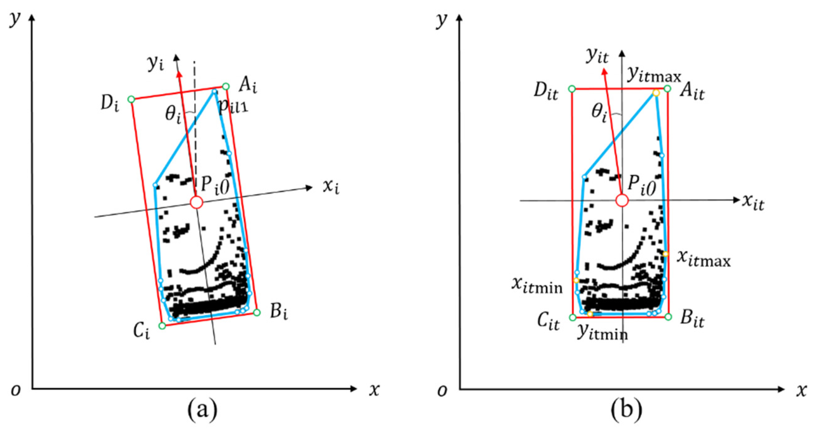
We designed the RPCA pose estimation algorithm by focusing on the situation shown in Figure 7a, in which the direction obtained by the PCA method is close to the driving direction of the obstacle vehicle. An error between y i (the actual direction of the vehicle) and the red arrow (the direction obtained by PCA) is present but minimal, so it can be ignored. Therefore, our approach assumes that the θ i obtained by the PCA is the actual driving direction.
For any point p i x i , y i in the x i p i 0 y i coordinate system, take point p i 0 as the center coordinate; then, according to the forward rotation Equation (9), rotate it θ i degrees clockwise in the y i direction (clockwise while θ i > 0 and counterclockwise while θ i < 0 ) to get p i x i t , y i t under the coordinate system x i t p i 0 y i t .
x i t y i t = cos θ i sin θ i sin θ i cos θ i x i x i
Furthermore, A i t , B i t , C i t , and D i t can be calculated after finding the extreme points of the x- and y-directions in the x i t p i 0 y i t coordinate system. According to the reverse rotation Equation (10), all points in the x i t p i 0 y i t coordinate system are rotated θ i and transformed back to the x i p i 0 y i coordinate system, as shown in Figure 8.
x i y i = cos θ i sin θ i sin θ i cos θ i x i t y i t
As a result, the corner point of the two-dimensional bounding box can be obtained in the original coordinate system x i p i 0 y i , as shown in Figure 8b.
  • Diagonal Principal Component Analysis Algorithm
The obstacle vehicle and own vehicle are sometimes in a relatively diagonal position, as shown in Figure 9. The point clouds of vehicles are relatively complete along their diagonal halves, and this asymmetry affects the PCA’s dimensionality reduction process. In this algorithm, our approach assumes the direction obtained by the PCA is the diagonal direction of the obstacle. Therefore, this algorithm is called the DPCA algorithm.
The convex hull point set H = p i 1 , p i 2 , , p i n contains n convex hull points for the i obstacle vehicle in each frame of point cloud data. First, it traverses any two points p k and p l in the convex hull point set H and calculates the straight-line p k p l ’s angle θ p between the y i direction. The difference between angles θ p and θ i obtained by the PCA is θ d . Then, the algorithm needs to find the two endpoints p k and p l as a set of diagonal points of the two-dimensional bounding box. The line p k p l first needs to have the closest direction to that extracted by the PCA, which requires following the smallest θ d . Moreover, the line p k p l needs to have the longest distance in this direction. Secondly, the algorithm finds the furthest point p f of the straight line p k p l in the convex hull point set H . After finding p k , p l , and p f , according to the rectangular character geometry, the two-dimensional bounding box of the initial obstacle vehicle is obtained, as shown in Figure 10.
The abovementioned algorithm was established under ideal conditions, but the four corners of a vehicle are mainly arc-shaped in actual point clouds. The diagonal points found in our study were not the real diagonal points of a bounding box. As shown in Figure 10, the obtained bounding box A i B i C i D i only contained a part of the point cloud, but its direction was consistent with the actual obstacle vehicle’s direction. Therefore, the bounding box needed to be fixed. According to the obtained direction, the extreme longitudinal points y i max and y i min in this direction and the extreme transverse points x i max and x i min perpendicular to this direction could be obtained. Figure 10 shows that the fixed bounding box A i * B i * C i * D i had a more accurate enclosing effect.

2.2.3. Longest Diameter Algorithm

The abovementioned pose estimation algorithms were mainly designed from the perspective of obstacle directions. We sought a better overall pose estimation method to put aside the dependence on PCA. Therefore, we proposed the Longest Diameter (LD) algorithm. Our LD algorithm could find the diagonal of an obstacle vehicle without direct guidance.
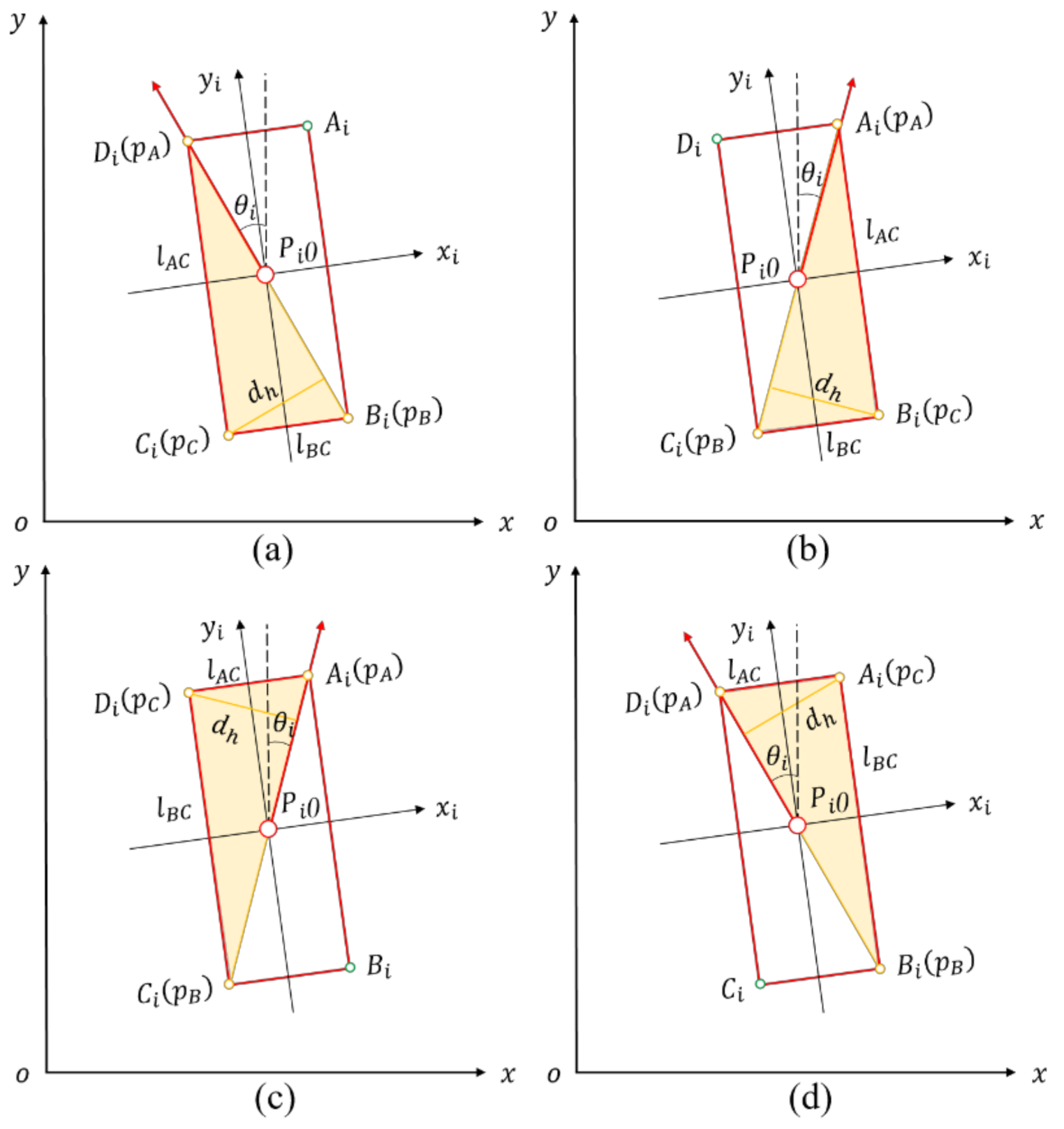
The LD algorithm calculates the obstacle vehicle’s two-dimensional bounding box when the two diagonal points have the longest distance and the farthest point of this line is located. Due to the different relative positions of vehicles, the diagonal direction of the obstacle may be left or right. Furthermore, the position of the third point, which is farthest from the diagonal, also appears in two different situations—on the left side or the right side of the diagonal line. The three points p A , p B , and p C have four different positional relationships, which are shown in Figure 11.
For the i obstacle vehicle in each frame of point cloud data, its convex hull point set H contains n convex hull points H = p i 1 , p i 2 , , p i n . Firstly, following the iteration of any two points in the convex hull point set H , the longest diameter of the convex hull is found. Secondly, the two points p A and p B with the longest distance in the diameter direction are diagonal points of the two-dimensional bounding box. Point p C is the furthest point from the straight line p A p B formed by these two points in the convex hull point set H . Following their identification, p A , p B , and p C also need to be adjusted with the Correction function to obtain the final pose estimation result.

2.2.4. Rotating Triangle Algorithm

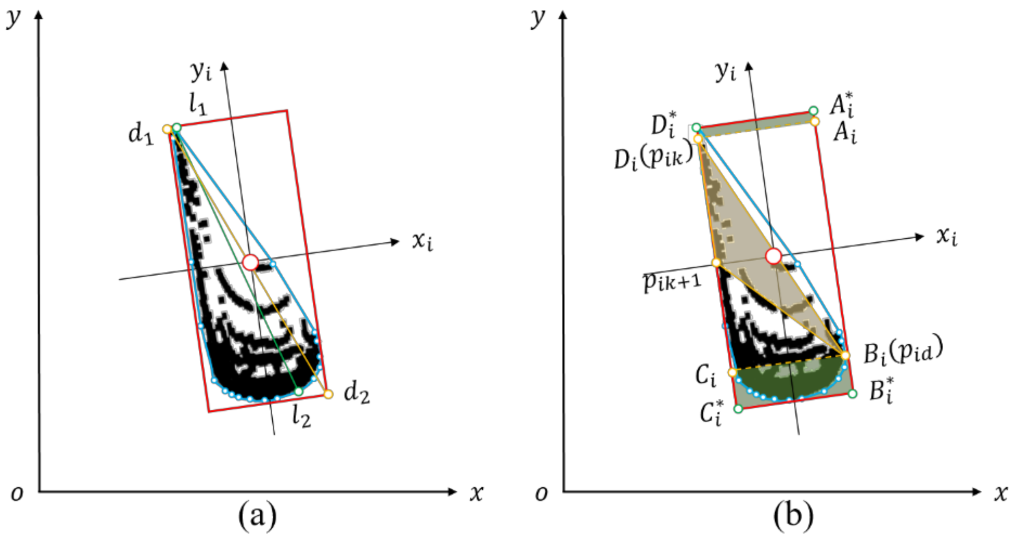
In some situations, the longest line of point clouds l 1 l 2 is not the diagonal direction d 1 d 2 , as shown in Figure 12a. Therefore, we propose the Rotating Triangle (RT) algorithm, which was explicitly designed for this situation. In the convex hull point set H , for the n convex hull points p i j contained therein, the main idea of the RT algorithm is to use any two neighbor convex hull points p i k and p i k + 1 as the base of the triangle. The vertex p i d of the triangle in the convex hull points p i j , j 1 , , k 1 , k + 2 , , n are found, and the area S i k of Δ p i k p i k + 1 p i d is calculated. When the triangle area S i k reaches the maximum, the direction of the triangle base p i k p i k + 1 is the direction of the obstacle. The height h i d of the triangle is the width of the obstacle vehicle. Each side of the convex hull forms the triangle as the base is continuously rotated in the convex hull until the largest area triangles are found. This is called the RT algorithm, an illustration of which is shown in Figure 12. Some points are not contained in the bounding box, so the Correction function is used again. It is then modified to obtain a perfect pose estimation result.

2.2.5. Comparison of Our Vehicle Pose Estimation Methods

Figure 13 shows the pose estimation results of the five proposed methods in small curvature roads and crossroads in urban areas. It can be seen that each method had its own pose estimations features.
Figure 13a,f illustrate the Basic Line algorithm’s effect. This method was found to be accurate when used on small curvature roads. However, it is not sensitive enough, especially when entering a crossroads. Figure 13f shows that the direction of the pose estimation remained north, and the pose estimation was almost entirely incorrect. Therefore, this method is only valuable for straight roads. Figure 13b,g show the RPCA algorithm’s effects. The sensitivity of the pose estimation direction was improved. Although it was not as effective as Basic Line on small curvature roads, it partly increased the sensitivity of the direction estimation. Figure 13c,h show the DPCA algorithm’s effects. The direction of some obstacles was estimated with higher accuracy. However, DPCA’s pose estimation effect was not as good as that of RPCA. Figure 13d,i show the LD algorithm’s effects; this is a more compact pose estimation method. Figure 13e,j show the effect of the RT algorithm. The global pose estimation effect of the RT algorithm was found to be the best of all methods, though it still struggled with some obstacles, such as Obj.b.
Table 1 shows the evaluation results of the above-mentioned obstacles’ (Obj.a–Obj.h) pose estimation. There is no guarantee that a perfect pose estimation result can be obtained for all obstacles if one only uses a single algorithm. However, for any obstacle vehicle, the above-discussed five methods can guarantee at least one effective pose estimation result. As such, we then needed to determine which of our methods is optimal when facing different obstacles.

2.3. Pose Estimation Evaluation Indexes

For this section, four indexes were designed to quantitatively evaluate the effects of the five pose estimation methods. The four evaluation indexes are used to estimate the bounding box pose from the time and spatial dimensions.

2.3.1. The Area of the Bounding Box

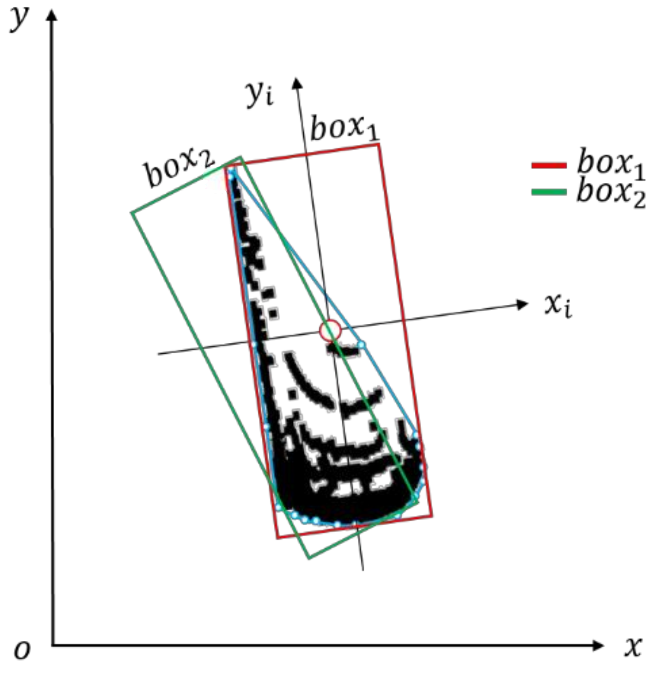
The area of the bounding box index evaluates pose estimation from the spatial dimension. Our approach was intended to allow the bounding box to more compactly enclose all point clouds of obstacles. We found that when the bounding box could enclose all point clouds, the bounding box area of its pose estimation was negatively related to its effect, as shown in Figure 14.

2.3.2. Number of Points in the Bounding Box

The minimum area discussed earlier is meaningless when the pose estimation bounding box cannot enclose all obstacle point clouds. In extreme cases, the area of the two-dimensional bounding box of the pose estimation can approach infinitesimal values. Although it approximates the smallest bounding box area, it fails to enclose any point cloud belonging to the obstacle, as shown in Figure 15.
The bounding box area at this time is no longer suitable for evaluating pose estimation results. Because of this situation, it is necessary to evaluate the number of points enclosed by the bounding box for each pose estimation. This index counts the number of point clouds in each bounding box, as shown in Figure 15.

2.3.3. The Centroid of the Bounding Box

In order to further estimate the deviation of the bounding box from the original obstacle point cloud in the spatial dimension, we established a bounding box centroid evaluation index, as shown in Figure 16.
The convex hull point set H = p i 1 , p i 2 , , p i n contains n convex hull points for the i obstacle vehicle in each frame of point cloud data H = p i 1 , p i 2 , , p i n . Firstly, it needs to calculate the distance from the point p i j to the bounding box’s four sides d j u , d j d , d j l , and d j r . Secondly, the geometric mean d j u d j d and d j l d j r of each point are calculate. The geometric mean value of the distance in the two directions is multiplied to reflect the total deviation degree in the horizontal and vertical directions. Finally, the average deviation degree of all convex hull points is calculated with Equation (11).
w i = 1 n j = 1 n d j u d j d × d j l d j r
where w i represents the average value of the deviation of all points in the horizontal and vertical directions. The smaller the centroid w i of the bounding box, the tighter the bounding box to the obstacle point cloud.

2.3.4. Direction Angle Association

These indexes must be evaluated from both the spatial and time dimensions. Sudden changes in vehicle direction are generally impossible to produce in consecutive frames. Therefore, our method associates the obstacle vehicles’ direction changes with the front and rear frames. This index can eliminate the possible fluctuation problem of direction estimation.
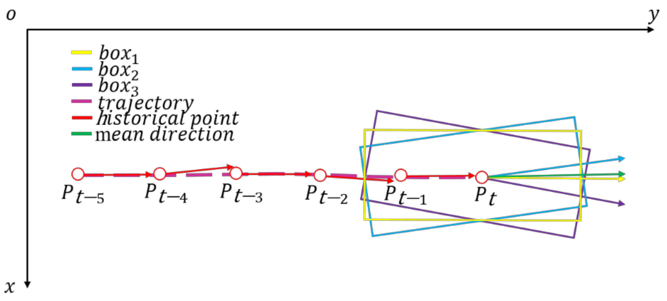
This index first uses each obstacle’s previous five frames of pose estimation direction to calculate the direction’s average value. Secondly, it calculates each pose estimation method’s direction difference between the current estimation direction and the average value of the previous five frames. That with the most minor direction difference is the best current pose estimation result, as shown in Figure 17.
The four proposed evaluation indexes quantitatively evaluate pose estimation results from the spatial and time dimensions. When evaluating the five pose estimation methods using these indexes, relying solely on one index is not a comprehensive evaluation. Therefore, four indexes need to be integrated. The relationship between the four indexes is further discussed in the next section in order to obtain the best pose estimation method.

2.4. Optimal Vehicle Pose Estimation Method Based on Ensemble Learning

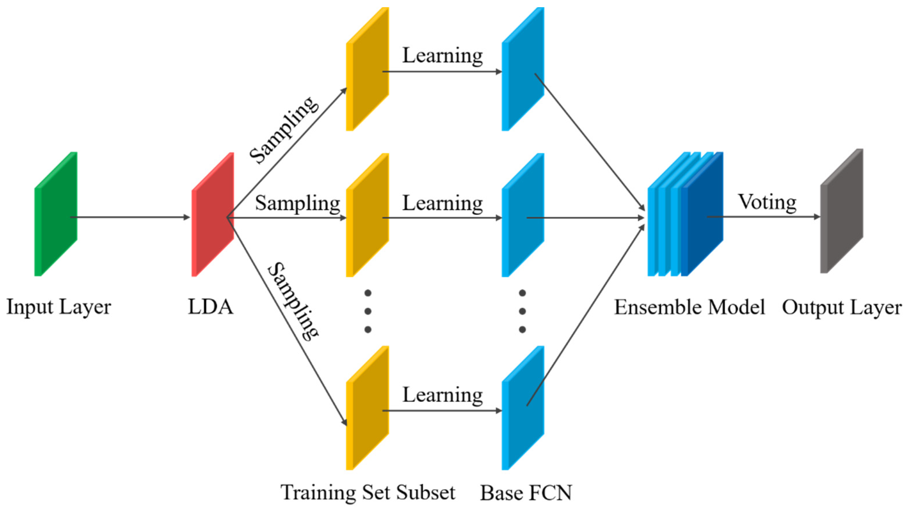
A neural network is used to compare the output with the corresponding ground truth for each input to accordingly adjust the weight. It repeats this process until the maximum number reaches the allowed iterations or an acceptable error rate is reached. This fits our requirements. The proposed network is shown in Figure 18.
The authors of this paper propose five pose estimation methods for any obstacle and four evaluation indexes for each pose estimation method. Therefore, for any obstacle, there are 20 evaluation indexes. These 20 evaluation indexes are used as the network’s input, and the ground truth is the optimal pose estimation method. This problem can be regarded as a five-classification problem with 20 feature vectors. “Optimal” refers to selecting each obstacle vehicle’s most suitable result among the proposed five pose estimation methods. Although the network may provide deviating pose estimation results, its pose estimation is relatively optimal. Our approach uses an ensemble learning algorithm based on neural networks to improve generalization. Each learner adopts a homogeneous integrated neural network architecture that uses a fully connected network. Our approach uses bootstrap sampling to construct a sub-training set of each base learner. The base learner is trained in parallel based on each sub-training set. Furthermore, the voting algorithm combines the prediction output to obtain the final prediction result.

3. Experimental Results and Discussion

3.1. The Details of TS-OVPE Network

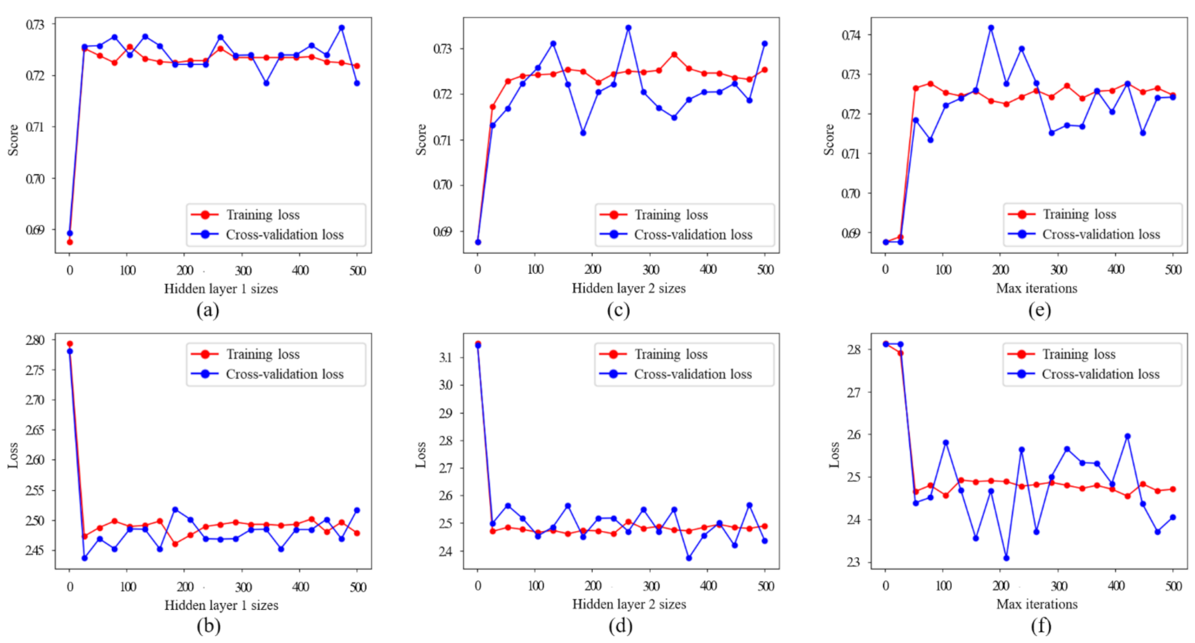
The stability of ensemble learning greatly depended on the stability of the base learner. Therefore, the parameters of the base learner first had to be determined. Because the input feature vectors of each base learner were relatively small, over-fitting was most likely to occur. The high dimensionality of the model was the primary cause of the overfitting problem. Three main hyperparameters affected this problem: the number of hidden layers, the number of neurons, and the number of iterations. The authors of this paper drew a verification curve by continuously increasing these three hyperparameters to find the optimal hyperparameter value of the base learner, as shown in Figure 19.
When the scale of the network was insufficient, the fitting ability of the base learner was too. At this time, deviation dominated the error. With the deepening of the network scale, the fitting ability of the base learner became more robust and the base learner even learned from slight fluctuations of the data. At this time, variance dominated the error. As shown in Figure 19a,b, the number of neurons in the first hidden layer of the base learner was determined to be 400, which was twenty times the number of input nodes. According to Figure 19c,d, the number of neurons in the second hidden layer of the base learner was determined to be 400. At this time, the disturbance of the model was minor. Considering the real-time requirement, we did not continually increase the number of hidden layers, and we kept the number of hidden layers to 2. According to Figure 19e,f, it was determined that the maximum number of iterations of the base learner was 200, which reduced the computational complexity of the network while ensuring its learning ability.
After determining the hyperparameters that affected the base learner’s network scale, the Relu activation function was adopted to prevent gradient disappearance caused by the saturation of the activation function. The quasi-Newton method was used in the weight optimization process. Each iteration only used gradient information, and the change between the gradients was measured to produce a super-linear convergence effect.
In the network of TS-OVPE, the number of base learners and the number of samples in the sub-training set were the essential hyperparameters that determined the effect of network learning. The number of base learners determined the degree of network fitting. If it was too small, it led to the under-fitting of the network. If it was too big, it led to network over-fitting. Thus, an appropriate number of base learners was essential. When the numbers of the base learners were 0–50, the effect of the learners was significantly improved according to our experiments. Therefore, the number of the base learners was set to 40.
The samples in the sub-training set had to be at least nearly one-third of the total samples to ensure that each sub-training set’s samples were sufficiently rich. Since the base learner was optimized, the ensemble learning performance was only improved by 10-8 when the sub-training set samples were added. Therefore, each sub-training was set at one-third of the total initial training samples while considering the algorithm’s time complexity.
Our TS-OVPE network dataset used 800 obstacle vehicles as training data from the 00 sequences of the SemanticKITTI [39] dataset. The SemanticKITTI dataset provided obstacle labels of the original point cloud, which allowed us to know which point cloud belonged to which obstacle. Our approach used the five pose algorithms to calculate its pose estimation bounding box according to each obstacle vehicle’s point cloud. Then, we calculated the four evaluation indexes of each algorithm. The network’s input comprised these twenty evaluation indexes of each obstacle vehicle. Furthermore, we annotated the optimal pose estimation algorithm’s number as the ground truth for each obstacle vehicle. The network’s training results are shown in Table 2.
These results prove that the ensemble learning could effectively improve the classification performance of the network. The ensemble learning slightly enhanced its performance because the base learner had been optimized. However, these results only reflect the performance of the proposed network; they do not reflect the effect of the pose estimation results. Methods for the evaluation of pose estimation results are discussed in Section 3.2.

3.2. Evaluation Index of Pose Estimation Results: Polygon Intersection over Union

In this section, we discuss our pose estimation evaluation index, which is used because the current dataset cannot provide rich enough information without additional manual annotations. The KITTI dataset provides raw data and annotation information for different tasks [40]. The ground truth of the clustering of each obstacle vehicle needs to be input since both our method and comparison method use each obstacle’s point cloud as the input. To accurately compare the different pose estimation algorithms, it was necessary to eliminate the interference of the inputting inaccuracy. Therefore, the authors of this paper selected the SemanticKITTI dataset with frame-by-frame annotations.
Although the input problem was solved, the SemanticKITTI dataset has mainly been proposed for the semantic segmentation of point clouds because it does not provide the bounding box’s ground truth for pose estimation. The object detection and target tracking dataset of the KITTI dataset provide the ground truth of the vehicle’s pose estimation bounding box. However, the object detection dataset comprises discrete single-frame data in which the timing information is lost, and the dataset provides the ground truth of point cloud clustering. Therefore, the authors of this paper propose a polygon intersection over union (P-IoU) evaluation standard to quantitatively measure the effect of pose estimation based on the current SemanticKITTI dataset without additional manual annotation.
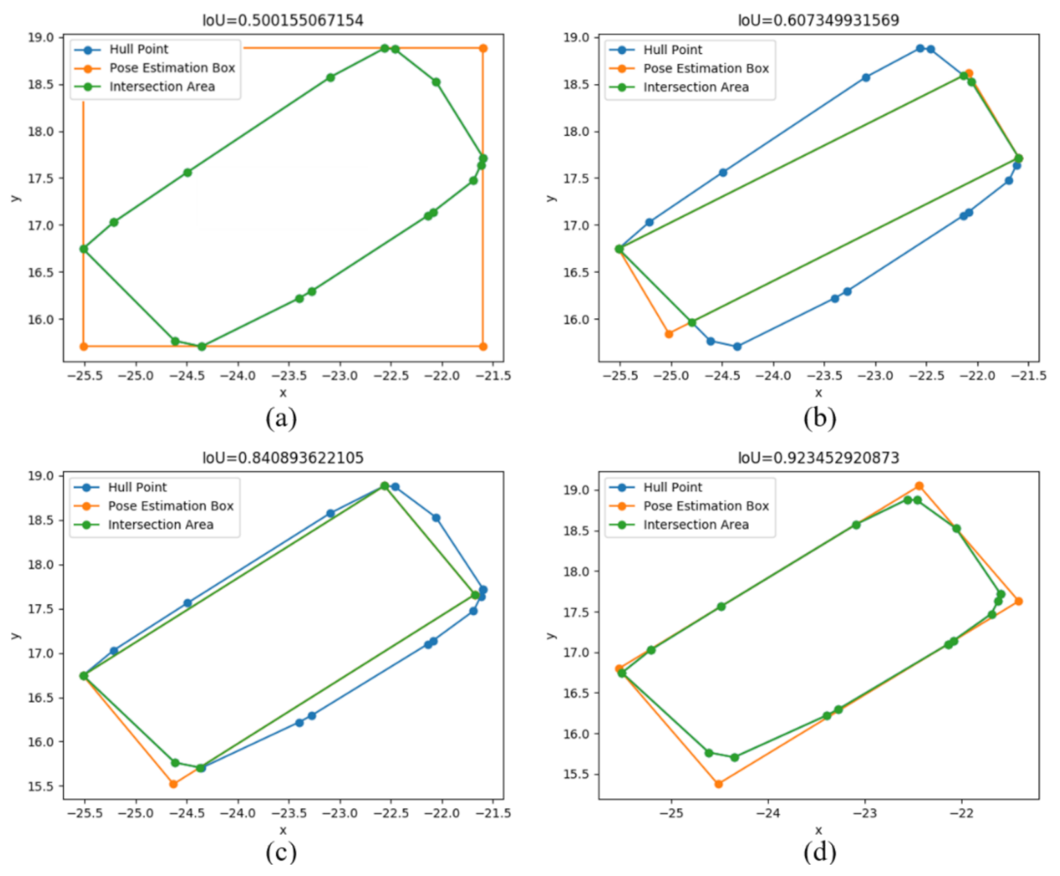
Intersection over union (IoU) is usually used to measure the overlap ratio between the candidate and ground truth bound generated in object detection. The authors of this paper used the polygon formed by the convex hull points as the original labeled box due to the lack of the bounding box’s ground truth. The two-dimensional bounding box obtained by the pose estimation algorithm was used as the candidate box to calculate the intersection ratio. The overlap ratio between them could be used to measure the effect of pose estimation, which is called P-IoU.
In an ideal situation, the P-IoU is close to 1 when its intersection and union ratio are entirely overlapped. It is worth noting that the shape of the convex hull is often not a regular rectangle, so even the bounding box could perfectly estimate the vehicle’s pose, and the P-IoU at this time is not close to 1. Because the convex hull points of different detection obstacles are different, comparing the P-IoU of different obstacles is not sensible. The P-IoU is used to compare the effect of the same obstacles of different pose estimation methods in the same frame, as shown in Figure 20.
Figure 20 verifies that our P-IoU index could effectively evaluate the pose estimation’s results. When the direction and size estimation results of the pose estimation were both inaccurate, as shown in Figure 20a, the value of P-IoU was only 50.02%. As the accuracy of the direction estimation increased, the value of P-IoU increased to 60.73%, as shown in Figure 20. However, its size estimation result still had a large error at this time. When the size estimation was closer to the obstacle vehicle’s actual size, the value of P-IoU continuously increased, as shown in Figure 20c,d. Figure 20d shows the most accurate pose estimation results obtained with the four tested indexes. Moreover, this index’s P-IoU value was also the highest at 92.25%. This set of experiments verified that the proposed P-IoU evaluation index is reasonable, and we used this index to evaluate our methods in subsequent experiments.

3.3. Experimental Results of SemanticKITTI Dataset

We texted the 00 sequences of the SemanticKITTI dataset to quantitatively evaluate the pose estimation method. The 00 sequence contains 4540 consecutive frames of LiDAR data under various road conditions in urban environments. It contains 67,085 obstacle vehicles, including 273 dynamic vehicles and 66,812 static vehicles. The dataset was divided into straight sections and curved sections via the changes of the curvature. We separately evaluated the pose estimation methods under different road sections. The distribution of obstacle vehicles under each road section is shown in Table 3.
The point cloud cluster ground truth of each obstacle vehicle marked by the SemanticKITTI dataset was used as the original input in the test. The evaluation index adopted the P-IoU proposed in the previous section. According to the road differentiation conditions in Table 3, tests were carried out on straight and curved roads. The authors of this paper compared the L-shaped pose estimation method [31] and the global pose estimation method [17], they are the latest two mainstream pose estimation methods. Table 4 shows the results of the comparative experiment.
As shown in Table 4, our approach was superior to the two comparison methods on any road section. The two compared methods had poor performance on the curved road sections. Our approach was found to have advantages on curved road sections. Our method had this apparent advantage because of the proposed direction angle association evaluation index. The methods of [31] and [17] cannot be corrected when a direction estimation error occurs since it is estimated in a single frame. Our method considers the direction of the first few frames to improve the accuracy of pose estimation. Our approach was found to be very stable on all road sections and remained at almost the same level. The fluctuation range of the P-IoU was within 0.25%. The accuracy of P-IoU was significantly improved by 5.25% and 9.67% in comparison to the two methods.
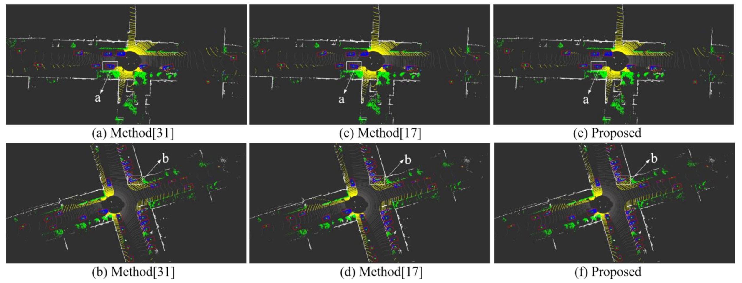
Figure 21 shows the experimental results of one frame for each of the two road conditions. These results were consistent with the results of the P-IoU. Obviously, the accuracy of the method of [17] was less effective than that of [31], especially for the curved road sections. Although the method of [31] was much better than the method of [17] at direction estimation, it sometimes also had estimation errors, as shown in Figure 21b. Our method showed a good pose estimation robustness on both straight and curved road sections all the time.
Figure 22 shows the P-IoU evaluation. The two compared methods substantially correctly estimate the obstacle’s direction, but its direction and size are not compact enough, as shown in Figure 22a. In Figure 22b, the direct estimation of Method [31] is obviously wrong, and the size of the pose estimation of Method [17] is not compact enough. Although Method [31] has better overall performance than Method [17], its stability is not as good as ours.

3.4. Experimental Results of Our Experimental Platform

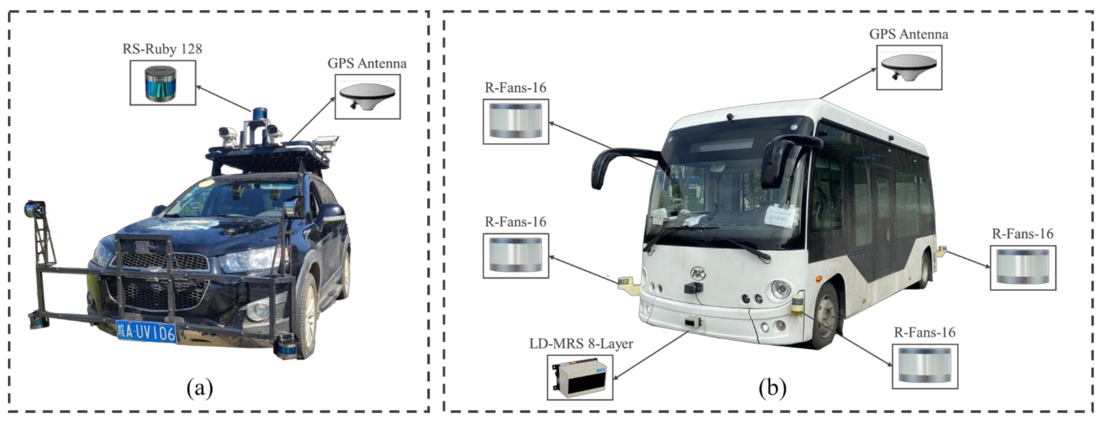
To test our approach’s effect in the actual road environment, this paper tests on our "Smart Pioneer" experimental platform. The specific layout plan of the "Smart Pioneer" experimental platform is shown in Figure 23. We do not choose the same 64-line LiDAR as the SemanticKITTI dataset but used 128-line LiDAR on the "Smart Pioneer" experimental platform to verify the generalization performance of our approach. The parameters of the "Smart Pioneer" experimental platform as shown in Table 5.
When only one vehicle is used for the experiment, the actual pose of the obstacle vehicles cannot be obtained. Therefore, our approach configured the two experimental vehicles. Since both vehicles are equipped with GPS receiving equipment, the GPS receiving equipment can provide the ground truth of the vehicle pose in real time.
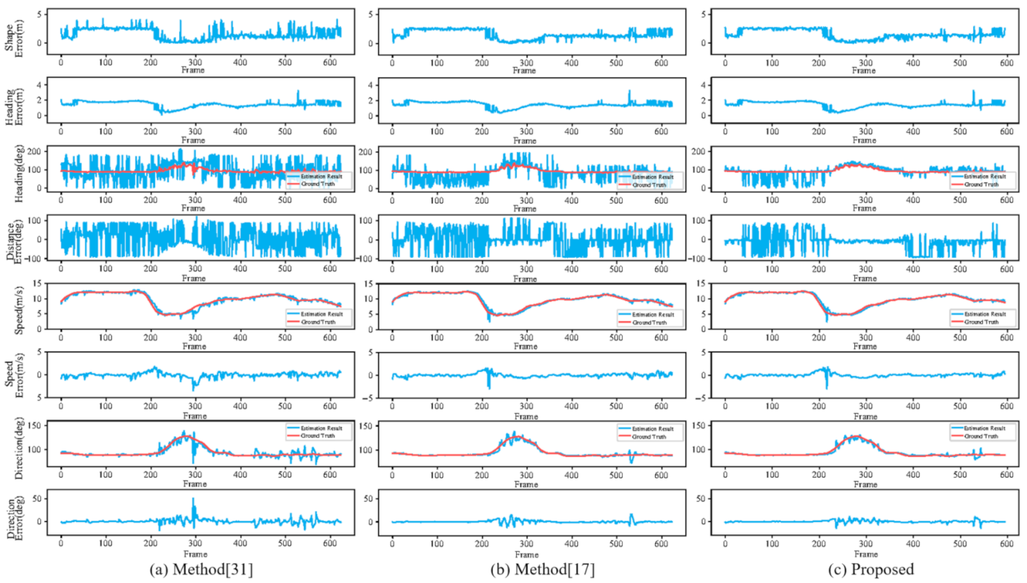
This paper verifies the accuracy of the pose estimation algorithm itself and its effect on the object tracking algorithm. The experiment details are as follows: the "Smart Pioneer" SUV platform is used as the experimental vehicle, and the "Smart Pioneer" Minibus platform is used as the target obstacle vehicle. The two vehicles are tested in a regular urban environment, and the vehicle’s trajectory is designed to be on a right turn road section. This paper uses ground segmentation with the original point cloud [15] and then performs clustering processing [16] in the process of point cloud data. Moreover, we use the object tracking algorithm [41] to evaluate the pose estimation algorithm’s effect on tracking results. The experimental results are shown in Figure 24.
Compared with the two methods of comparison, our approach has certain advantages in pose estimation. Table 6 shows the evaluation indexes related to the pose estimation. Our approach has the smallest mean error on various road sections. The standard deviation of the error is also relatively low, which means our approach has stable performance. Our approach has a significant advantage in heading estimation. The experimental results are consistent with the performance on the public SemanticKITTI dataset. The average error of our approach is reduced 11.87 degrees and 22.40 degrees smaller than Method [31] and Method [17] in the global heading estimation. The average heading error reduces by about 29.49% and 44.11% on all road sections. The advantage of heading estimation is more obvious on the curved roads sections, and the mean value of the heading estimation error is reduced 21.64 degrees and 33.85 degrees than Method [31] and Method [17].
The mean value of the heading error is higher than the standard deviation of the heading error, which indicates that the heading results have a high dispersion degree. Two reasons cause this volatility: (1) The partial lack of the original point cloud cannot truly reflect the shape of the obstacle. (2) In preprocessing, the inaccurate clustering will cause the same obstacle to be clustered into two objects or combine obstacles into one object. These two situations randomly occur, which has a significant influence on heading estimation. Since the heading estimation is calculated based on the input point cloud, the inaccurate input will indirectly make pose estimation results showing a huge heading error. The experiment uses the same input and evaluation methods, and it can be seen that our method reduces this dispersion of heading estimation as much as possible.
The shape and position estimation results of the three methods are almost identical, as shown in Figure 24. Our method only slightly improves the performance because these two parameters depend on the original point cloud. The algorithm can only get the shape from the original incomplete point cloud, as shown in Figure 25. The fundamental shape error is the same, and it is not easy to restore the complete point cloud. The distance estimation is calculated using the center point of the obstacle vehicle’s bounding box. The position is similar because its shape estimation has already received the same limitation from the point cloud. In our experiment, although the standard deviation of some indexes is not as good as the compared methods, our approach always has a lower error. Our approach achieves the best accuracy while ensuring the stability of the algorithm.
In the experiment of object tracking, our approach also has apparent advantages. As shown in Table 6, our approach has obvious advantages in the speed direction evaluation of the tracking algorithm. Compared with Method [31] and Method [17], the error of speed direction is reduced by 0.06 degrees and 1.33 degrees. The average speed direction error reduces by about 3.85% and 46.70%. The speed error is caused by the accumulation of position error, which will amplify the position error. As shown in Table 6, our position estimation has only a slight advantage, but this advantage is magnified in speed estimation. Compared with Method [17], our position error is only reduced by 0.02 meters on the curved roads, but its speed error is reduced by 0.2 m/s. Although our approach only has a slight increase in the object tracking’s speed estimation, this slight improvement is also essential considering the high moving speed of object vehicles.

4. Discussion

Our experiments proved our method has accurate pose estimation results. The pose estimation methods usually only use a single pose estimation method [17,31]. Due to the diversity of point cloud distribution, it is hard to get perfect pose estimation results for all obstacle vehicles. As shown in Figure 21, Method [31] and Method [17] are not stable on both straight and curved road sections. We used the TS-OVPE network to determine each obstacle’s best pose estimation methods from one of the five proposed methods. The five proposed pose estimation methods complemented each other and ensured that each obstacle had a perfect pose estimation result, as shown in Table 1. Compared with other methods [17,31], our approach used the road direction, which was usually ignored as a priori pose estimation. This method efficiently estimated pose on the straight road, as shown in Figure 13a. Unlike the method of [38], we did not directly use PCA; instead, we used the RPCA and DPCA algorithms combined with the distribution feature of the point cloud, as shown in Figure 7. These two algorithms used PCA results as an a priori direction to improve the pose estimation performance on curved road sections, as shown in Figure 13g,h. Due to the complex environment of actual roads, the severe lack of point cloud data makes pose estimation difficult. Thus, we used the LD and RT algorithms to fix this problem with better global adaptability, as shown in Figure 13i,j. The proposed evaluation indexes considering the time and spatial dimensions converted the five pose estimation methods into a unified dimension for training. Most pose estimation algorithms are processed in a single frame, but our direction angle association index made the method more robust than other methods. As shown in Figure 24c, the heading curve of our method was closer to the ground truth and possessed more minor fluctuation than the other methods. As shown in Figure 22, the combined effect of multiple spatial evaluation indexes enhanced our pose estimation. As we mentioned in the introduction, poor generalization is the biggest problem of neural networks. Therefore, we indirectly trained the TS-OVPE network through the proposed evaluation indexes. The network was trained on the public SemanticKITTI dataset, which used 64-line LiDAR. As shown in Table 6, it unexpectedly maintained a good pose estimation performance on our own dataset. In summary, our TS-OVPE network is able to effectively improve the accuracy of pose estimation. Moreover, it has a sensitive direction estimation feature and also shows excellent performance on curved road sections.
Although our method can obtain effective pose estimation results in most cases, it still has the following limitations. (1) Due to the lack of the original point cloud, it makes the size estimation of vehicle obstacles more difficult. The incompleteness of the obstacle’s point cloud greatly restricts the pose estimation algorithms. (2) Our method relies on the distribution density of the point cloud. Its good adaptability has been verified for multi-line LiDAR. However, the point cloud density in low-line LiDAR is too sparse to enable effective pose estimation results.
In the future, we will continue to improve pose estimation accuracy in two respects. (1) We will research pose estimation algorithms based on camera–LiDAR fusion because this fusion could obtain richer obstacle information [42]. The sole use of point cloud makes it challenging to identify obstacle types. However, it is easier to detect obstacle types from camera images. The obstacle type, such as car, truck, and bus, can be merged with the point cloud clustering results. The template matching method can be used to fill the missing part of the obstacle point cloud. With the whole shape of the point cloud, the pose estimation can be made more accurate and reliable. Moreover, it also makes pose estimation under low-line LiDAR possible. (2) Inertial measurement unit (IMU) sensors can be used to obtain a vehicle’s motion state in the pose estimation processing. IMU sensors can provide a vehicle’s kinematics and dynamics parameters, such as angular velocity and acceleration [43,44]. These parameters can help obtain a vehicle’s driving states, such as on a straight road section or a curved road section. More abundant prior information can make pose estimation more accurate.

5. Conclusions

The authors of this paper have proposed an optimal vehicle pose estimation network based on time series and spatial tightness with 3D LiDAR. The network integrates five pose estimation algorithms to face changeable point cloud distributions. It eliminates dependence on the specific point cloud’s geometric shape, such as the most commonly used feature: L-shape. Under the ensemble learning unit, our network can effectively achieve optimal pose estimation that is stable for both static and dynamic obstacle vehicles. In the SemanticKITTI dataset, compared with the other two methods, the P-IoU was found to improve by 5.25% and 9.67%, which showed its accuracy when there was no interference from preprocessing. This performance depended on the time and spatial evaluation indexes during network training. With the combination of time series and spatial tightness, our network showed a stable pose estimation performance on all roads sections. It even maintained the same level on curved road sections, which was the hardest for the other pose estimation algorithms. On the SemanticKITTI dataset, the fluctuation range of our algorithm’s P-IoU was only within 0.25%. Since the evaluation index of each method is used for indirect training, our network can be directly used on our platform even if the LiDAR-line is entirely different. The actual urban road experiment showed that our pose estimation algorithm had an accurate heading estimation. The average heading error was reduced by about 29.49% and 44.11% on all road sections due to the integration of PCA methods into our algorithm. To test whether the application of the proposed pose estimation algorithm was practical, we also tested its effect on an object tracking algorithm. The object tracking results showed that our algorithm could reduce the average speed direction error by about 3.85% and 46.70% compared with the two methods. In conclusion, our algorithm not only improves pose estimation’s adaptability and direction sensitivity but also has practical application value for tracking algorithms.

Author Contributions

Conceptualization, H.W., Z.W. and L.L.; methodology, H.W. and F.X.; formal analysis, H.W. and F.X.; data curation, H.W. and J.Y.; writing—original draft preparation, H.W.; writing—review and editing, Z.W., L.L. and H.L.; visualization, H.W. and J.Y.; supervision, Z.W.; funding acquisition, H.L. All authors have read and agreed to the published version of the manuscript.

Funding

This work was supported by the Key Supported Project in the Thirteenth Five-Year Plan of Hefei Institutes of Physical Science, Chinese Academy of Sciences (Grant No. KP-2019-16), Natural Science Foundation of Anhui Province (Grant No. 1808085QF213), Key Science and Technology Project of Anhui (Grant No. 202103a05020007), and Technological Innovation Project for New Energy and Intelligent Networked Automobile Industry of Anhui Province.

Institutional Review Board Statement

Not applicable.

Informed Consent Statement

Not applicable.

Data Availability Statement

A publicly available dataset was analyzed in this study. The data can be found here: http://www.semantic-kitti.org/ (accessed on 17 August 2021). Some data presented in this study are available on request from the corresponding author. The data are not publicly available due to the confidentiality clause of some projects.

Conflicts of Interest

The authors declare no conflict of interest.

Abbreviations

The following abbreviations are used in this manuscript.
AVAutonomous Vehicle
LiDARLight Detection and Ranging
TS-OVPEOptimal Vehicle Pose Estimation Based on Time Series and Spatial Tightness
PCAPrincipal Component Analysis
RPCARotating Principal Component Analysis
DPCADiagonal Principal Component Analysis
LDLongest Diameter
RTRotating Triangle
IoUIntersection over Union
P-IoUPolygon Intersection over Union
ROSRobot Operating System
IMUInertial Measurement Unit

References

  1. Khatab, E.; Onsy, A.; Varley, M.; Abouelfarag, A. Vulnerable objects detection for autonomous driving: A review. Integration 2021, 78, 36–48. [Google Scholar] [CrossRef]
  2. Su, Z.; Hui, Y.; Luan, T.H.; Liu, Q.; Xing, R. Deep Learning Based Autonomous Driving in Vehicular Networks. In The Next Generation Vehicular Networks, Modeling, Algorithm and Applications, 1st ed.; Springer: Cham, Switzerland, 2020; pp. 131–150. [Google Scholar] [CrossRef]
  3. Du, X.; Ang, M.H.; Karaman, S.; Rus, D. A general pipeline for 3d detection of vehicles. In Proceedings of the IEEE International Conference on Robotics and Automation (ICRA), Brisbane, Australia, 21–25 May 2018; pp. 3194–3200. [Google Scholar] [CrossRef] [Green Version]
  4. Du, L.; Ye, X.; Tan, X.; Feng, J.; Xu, Z.; Ding, E.; Wen, S. Associate-3Ddet: Perceptual-to-Conceptual Association for 3D Point Cloud Object Detection. In Proceedings of the IEEE/CVF Conference on Computer Vision and Pattern Recognition (CVPR), Seattle, WA, USA, 13–19 June 2020; pp. 13326–13335. [Google Scholar] [CrossRef]
  5. Tan, M.; Pang, R.; Le, Q.V. EfficientDet: Scalable and Efficient Object Detection. In Proceedings of the IEEE/CVF Conference on Computer Vision and Pattern Recognition (CVPR), Seattle, WA, USA, 13–19 June 2020; pp. 10778–10787. [Google Scholar] [CrossRef]
  6. Bochkovskiy, A.; Wang, C.-Y.; Liao, H.-Y.M. YOLOv4: Optimal Speed and Accuracy of Object Detection. arXiv 2020, arXiv:2004.10934. [Google Scholar]
  7. Wang, T.; Anwer, R.M.; Cholakkal, H.; Khan, F.S.; Pang, Y.; Shao, L. Learning rich features at high-speed for single-shot object detection. In Proceedings of the IEEE/CVF International Conference on Computer Vision (ICCV), Seoul, Korea, 27–28 October 2019; pp. 1971–1980. [Google Scholar] [CrossRef]
  8. Liu, S.; Huang, D. Receptive field block net for accurate and fast object detection. In Proceedings of the European Conference on Computer Vision (ECCV), Munich, Germany, 8–14 September 2018; pp. 385–400. [Google Scholar] [CrossRef] [Green Version]
  9. Ren, S.; He, K.; Girshick, R.; Sun, J. Faster R-CNN: Towards Real-Time Object Detection with Region Proposal Networks. IEEE Trans. Pattern Anal. Mach. Intell. 2017, 39, 1137–1149. [Google Scholar] [CrossRef] [Green Version]
  10. Shi, S.; Guo, C.; Jiang, L.; Wang, Z.; Shi, J.; Wang, X.; Li, H. PV-RCNN: Point-Voxel Feature Set Abstraction for 3D Object Detection. In Proceedings of the IEEE/CVF Conference on Computer Vision and Pattern Recognition (CVPR), Seattle, WA, USA, 13–19 June 2020; pp. 10526–10535. [Google Scholar] [CrossRef]
  11. Zhou, J.; Tan, X.; Shao, Z.; Ma, L. FVNet: 3D Front-View Proposal Generation for Real-Time Object Detection from Point Clouds. In Proceedings of the 12th International Congress on Image and Signal Processing, BioMedical Engineering and Informatics (CISP-BMEI), Kunshan, China, 19–21 October 2019; pp. 1–8. [Google Scholar] [CrossRef] [Green Version]
  12. Beltrán, J.; Guindel, C.; Moreno, F.M.; Cruzado, D.; García, F.; Escalera, A.D.L. BirdNet: A 3D Object Detection Framework from LiDAR Information. In Proceedings of the 21st International Conference on Intelligent Transportation Systems (ITSC), Maui, HI, USA, 4–7 November 2018; pp. 3517–3523. [Google Scholar] [CrossRef] [Green Version]
  13. Geiger, A.; Lenz, P.; Stiller, C.; Urtasun, R. Vision meets robotics: The KITTI dataset. Int. J. Robot. Res. 2013, 32, 1231–1237. [Google Scholar] [CrossRef] [Green Version]
  14. Wu, Y.; Wang, Y.; Zhang, S.; Ogai, H. Deep 3D Object Detection Networks Using LiDAR Data: A Review. IEEE Sensors J. 2021, 21, 1152–1171. [Google Scholar] [CrossRef]
  15. Huang, W.; Liang, H.; Lin, L.; Wang, Z.; Wang, S.; Yu, B.; Niu, R. A Fast Point Cloud Ground Segmentation Approach Based on Coarse-To-Fine Markov Random Field. IEEE Trans. Intell. Transp. Syst. 2021. Early Access. [Google Scholar] [CrossRef]
  16. Yang, H.; Wang, Z.; Lin, L.; Liang, H.; Huang, W.; Xu, F. Two-Layer-Graph Clustering for Real-Time 3D LiDAR Point Cloud Segmentation. Appl. Sci. 2020, 10, 8534. [Google Scholar] [CrossRef]
  17. Yang, J.; Zeng, G.; Wang, W.; Zuo, Y.; Yang, B.; Zhang, Y. Vehicle Pose Estimation Based on Edge Distance Using Lidar Point Clouds (Poster). In Proceedings of the 22th International Conference on Information Fusion (FUSION), Ottawa, ON, Canada, 2–5 July 2019; pp. 1–6. [Google Scholar]
  18. An, J.; Kim, E. Novel Vehicle Bounding Box Tracking Using a Low-End 3D Laser Scanner. IEEE Trans. Intell. Transp. Syst. 2021, 22, 3403–3419. [Google Scholar] [CrossRef]
  19. Li, Y.; Ibanez-Guzman, J. Lidar for Autonomous Driving: The Principles, Challenges, and Trends for Automotive Lidar and Perception Systems. IEEE Signal Process. Mag. 2020, 37, 50–61. [Google Scholar] [CrossRef]
  20. Li, Y.; Ma, L.; Zhong, Z.; Liu, F.; Chapman, M.A.; Cao, D.; Li, J. Deep Learning for LiDAR Point Clouds in Autonomous Driving: A Review. IEEE Trans. Neural Networks Learn. Syst. 2021, 32, 3412–3432. [Google Scholar] [CrossRef]
  21. Wen, C.; Sun, X.; Li, J.; Wang, C.; Guo, Y.; Habib, A. A deep learning framework for road marking extraction, classification and completion from mobile laser scanning point clouds. ISPRS J. Photogramm. Remote. Sens. 2019, 147, 178–192. [Google Scholar] [CrossRef]
  22. Kumar, B.; Pandey, G.; Lohani, B.; Misra, S.C. A multi-faceted CNN architecture for automatic classification of mobile LiDAR data and an algorithm to reproduce point cloud samples for enhanced training. ISPRS J. Photogramm. Remote. Sens. 2019, 147, 80–89. [Google Scholar] [CrossRef]
  23. Xu, F.; Liang, H.; Wang, Z.; Lin, L.; Chu, Z. A Real-Time Vehicle Detection Algorithm Based on Sparse Point Clouds and Dempster-Shafer Fusion Theory. In Proceedings of the IEEE International Conference on Information and Automation (ICIA), Wuyi Mountain, China, 11–13 August 2018; pp. 597–602. [Google Scholar] [CrossRef]
  24. Wittmann, D.; Chucholowski, F.; Lienkamp, M. Improving lidar data evaluation for object detection and tracking using a priori knowledge and sensorfusion. In Proceedings of the 11th International Conference on Informatics in Control, Automation and Robotics (ICINCO), Vienna, Austria, 1–3 September 2014; pp. 794–801. [Google Scholar] [CrossRef]
  25. Zhao, C.; Fu, C.; Dolan, J.M.; Wang, J. L-Shape Fitting-based Vehicle Pose Estimation and Tracking Using 3D-LiDAR. IEEE Trans. Intell. Veh. 2021. Early Access. [Google Scholar] [CrossRef]
  26. MacLachlan, R.; Mertz, C. Tracking of Moving Objects from a Moving Vehicle Using a Scanning Laser Rangefinder. In Proceedings of the 2006 IEEE Intelligent Transportation Systems Conference (ITSC), Toronto, ON, Canada, 17–20 September 2006; pp. 301–306. [Google Scholar] [CrossRef] [Green Version]
  27. Shen, X.; Pendleton, S.; Ang, M.H. Efficient L-shape fitting of laser scanner data for vehicle pose estimation. In Proceedings of the 2015 IEEE 7th International Conference on Cybernetics and Intelligent Systems (CIS) and IEEE Conference on Robotics, Automation and Mechatronics (RAM), Angkor Wat, Cambodia, 15–17 July 2015; pp. 173–178. [Google Scholar] [CrossRef]
  28. Wang, Z.; Wu, Y.; Niu, Q. Multi-Sensor Fusion in Automated Driving: A Survey. IEEE Access 2019, 8, 2847–2868. [Google Scholar] [CrossRef]
  29. Wu, T.; Hu, J.; Ye, L.; Ding, K. A Pedestrian Detection Algorithm Based on Score Fusion for Multi-LiDAR Systems. Sensors 2021, 21, 1159. [Google Scholar] [CrossRef]
  30. Zhang, X.; Xu, W.; Dong, C.; Dolan, J.M. Efficient L-shape fitting for vehicle detection using laser scanners. In Proceedings of the 2017 IEEE Intelligent Vehicles Symposium (IV), Redondo Beach, CA, USA, 11–14 June 2017; pp. 54–59. [Google Scholar] [CrossRef]
  31. Qu, S.; Chen, G.; Ye, C.; Lu, F.; Wang, F.; Xu, Z.; Gel, Y. An Efficient L-Shape Fitting Method for Vehicle Pose Detection with 2D LiDAR. In Proceedings of the IEEE International Conference on Robotics and Biomimetics (ROBIO), Kuala Lumpur, Malaysia, 12–15 December 2018; pp. 1159–1164. [Google Scholar] [CrossRef] [Green Version]
  32. Kim, D.; Jo, K.; Lee, M.; Sunwoo, M. L-Shape Model Switching-Based Precise Motion Tracking of Moving Vehicles Using Laser Scanners. IEEE Trans. Intell. Transp. Syst. 2017, 19, 598–612. [Google Scholar] [CrossRef]
  33. Chen, T.; Wang, R.; Dai, B.; Liu, D.; Song, J. Likelihood-Field-Model-Based Dynamic Vehicle Detection and Tracking for Self-Driving. IEEE Trans. Intell. Transp. Syst. 2016, 17, 3142–3158. [Google Scholar] [CrossRef]
  34. Chen, T.; Dai, B.; Liu, D.; Fu, H.; Song, J.; Wei, C. Likelihood-Field-Model-Based Vehicle Pose Estimation with Velodyne. In Proceedings of the 2015 IEEE 18th International Conference on Intelligent Transportation Systems (ITSC), Gran Canaria, Spain, 15–18 September 2015; pp. 296–302. [Google Scholar] [CrossRef]
  35. Naujoks, B.; Wuensche, H. An Orientation Corrected Bounding Box Fit Based on the Convex Hull under Real Time Constraints. In Proceedings of the 2018 IEEE Intelligent Vehicles Symposium (IV), Changshu, China, 26–30 June 2018; pp. 1–6. [Google Scholar] [CrossRef]
  36. Liu, K.; Wang, W.; Tharmarasa, R.; Wang, J. Dynamic Vehicle Detection with Sparse Point Clouds Based on PE-CPD. IEEE Trans. Intell. Transp. Syst. 2019, 20, 1964–1977. [Google Scholar] [CrossRef]
  37. Sklansky, J. Finding the convex hull of a simple polygon. Pattern Recognit. Lett. 1982, 1, 79–83. [Google Scholar] [CrossRef]
  38. Zhao, H.; Zhang, Q.; Chiba, M.; Shibasaki, R.; Cui, J.; Zha, H. Moving object classification using horizontal laser scan data. In Proceedings of the IEEE International Conference on Robotics and Automation (ICRA), Kobe, Japan, 12–17 May 2009; pp. 2424–2430. [Google Scholar] [CrossRef]
  39. Behley, J.; Garbade, M.; Milioto, A.; Quenzel, J.; Behnke, S.; Stachniss, C.; Gall, J. Semantickitti: A dataset for semantic scene understanding of lidar sequences. In Proceedings of the IEEE/CVF International Conference on Computer Vision (ICCV), Seoul, Korea, 27–28 October 2019; pp. 9297–9307. [Google Scholar] [CrossRef] [Green Version]
  40. Geiger, A.; Lenz, P.; Urtasun, R. Are we ready for autonomous driving? The KITTI vision benchmark suite. In Proceedings of the 2012 IEEE Conference on Computer Vision and Pattern Recognition (CVPR), Providence, RI, USA, 16–21 June 2012; pp. 3354–3361. [Google Scholar] [CrossRef]
  41. Arya, A. 3D-LIDAR Multi Object Tracking for Autonomous Driving: Multi-target Detection and Tracking under Urban Road Uncertainties. Master’s Thesis, Delft University of Technology, Delft, The Netherlands, 2017. [Google Scholar]
  42. Lee, H.; Chae, H.; Yi, K. A Geometric Model based 2D LiDAR/Radar Sensor Fusion for Tracking Surrounding Vehicles. IFAC-PapersOnLine 2019, 52, 130–135. [Google Scholar] [CrossRef]
  43. Glowinski, S.; Krzyzynski, T.; Bryndal, A.; Maciejewski, I. A Kinematic Model of a Humanoid Lower Limb Exoskeleton with Hydraulic Actuators. Sensors 2020, 20, 6116. [Google Scholar] [CrossRef] [PubMed]
  44. Slowak, P.; Kaniewski, P. Stratified Particle Filter Monocular SLAM. Remote. Sens. 2021, 13, 3233. [Google Scholar] [CrossRef]
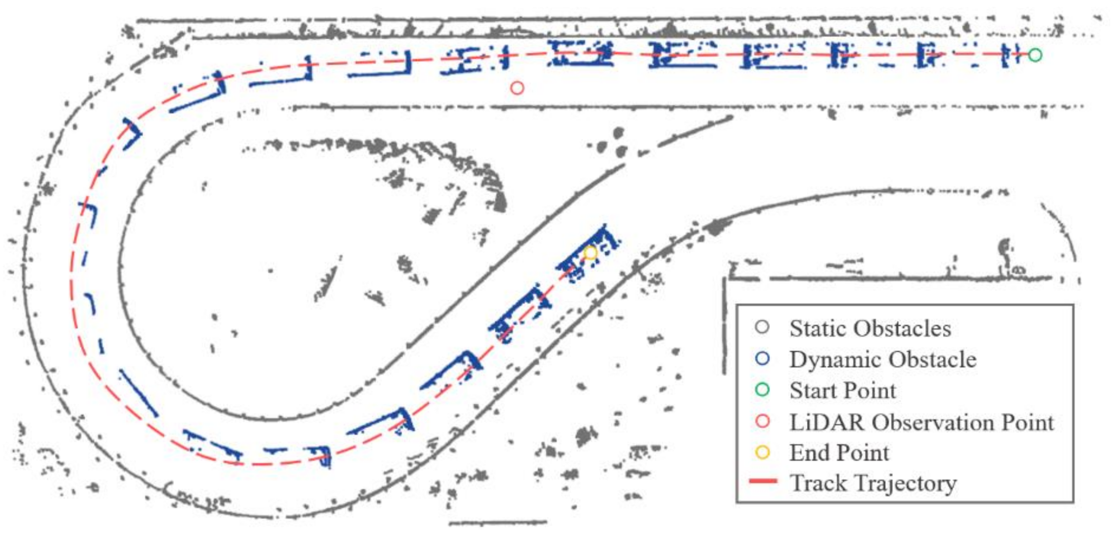
Figure 1. Point cloud scanning results of the same dynamic obstacle. When the obstacle vehicle gradually approaches our LiDAR observation point, the obstacle vehicle’s point cloud becomes dense. Otherwise, the point cloud becomes sparse. The obstacle vehicle shows L-shape, I-shape, C-shape, and other forms during this process. The variability of the point cloud’s distribution makes pose estimation challenging.
Remotesensing 13 04123 g001
Figure 2. Vehicle pose estimation result based on the 3D point cloud. The blue points represent static obstacle vehicles, the orange points represent dynamic obstacle vehicles, and the red bounding box represents the pose estimation result. Our approach can accurately estimate the tiny angular deviation of obstacle vehicles. As shown from the bird’s eye view, our approach could effectively estimate the direction of these two dynamic obstacle vehicles even if their directions only changed slightly.
Remotesensing 13 04123 g002
Figure 3. Overall flow chart. In Section 2.1, the preprocessing method is proposed. Section 2.2 presents five different pose estimation methods. Section 2.3 presents four indexes for evaluating pose estimation methods from the time and spatial dimensions. In Section 2.4, the TS-OVPE network is proposed, and introduces the network’s structure is introduced. Section 3 presents tests of the proposed algorithm in a public dataset and our experimental dataset.
Remotesensing 13 04123 g003
Figure 4. Visual representation of the vehicle pose estimation coordinate system.
Remotesensing 13 04123 g004
Figure 5. Convex hull extraction of obstacle vehicle point cloud: (a) the original 3D point cloud of the obstacle vehicle; (b) the bird’s eye view of the obstacle vehicle point cloud; (c) the convex hull point of the obstacle vehicle (red line).
Remotesensing 13 04123 g005
Figure 6. Illustration of the Basic Line algorithm. The black points represent the projection points of the original point cloud on the horizontal plane, the blue points represent the convex hull points, the blue lines represent the contour lines of the point cloud, and the yellow points represent the poles of the convex hull points in the x and y directions. The green points represent the corner point of the two-dimensional bounding box, and the red lines represent the extracted two-dimensional bounding box.
Remotesensing 13 04123 g006
Figure 7. Schematic diagram of the PCA method for extracting the driving direction of the obstacle point cloud: (a) the direction obtained by the PCA is the driving direction; (b) the direction obtained by the PCA is the diagonal direction; (c) the direction obtained by the PCA is neither the driving direction nor the diagonal direction. The red arrow represents the direction obtained by PCA.
Remotesensing 13 04123 g007
Figure 8. Illustration of the RPCA algorithm: (a) the original coordinate system of the RPCA; (b) the coordinate system after forwarding rotation. The red arrow represents the direction of obstacles extracted by the PCA. The essence of the RPCA algorithm is its use of the direction obtained by the PCA to find the corner points of the two-dimensional bounding box by twice rotating the coordinate points forward and backward.
Remotesensing 13 04123 g008
Figure 9. Illustration of diagonal obstacle point cloud formation. When the LiDAR transmitter emits a laser pulse, the emitted laser beam irradiates the surface of the obstacle object and forms the return light. Therefore, the point cloud has a diagonal shape when the obstacle vehicle’s relative position is diagonal.
Remotesensing 13 04123 g009
Figure 10. Illustration of the DPCA algorithm. The red dotted line represents the uncorrected bounding box, the red line box represents the final bounding box, and the green part represents the corrected area.
Remotesensing 13 04123 g010
Figure 11. Illustration of the LD algorithm. (a) and (d) show the left diagonal, and (b) and (c) show the right diagonal. (a) and (c) show the farthest points on the left side of the diagonal, and (b) and (d) show the farthest points on the right side of the diagonal.
Remotesensing 13 04123 g011
Figure 12. Illustration of the RT algorithm: (a) illustration of the situation faced by the RT algorithm. The longest line (green line) is not the diagonal direction (yellow line); (b) illustration of the RT algorithm. The yellow triangle represents the triangle with the largest area found by the RT algorithm, and the green part represents the corrected area. The mark "*" represents the corrected bounding box’s corner points.
Remotesensing 13 04123 g012
Figure 13. Comparison of the results of our five pose estimation algorithms. The blue point represents the obstacle vehicle point cloud, and the red box represents the bounding box of the obstacle’s pose estimation. The experimental conditions of (ae) were small curvature roads, and the experimental conditions of (fj) were crossroads.
Remotesensing 13 04123 g013
Figure 14. Illustration of the bounding box area evaluation index: (a) three different pose estimation bounding boxes; (b) a comparison of three bounding box areas. The area of box1 is the smallest, and the pose estimation of the two-dimensional bounding box is the most compact, which means its pose estimation result was the most accurate.
Remotesensing 13 04123 g014
Figure 15. Illustration of the number of points in the bounding box evaluation index. Although box2 box2 has the smallest area, its bounding box fails to enclose all the point clouds. The box2 has a larger area than box1, but it can enclose all point clouds, so box2’s pose estimation effect was better than box1.
Remotesensing 13 04123 g015
Figure 16. Illustration of the bounding box centroid evaluation index.
Remotesensing 13 04123 g016
Figure 17. Illustration of direction angle association evaluation index. P t represents the current moment, P t 1 P t 5 represent the historical trajectory points of this obstacle in the previous five frames, and the direction of the green arrow represents the average direction of the previous five frames. At the P t moment, the bounding boxes of the three pose estimation methods are shown. According to the direction angle association index, the pose estimation direction of b o x 1 is the closest to the historical average direction. Thus, the b o x 1 is the best pose estimation result from three methods in this frame.
Remotesensing 13 04123 g017
Figure 18. TS-OVPE network structure. The network uses a parallel integrated learning method. After dimensionality reduction processing by linear discriminant analysis, the sub-training set is built by bootstrap sampling. The base learners are established for parallel training, and the final prediction is performed by voting.
Remotesensing 13 04123 g018
Figure 19. Verification curves of base learner hyperparameters. The (a,b) show the Score and Loss of Hidden layer 1 sizes. The (c,d) show the Score and Loss of Hidden layer 2 sizes. The (e,f) show the Score and Loss of Max iterations.
Remotesensing 13 04123 g019
Figure 20. The evaluation of the P-IoU index. The (ad) show four different pose estimation methods’ results for the same obstacle vehicle. For the same obstacle, the higher the value of the P-IoU, the more accurate the pose estimation result.
Remotesensing 13 04123 g020
Figure 21. The pose estimation results in the SemanticKITTI dataset. The (a,c,e) represents the experiment result on a straight road section, and the (b,d,f) represents the experiment result on a curved road section.
Remotesensing 13 04123 g021
Figure 22. P-IoU evaluation effect of pose estimation in SemanticKITTI dataset: (a) An obstacle vehicle on a straight road section, which is the obstacle vehicle marked “a” in Figure 21. (b) An obstacle vehicle on a curved road section, which is the obstacle vehicle marked “b” in Figure 21.
Remotesensing 13 04123 g022
Figure 23. The experimental platform of "Smart Pioneer": (a) The "Smart Pioneer" SUV platform, equipped with a Robosense Ruby 128-line 3D LiDAR and GPS receiver in the middle of the roof. (b) The "Smart Pioneer" Minibus platform. The four corners are equipped with four Beike Tianhui R-Fans 16-line 3D LiDAR. A SICK LD-MRS 8-line 3D LiDAR is also mounted on the front, and the GPS receiver is equipped on the top of the car.
Remotesensing 13 04123 g023
Figure 24. The experimental result’s curve of our experimental platform: (a) The Method[31]’s results. (b) The Method[17]’s results. (c) Our results.
Remotesensing 13 04123 g024
Figure 25. The influence of point cloud on the shape and position estimation results: (a) The three pose estimation results when the point cloud is partly missing. (b) The comparison of estimation results and ground truth. Due to the missing part of the point cloud, the three methods’ shape and position estimation results are very close. Although the box1 has the best heading estimation, there is a deviation of shape and position estimations.
Remotesensing 13 04123 g025
Table 1. Evaluation results of the pose estimation. The True mark indicates that its pose estimation was acceptable. The False mark indicates that there was a large error in its pose estimation. Obj.a–Obj.h corresponds to the obstacle number in each part of Figure 13.
AlgorithmSmall Curved RoadsCrossroads
Obj.aObj.bObj.cObj.dObj.eObj.fObj.gObj.h
Basic Line ×××××
RPCA×××
DPCA××××××
LD×××
RT××
Table 2. Network training evaluation results.
PrecisionRecallF1 Score
Initial Base Learner42.79%65.42%51.74%
Optimized Base Learner65.09%67.50%66.27%
Ensemble Learning71.95%72.50%72.22%
Table 3. The composition of SemanticKITTI dataset 00 sequences.
Straight RoadCurved RoadAll Road
Number of static vehicles53,42313,38966,812
Number of dynamic vehicles20172273
Total number of vehicles53,62413,46167,085
Table 4. The P-IoU results of the SemanticKITTI dataset.
Straight RoadCurved RoadAll Road
Method [31]67.24%66.54%67.12%
Method [17]63.11%61.05%62.70%
Proposed72.32%72.57%72.37%
Table 5. The parameters of the "Smart Pioneer" experimental platform.
Parameters"Smart Pioneer"
SUV Platform
"Smart Pioneer"
Minibus Platform
Basic InformationVehicle BrandChevroletANKAI
Power TypePetrol CarBlade Electric Vehicles
Length (mm)46736605
Width (mm)18682320
Height (mm)17562870
Wheel Base (mm)27054400
Curb Weight (kg)18225500
Main PerformanceMax. Speed (km/h)6030
Position Control Error (mm)±300 (60km/h)±300 (30km/h)
Speed Control Error (km/h)±0.5±0.5
Development InformationOperating SystemLinux (Ubuntu 16.04)
Robot Operating System (ROS)
HardwareIntel I7-8700 CPU and 16 GB RAM
Table 6. The experimental results of our experimental platform.
Road TypesMethodsPose Estimation ResultsObject Tracking Results
Shape
Error (m)
Position
Error (m)
Heading
Error (Deg)
Speed
Error (m/s)
Speed
Direction
Error (Deg)
MeanStdMeanStdMeanStdMeanStdMeanStd
All roadMethod [31]1.550.811.460.3840.2554.090.270.401.562.91
Method [17]1.570.981.450.3950.7858.050.360.542.834.99
Proposed1.540.821.440.3928.3842.410.260.391.502.59
Curved roadMethod [31]0.870.681.140.3834.9352.120.370.542.984.08
Method [17]0.880.921.150.3947.1456.450.560.794.306.65
Proposed0.850.661.130.3913.2922.920.360.532.623.44
Straight roadMethod [31]2.350.501.770.1652.5760.790.220.330.390.49
Method [17]2.380.641.770.1659.2662.110.270.390.841.26
Proposed2.320.481.770.1638.1551.920.210.320.380.55
Publisher’s Note: MDPI stays neutral with regard to jurisdictional claims in published maps and institutional affiliations.