Sentinel-2 Recognition of Uncovered and Plastic Covered Agricultural Soil

Abstract

Medium resolution satellite data, such as Sentinel-2 of the Copernicus programme, offer great new opportunities for the agricultural sector, and provide insights on soil surface characteristics and their management. Soil monitoring requires a high-quality dataset of uncovered and plastic covered agricultural soil. We developed a methodology to identify uncovered soil pixels in agricultural parcels during seedbed preparation and considered the impacts of clouds and shadows, vegetation cover, and artificial covers, such as those of greenhouses and plastic mulch films. We preserved the spatial and temporal integrity of parcels in the process and analysed spectral anomalies and their sources. The approach is based on freely available tools, namely Google Earth Engine and R Programming packages. We tested the methodology on the northern region of Belgium, which is characterised by small, fragmented parcels. We selected a period between mid-April to end-May, when active agricultural management practices leave the soil bare in preparation for the main cropping season. The spectral angle mapper was used to identify soil covered by non-plastic greenhouses or temporary soil covers, such as plastic mulch films. The effect of underlying soil on temporary covers was considered. The retrogressive plastic greenhouse index was used for detecting plastic greenhouses. The result was a high quality dataset of potential bare uncovered agricultural soil that allows further soil surface characterisation. This offered an improved understanding of the use of artificial covers, their spatial distribution, and their corresponding crops during the considered period. Artificial covers occurred most frequently in maize parcels. The approach resulted in precision values exceeding 0.9 for the detection of temporary covers and non-plastic greenhouses and a sensitivity value exceeding 0.95 for non-plastic and plastic greenhouses.

1. Introduction

Agriculture is constantly in need of timely information that is key to various land management decisions. Soil mapping of temporal and spatial variability is essential for sustainable management of cropland and for the assessment and remediation of impacts of climate change [1,2]. In many parts of the world, it can be challenging to manage agricultural parcels without appropriate updates of digital agricultural databases [3,4].

Remote sensing-based information at the parcel-level is of interest to land managers [5,6]. Including spaceborne remote sensing data in the farm management scheme can lead to an improvement of farm profit [7] as they provide suitable monitoring that contributes to the sustainable development of the agricultural sector [8,9]. Their ability to support agricultural soil mapping and understanding soil attributes has been well illustrated using various sensors and platforms [10,11], where the exclusion of pixels contaminated by various factors has been highlighted. A combination of indices has been successfully used to detect bare agricultural soil including normalised difference vegetation index (NDVI) combined with "Normalized Burn Ratio" index (NBR2) [12], the bare soil index (BSI) [13], and the modified bare soil index (MBI) [14]. With the support of these bare soil detection approaches, researchers have also created composites of bare soil data acquired at different periods of time to enable a continuous representation of bare soil in various study areas [11,15].

Artificial covers, such as greenhouses and temporary soil covers, need to be addressed in the detection of bare soil. Plastic greenhouses have been successfully observed in medium resolution imagery, such as those of Landsat and Sentinel-2 [16,17,18,19,20,21,22]. Spectra of plastic greenhouses are of relatively high reflectance, holding information of the crops underneath the plastic cover [18]. The identification of non-plastic greenhouses has mainly focused on object-based detection and often using high spatial resolution data [21,23]. In addition to greenhouses, European farmers use temporary covers such as low plastic tunnels, mulching films, along with plastic films such as those used for asparagus. Those covers are diverse in type and material. The spectra of underlying crops or soil add to the complexity of their detection in most multispectral data while specific absorption features in the shortwave-infrared are not easily captured when compared to hyperspectral data [21,24,25]. Mulch films are mainly single-use films of low density polyethylene (LDPE). Unless biodegradable, these temporary covers are usually collected after harvest (although sometimes incompletely). Such mulch films are often placed in strips and can leave uncovered bare soil, such as in ridge-furrow tillage approaches [26]. Therefore, uncovered soil is expected to contribute to mixed pixel reflectance, increasing the impact that underlying soil has on the reflectance spectra. Approaches for monitoring mulch films in areas of intensive usage include the development of indices [27,28] along with fusion of Sentinel-1 and Sentinel-2 data [29]. All these artificial covers are a challenge for the detection of bare soil within agricultural parcels, while there is a lack of understanding of their spatiotemporal use.

The objective of this work was to detect potential bare soil in Sentinel-2 data in a complex fragmented landscape of agricultural parcels and to exclude any artificial soil covers. The approach aimed to emphasise the preservation of a parcel’s spatial and temporal integrity through the selection of the most suitable acquisition date per parcel, allowing for insights on the types of crops utilising artificial covers. We tested the methodology in northern Belgium with a specific temporal window between mid April to end of May, capturing the period of land preparation activities that involve clearing of vegetation cover. This work contributes to detailed parcel-level topsoil information, as well as an improved understanding of the spatial, temporal, and crop-diversity of artificial covers of agricultural soil.

2. Materials and Methods

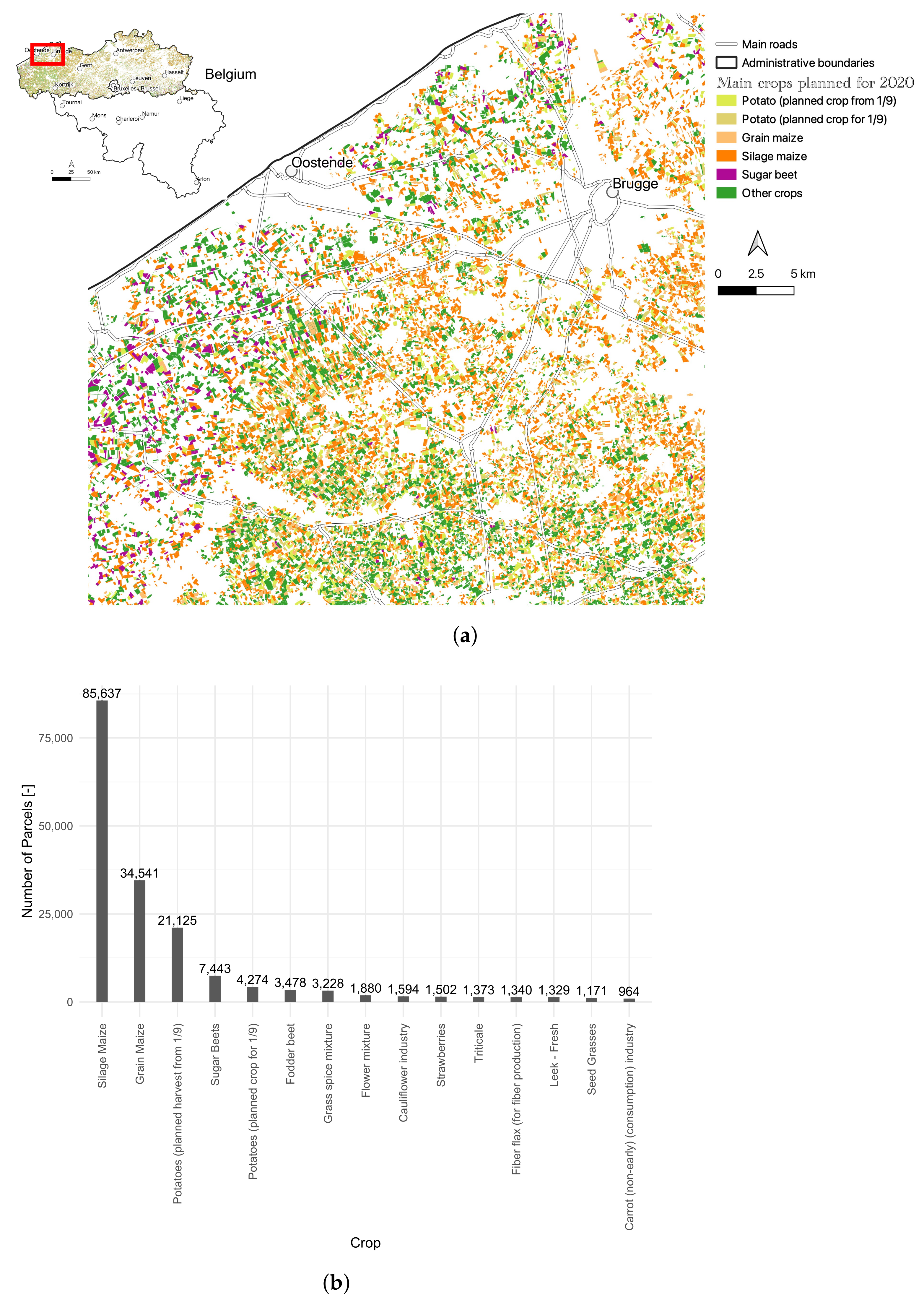
2.1. Study Area and the Agricultural Parcel Dataset

Since 1990, agriculture has accounted for an unchanged 45% of the land use in northern Belgium (Flanders). With a population density of 475 inhabitants per km${}^2$, the pressure on land is high; as a consequence agriculture is intensive and industrialised [6]. Agricultural land comprises 6,230 km${}^2$, out of which 70% is arable. Meadows, pastures, and fodder crops account for 56% of the total area in Flanders, and are a dominant land feature of the rural landscape. The largest portion of revenue is taken by intensive sectors such as pig breeding, poultry and dairy farming, horticulture, and ornamental plant culture.

The agricultural fields of Flanders are highly fragmented and relatively small, reaching in various cases less than 2 ha surface area with an average farm area of 15 ha [30]. A database of agricultural parcels compiled in 2020 was used, as parcels are annually documented in a regional database containing parcel surface area along with the planned major crop for the considered year. The database follows the procedures set by the Integrated Administration and Control System (IACS) of the European Common Agricultural Policy that aims to manage and control payments made by the member states to farmers. The extensive 2020 parcel dataset was filtered to exclude crops that were not expected to have a bare soil window between April and May, such as those with fruit and nut trees, winter grains, and grassland. The remaining selected crops were very diverse and dominated by maize, potatoes, and sugar beet (Figure 1).

Greenhouse horticulture is an important sub-sector in Flemish agriculture although it only represents an estimated 0.3% of the agricultural area [31]. The greenhouses (GHs) used for commercial activities can be made of plastic or glass with frames of metal, wood, etc. Various crops that heavily depend on greenhouse cultivation in northern Belgium include strawberries, small fruits, vegetables and leafy greens, along with floriculture where 35% of flower farming consists of greenhouses [31]. Farmers in Flanders also make use of diverse temporary covers for various purposes including weed suppression and soil warming. Soil care is central to agriculture, and a soil monitoring system is currently lacking. A simplified soil map (Figure 2) according to the World Reference Base for Soil Resources shows six reference soil groups, namely Cambisol (22%), Retisol (14%), Technosol (14%), Luvisol (13%), Podzol (12%), and Anthrosol (11%) [32], where Technosols are mostly associated with urban areas.

2.2. Sentinel-2 Imagery

The Copernicus Sentinel-2 two-satellite constellation (S2A and S2B) provides data acquired by the multispectral instruments (MSIs). The acquired imagery are freely available and reach a 5-day geometric revisit time. The MSI sensors provide images with thirteen bands where spatial resolution is band (B)-dependent and reaches 10m, 20m, or 60m [33] (

Table 1. Spatial resolution, central wavelength ($\lambda$), and bandwidth ($\delta \lambda$) of the two MSIs on board Sentinel-2 platforms.

Band	Resolution (m)	S2A		S2B
		$\mathit{\lambda }$ (nm)	$\mathit{\delta }\mathit{\lambda }$ (nm)	$\mathit{\lambda }$ (nm)	$\mathit{\delta }\mathit{\lambda }$ (nm)
B1	60	442.7	21	442.2	21
B2	10	492.4	66	492.1	66
B3	10	559.8	36	559.0	36
B4	10	664.6	31	664.9	31
B5	20	704.1	15	703.8	16
B6	20	740.5	15	739.1	15
B7	20	782.8	20	779.7	20
B8	10	832.8	106	832.9	106
B8a	20	864.7	21	864.0	22
B9	60	945.1	20	943.2	21
B10	60	1373.5	31	1376.9	30
B11	20	1613.7	91	1610.4	94
B12	20	2202.4	175	2185.7	185

). This new generation of freely available spaceborne acquisitions provides great new opportunities to monitor changes in soil cover at the parcel level in regions with small-patched units such as the parcels in the study area.

2.3. Data Pre-Processing

2.3.1. Overview

The data pre-processing aims at achieving high quality surface reflectance per pixel of a parcel with potential bare soil, and, thus, a combination of freely accessible tools was used for this purpose as shown in Figure 3. A time-series of Sentinel-2 imagery between mid-April and end-May was selected and pre-processed for a year of interest using Google Earth Engine (GEE), a cloud-based computing environment [34]. Further spatial data handling at the parcel- and pixel-level was carried out with R programming using various packages including sf [35], sp [36], rgdal [37], rgeos [38], Raster [39], SpatialEco [40], geojsonsf [41], and the tidyverse collection [42]. Spectral plots were prepared using the HyperSpec package [43].

2.3.2. Filtering Parcel Geometry

Sentinel-2 data have performed well in the context of monitoring small agricultural parcels [44] where a minimum surface area of 0.5 ha is recommended. Agricultural parcels in Flanders consist of units with various shapes and orientations. To reduce the number of mixed soil pixels at the boundaries, an inner buffer of 20 m was applied for each parcel, thus reducing further the parcel surface area. Different strategies were used to exclude parcels that could reduce data quality. Prior to buffering, parcels of complex and mainly elongated geometry that could result in lower accuracy [44] were identified and excluded. A shape index (SI) guided the identification (Equation (1)), where $SI=1$ resulted in a circular shape and increased for more elongated and complex geometrical shapes [45]. A threshold of SI of 2.5 was applied to exclude complex parcel geometries of higher values. After setting the parcel inner buffers, separate geometrical shapes could evolve from a one polygon parcel (Figure 4). These resulting polygons were segregated into individual geometries while they held the same parcel metadata. All resulting polygons with areas below $6000m^2$ were excluded.

$$SI=\frac{perimeter}{2\times \sqrt{\pi \times area}}$$

(1)

2.3.3. Pre-Processing of Sentinel-2 Data

The first essential task prior to analysing the Sentinel-2 imagery was the detection of clouds and their shadows, and subsequently excluding affected pixels. The direct use of cloud and shadow masks and quality bands available for Sentinel-2 data through Sen2Cor [46] were challenging as various clouds and shadows could be falsely omitted [47]. Using GEE, a collection of level (L)1C top of atmosphere (TOA) reflectance data covering Flanders were filtered to exclude those with cloud coverage exceeding 50% and were spatially mosaicked per acquisition date. A pixel-based approach was used where clouds and shadows were detected using the supervised classification of the quality bands (QA60) [48,49]. The high quality Sen2Cor-produced cirrus cloud masks [50] were also utilised.

To preserve a parcel’s spatial integrity, each parcel containing masked-out pixels was fully excluded from the corresponding acquisition date. Furthermore, to further detect any omitted clouds affecting the parcels, a multi-temporal approach comparing the acquisition dates to a clear reference date was utilised and considered sudden variations in surface reflectance in the red band (B4) and the blue band (B2) [51]. On the other hand, to detect omitted cloud shadows, their “darker” characteristics in the near- and shortwave infrared parts of the spectrum were considered [52] utilising the red band (B4) and the NIR band of 10m resolution (B8).

2.4. Acquisition-Date Selection per Parcel

Within the period from mid-April to end-May, a shadow- and cloud-free image of each parcel was required under potential bare soil conditions. NDVI (Equation (2)) with a limiting threshold of 0.3 was used to detect potentially bare soil where this threshold aligns with various studies using thresholds of 0.2 [13,53], 0.25 [11], 0.30 [54], or 0.35 [12].

$$NDVI=\frac{NIR-RED}{NIR+RED}=\frac{B8-B4}{B8+B4}$$

(2)

Trade-offs existed between the best image for each parcel in the time series while limiting the number of images with different acquisition dates to reduce the influence of acquisition conditions, such as sun illumination, soil moisture content, and other factors. Hereto a ranking of the available imagery was carried out based on the number of complete parcels available per date after clouds and shadow removal. Accordingly, each parcel’s bare soil pixels were selected from the corresponding highest-ranked acquisition date.

2.5. Anomaly Detection

For a functional dataset of bare soil, NDVI was not enough to extract uncovered agricultural parcels. The detection of anomalies was built upon the knowledge of bare soil characteristics in medium resolution spaceborne data. Supporting NDVI, green vegetation indices (GVI) (Equation (3)) were used, where values exceeding 0 have been attributed to bare soil pixels [11,12]. The soil-line (Red-NIR line) concept using near infrared and the red bands [14,55] was also used to identify major anomalies in the data, including various types of artificial covers. The Red-NIR line allowed a visual screening of the data, knowing that bare soil pixels were expected to follow a linear trend-line and were of relatively low reflectances [55]. High differences in inter-band reflectance in the visible part of the spectrum could also indicate the presence of anomalies. Sentinel-2 data includes three bands in the visible part of the spectrum at 10m resolution; the blue (BCC), green (GCC), and red (RCC) chromatic coordinates allowed the identification of such anomalies using Equation (4):

$$GVI1=B3-B2,GVI2=B4-B3$$

(3)

$$BCC=\frac{B2}{B2+B3+B4},GCC=\frac{B3}{B2+B3+B4},RCC=\frac{B4}{B2+B3+B4}$$

(4)

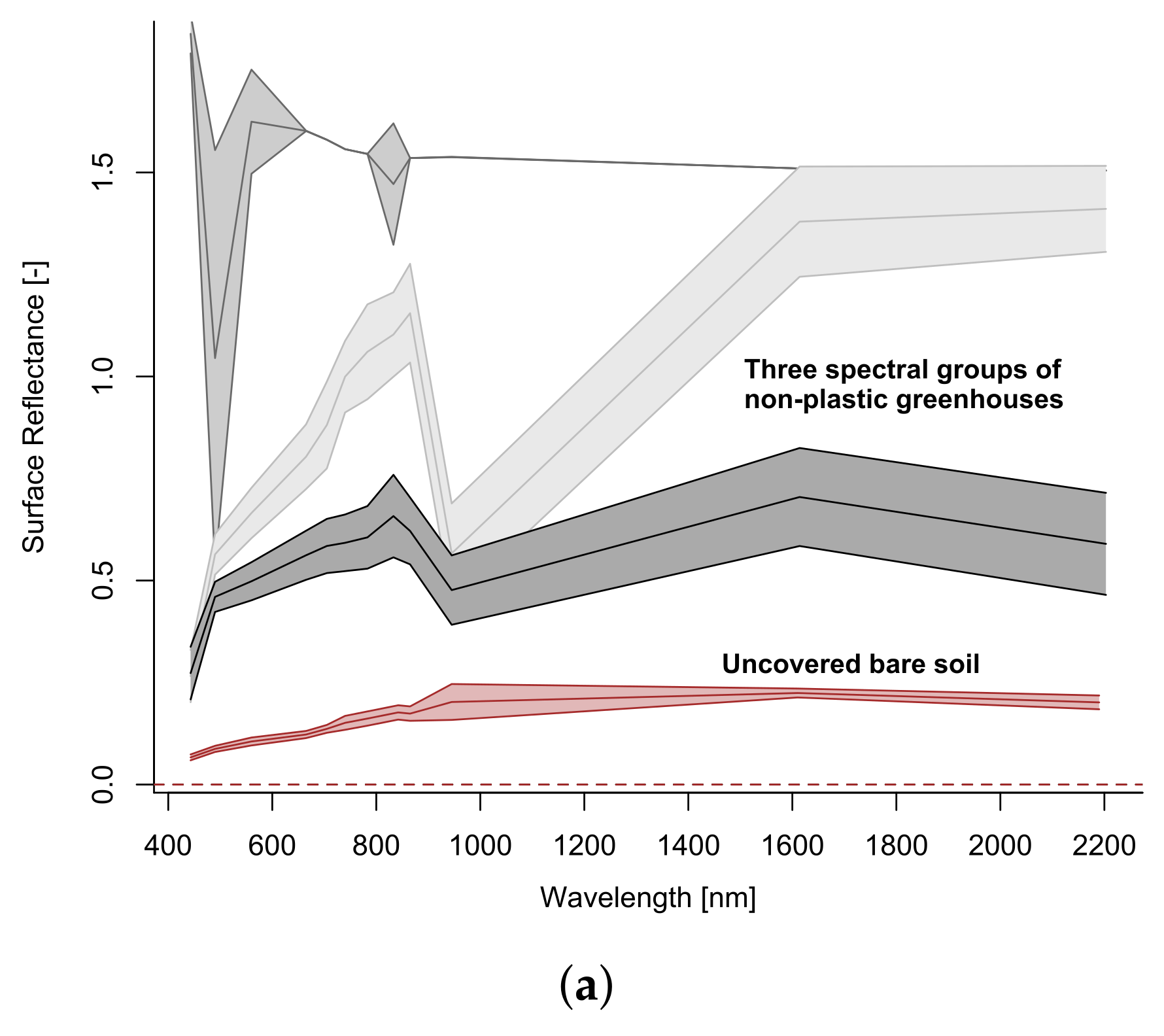
2.6. Large Non-Plastic Greenhouses and Temporary Soil Covers

As no inventory of covers in Flanders is available, nor is there a library of suitable reference spectra, the inspection of the detected anomalies provided diverse reference parcels and this opportunity to develop a machine-learning approach that identified other similarly covered sites. The spectra of non-plastic GHs and those of diverse soil covers had distinctive features from the underlying soil or crop. Although the spectra of various temporary soil covers, such as mulch films were highly impacted by the underlying soil, they were distinct from spectra of plastic GHs or uncovered bare soil (Figure 5). The spectral angle mapper (SAM) was used to identify such artificial covers using the hsdar package in R [56]. SAM measured the similarity among spectra to reference spectra and proved a powerful spectral distance approach used in various studies related to soil characterisation [57,58]. A spectrum is a vector in an n-dimensional space with n representing the number of considered bands. SAM resulted in an angle (in radians) as expressed in Equation (5). Since the target was to measure the angle between a reference vector and another, the vector length was not considered with SAM, making it a feature-based approach that does not consider overall brightness. This short-coming is not relevant to non-plastic GH detection and temporary soil covering films.

$$SAM=co{s}^{-1}\left(\frac{{\sum }_{i=1}^n{S}_i{R}_i}{\sqrt{{\sum }_{i=1}^n{S}_i^2}\sqrt{{\sum }_{i=1}^n{R}_i^2}}\right)$$

(5)

where $i\in [1,n]$, S is a reflectance spectrum to be analysed while R is a reference spectrum. Reference spectra of large permanent greenhouse structures and soil covers were identified through anomaly detection using the RED-NIR line, GVI1, and GVI2, and through visual inspection of satellite data.

The lower the angle, the similar the spectra are to each other, making it essential to assess a threshold’s suitability. With the presence of various types of greenhouses and cover films and with diverse spectra within each group, several reference spectra were needed, for which the angle was calculated separately. To create representative groups of reference spectra and extract end-members that provided computational efficiency, the vector length ($\left|\right|r\left|\right|$) of a reference spectrum was introduced (Equation (6)) as a quantitative metric to subset variable classes of representative end-members [59]. To define group end-members, spectra were partitioned into a number of equal intervals and a representative spectrum was achieved by calculating the mean spectrum of the subset. Various subset scenarios were tested for the choice of the end-members. The possible impacts of underlying soil groups on the detection of temporary covers was also considered. Reference spectra were compared for covered reference soil groups to corresponding uncovered pixels of all reference soil groups. Accordingly, decisions to split the dataset were made to detect the temporary cover per subset.

$$\left|\right|r\left|\right|=\sqrt{\sum _{i=1}^n{R}_i^2}$$

(6)

2.7. The Plastic Greenhouse Index

As plastic GHs are highly linked to the spectra of underlying crops or soils, their spectral features were expected to be similar yet with an overall higher reflectance. Thus, SAM, as a feature targeting approach, was not useful for the detection of such covers. The retrogressive plastic greenhouse index (RPGI) based on medium resolution multispectral imagery [18] was used for the detection of plastic GHs (Equation (7)). RPGI proved a robust measure for the binary selection of plastic GH pixels where NDVI < 0.73. However, this index has limitations, such as its dependency on the underlying vegetation and its low capability of detecting greenhouses in Summer when sheets are painted white [19], neither of which applied to our test area or temporal window. From the original development scenarios of the index on plastic greenhouses, a threshold of the index to derive a distinction between greenhouse pixels and others was tested and found to be a maximum of 1.6. We tested different threshold intervals, and a threshold based on graphical interpretation of the RPGI’s overall accuracy was accordingly selected.

$$RPGI=\frac{BLUE}{1-(RED+GREEN+NIR)/3}$$

(7)

2.8. Accuracy Assessment Using High Resolution Data

An area of approximately 30,000 ha was covered by high resolution imagery provided by Google Earth acquired on 11 April 2020 and was used for accuracy assessment of the results. The presence of artificial covers was inspected visually for each considered parcel. precision ($P_r$) and sensitivity ($S_p$) values were calculated: $P_r=T/(T+Fp)$, where T is the number of true positives and $Fp$ the number of false positives, and $S_p=T/(T+Fn)$, where $Fn$ is the number of false negatives. Furthermore, the knowledge of the expected crops to utilise greenhouses allowed a better assessment of results and the ease of detection of commission errors.

3. Results

3.1. Extracting Reflectance Information of Sentinel-2 for Agricultural Parcels

The clean-up of parcels based on crop types, geometries, and surface areas resulted in the retention of 66,665 parcels distributed among 173 planned crops for 2020. After excluding clouds and cloud shadows, the available number of valid pixels in the parcels of selected crops are shown in Figure 6a. The number of valid pixels varied in the temporal series, and a ranking of each date was carried out with respect to the number of valid parcels. Rank 1 was set for the data acquired on 20 April 2020, corresponding to the highest number of pixels (exceeding 17 million pixels). The corresponding number of parcels covered by each image is shown in Figure 6b, along with the remaining parcels after an NDVI threshold of 0.3. Rank 1 data provided 65,616 parcels of which 44,142 (67%) had a mean NDVI value < 0.3 for each parcel. The first three ranks were chosen and represented 99.1% of the parcels with NDVI < 0.3 (Figure 7).

Considering Rank 1 data, greenhouses that resulted in major anomalies in the parcel dataset are well visible in the RED-NIR scatter of Rank 1 pixels subjected to the NDVI threshold of 0.3 (Figure 8). The major segment of the data followed the expected line for bare soil and was mainly clustered around the lower reflectance. Very high reflectances, even exceeding 1, were observed for both NIR and RED, indicating the presence of high specular reflection.

Values exceeding 0.75 in B4 were of 345 pixels of non-plastic greenhouses that were planned for planting tomatoes, strawberries, strawberry seedlings, and rucola, and had distinct reflectance spectra when compared to bare soil (Figure 9). All parcels containing an identified anomaly were excluded, resulting in the loss of four parcels and 508 pixels. Such a relatively small number of pixels highly affected the RED-NIR line and emphasised the need to address such anomalies in soil data.

GVI1 and GVI2 values below 0 corresponded to pixels of diverse artificial soil covers from greenhouses to thin temporary films (Figure 10). This was confirmed by high resolution imagery provided by Google Earth including an acquisition on 11 April 2020, i.e., 9 days prior to the Rank 1 acquisition. These identified parcels were utilised as reference spectra for the detection of other covered parcels.

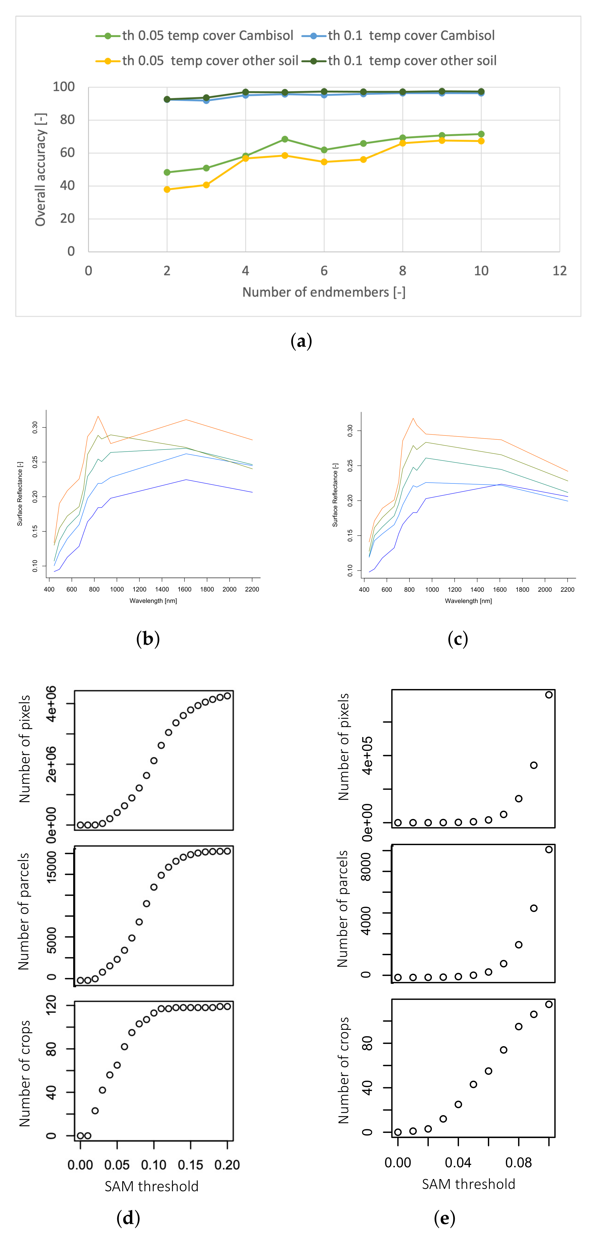
3.2. Temporary Covers on Various Soil Types

As underlying soil impacts the reflectance of the temporary covers, especially mulch films, reference spectra of covered sections were compared to non-covered sections. $\left|\right|r\left|\right|$ was calculated for each spectrum to simplify dimensionality for broccoli, cabbage, carrots, and maize (Figure 11). These plots illustrated the distinctive reflectance of covered soil, except for the case of Cambisols (Figure 11b) where covered pixels were overlapping with $\left|\right|r\left|\right|$ values of other soil types. Cambisols were separated, and the temporary cover detection was carried out on each subset.

3.3. Detection of Covered Parcels by SAM and RPGI

A collection of 3575 pixels of 14 parcels and 10 crops were the reference to detect temporary covers. Thresholds of 0.05 and 0.1 were tested where the overall accuracy was reported for each different scenario (Figure 12a). Accordingly, 5 end-members (Figure 12b,c) were chosen for each subset of soil groups where they showed relatively high detection capability. Selected thresholds were 0.012 and 0.04 for Cambisol and others, respectively, where these thresholds set a boundary for a major increase in commissioned crop types and crops (Figure 12d,e).

For non-plastic greenhouses, 1,396 pixels corresponding to 7 parcels and 6 crop were used as reference. SAM was able to identify at least one pixel in each parcel and crop-type using a threshold of 0.1 or higher starting from 2 end-members (Figure 13). To identify all pixels (achieving 100% overall accuracy) a threshold exceeding 0.2 would be needed. With the increase in the number of end-members, the overall accuracy of parcels increased at lower threshold values, but the overall accuracy of pixels did not significantly improve. This confirmed the challenge with such greenhouse detection as there was a large variability in the spectra within the same parcel. Four end-members were selected with a threshold of 0.06 that resulted in the omission of one reference parcel (Figure 13g).

Figure 14 shows the number of pixels, parcels, and crops attributed to plastic greenhouses for a range of RPGI thresholds. RPGI = 0.4 represented a major breaking point in the attribution of pixels to plastic greenhouses, and thus RPGI > 0.4 was used for the detection on such greenhouses.

3.4. Detailing the Crops That Utilise Artificial Covers

Once a pixel was flagged as covered, all pixels in the corresponding parcel were also labelled as such and excluded from the potential bare soil database. An overview of identified covered pixels and corresponding crops are shown in Figure 15, where 20,626 pixels were attributed to temporary covers, 4,198 pixels to non-plastic greenhouses, and 13,401 to plastic greenhouses.

3.4.1. Accuracy Assessment of Artificial Cover Detection Using High Resolution Data

The high resolution data around the centre of Flanders included approximately 46,450 agricultural parcels of Rank 1 imagery. The detected artificial covers are shown in Figure 16. The area included only 1 parcel with plastic greenhouses that was successfully detected, yet another parcel with a visual anomaly on the borders was commissioned, resulting in a relatively lower $P_r$ value. Furthermore, a number of partially covered parcels with mulch films were not captured, resulting in the relatively lower $S_p$ value for the temporary covers. There was a very limited number of false positives, resulting in an overall high $S_p$ of the approach (Figure 16).

3.4.2. Excluding Miscellaneous Anomalies

After the exclusion of all greenhouse pixels, the chromatic coordinates (CC) were used to detect any additional anomalies in the visible part of the spectrum, identifying non-detected artificial covers. Figure 17 shows a boxplot with all pixels and outliers that were considered as anomalies, where CCs were retained, such that $0.15<BCC<0.325$, $0.25<GCC<0.375$, $0.325<RCC<0.55$. The excluded values referred to non-detected mulch covers, anomalies in the field that could most likely be attributed to farm vehicles, and a number of parcel-border pixels that were retained after buffering.

3.4.3. Detection of Artificial Covers in the Time-Series

The methodology to detect artificial soil covers illustrated for Rank 1 data was carried out for two subsequent ranks to cover the majority of agricultural parcels. Figure 18 shows all the detected artificial covers and an overview of their proportions. Figure 19 shows an update of the RED-NIR scatter for pixels excluding these anomalies for Rank 1, a composite of Rank 1 with Rank 2, and a composite of all the first three ranks. Figure 20 shows an overview of the crops with detected soil covers for the first three ranks of acquisition dates.

4. Discussion

Powerful approaches to detect bare soil have been already developed for Landsat, Sentinel-2, and a combination of sensors [11,54,60], and have successfully mapped large areas to analyse soil characteristics. These approaches focus on merging data within the time series at pixel level, aiming to reduce the occurrence of extreme reflectances and to obtain stable and representative values. The methodology developed in this paper preserves an agricultural parcel’s spatial and temporal integrity and highlights the interpretation of anomalies and extreme values. These aspects allow the yearly mapping of parcels and provide insights on soil surface characteristics to the land-managers at the parcel level. Furthermore, they set the foundation for the development of suitable monitoring strategies for agricultural soil and provide the possibility to plan in-situ field campaigns and surveys.

The NDVI, GVI1, GVI2 thresholds to identify potentially bare soil were in tune with other research seeking bare soil spectra [10,11,12,61]. As the focus was only on agricultural parcels, GVI1 and GVI2 were important indicators for the presence of artificial covers. Agricultural parcels with artificial covers were relatively low in area and in number, yet they highly affected the data and, therefore, compromised the understanding of soil surface characteristics and patterns based on spectral signatures. The RED-NIR line allowed for the detection of those anomalies due to their known patterns in bare soil spectra [62]. The resulting cleaned data provided an improved dataset for subsequent cover analysis and monitoring. For example, using the RED-NIR line concept, higher values could represent straw and post-harvest residues [55]. Detected anomalies provided a valuable dataset of reference spectra of various soil covers. Furthermore, the time-series revealed land preparation activities where the fraction of parcels with a low NDVI was highest around the middle of the considered period when comparing the first three ranked dates of image acquisitions, i.e., 17 April, 15 May, and 30 May.

SAM was used for the detection of temporary covers and non-plastic greenhouses. The choice of end-members along with the selected constraints highly impacted the results in such a spectral matching approach. The constraints used by SAM were assessed by calculating the fraction of correct detection of artificial covers on pixels, parcels, and crops using various scenarios of end-members. With the increase in the angle, the detection of the covered pixels was increasing [63]. A trade-off existed between precision and sensitivity as with the increase in threshold to attain 100% accuracy, commission errors could increase. This is mainly due to the presence of diverse spectra in a covered parcel, especially for non-plastic greenhouses. A parcel could be labelled as covered once a pixel in the parcel was labelled, allowing higher constraints on the SAM angle and reducing commission errors.

Temporary covers in the considered period were limited to scattered parcels spread across the region, requiring high precision and sensitivity of the detection method. This setting has rarely been addressed in literature as typical study areas are extensively covered [27,64,65]. Research has emphasised the impact of diverse aspects, such as underlying soil or vegetation, the presence of dew on the cover, and the type of plastic material [24,28]. In our study, the underlying soil effects on the spectra of covered pixels was considered, and the spectra of covered areas were distinctly different from bare soil. Cambisols were best analysed separately, and accordingly, the spectral angle mapper resulted in high precision of the detection. The crops where these covers were identified included maize, root crops, and brassicas (Figure 15). The detection of artificial covers is crucial to agricultural waste management and a starting point to prioritise areas of micro-plastic residues in agricultural soil.

Non-plastic greenhouses showed major anomalies in the data including very high surface reflectances, indicating the presence of high specular reflection [66]. Both plastic and non-plastic greenhouses are challenging to detect using pixel-based approaches due to the heterogeneity of the spectra within the same greenhouse. There was the impact of the underlying structure and crops in the case of the large non-plastic greenhouses, while for the plastic greenhouses, there was the impact of borders around each greenhouse. Due to those reasons, researchers have suggested the use of object-based approaches [67]. Since the integrity of each parcel was preserved, the pixel-based approach was also powerful where once pixels were labelled as greenhouse pixels, the corresponding parcels were labelled accordingly. SAM was used for identifying non-plastic greenhouses, while revealing their scattered locations and their planned crops for 2020 with a dominant presence of strawberry cultivation. Plastic greenhouses resulted in spectra with high similarities to bare-soil spectra, thus the RPGI index was used for their detection. A suitable RPGI threshold was 0.4 emphasising the high mixed content of the pixels where the plastic greenhouses were estimated to represent 50% of a pixel’s content while the rest was attributed to the surroundings [18]. Plastic greenhouses were limited in number during the considered temporal window and represented only 18% of all detected covers with major usage for carrots.

The top three ranked acquisition days provided 99.1% of the parcels with NDVI < 0.3 in the considered window, emphasising the reliability of the approach at different acquisition conditions. Our approach sets a foundation for analysing time-series of multiple years and monitoring of the use of artificial covers and their trends [22]. Compositing the data acquired from the three dates while preserving each parcel’s spatial and temporal integrity resulted in a database of bare soil parcels ready for further analysis and in-line with the expected RED-NIR line representation (Figure 19). Various anomalies were also excluded from the data and were mainly attributed to parcel borders. The insights on temporary covers from three acquisition dates allowed mapping all artificial soil covers detected in the considered window (Figure 18) and revealed that artificial covers occurred most frequently in maize parcels (Figure 20).

5. Conclusions

We developed a methodology to identify potential bare soil pixels in uncovered agricultural parcels during the onset of cultivation when light conditions are optimal for further spectral analysis. We tested the methodology on Flanders, the northern region of Belgium, for the period mid April to end May when highly active agricultural management practices can leave the soil bare in preparation for main cropping seasons. The methodology provided a workflow to extract potentially bare soil by excluding the impacts of clouds, shadow, vegetated areas, and artificial soil covers in the dataset while preserving a parcel’s spatial and temporal integrity.

The spectral angle mapper was used along with a plastic greenhouse index to identify various types of artificial covers, namely temporary soil covers, non-plastic greenhouses, and plastic greenhouses. The approach resulted in the detection of temporary covers and non-plastic greenhouses with $P_r$ exceeding 0.9, showing the low commission errors of the approach, while resulting in low $P_r$ for plastic greenhouses due to their low numbers in the study area and in the considered period. The approach achieved higher $S_p$ values for non-plastic and plastic greenhouses indicating a good detection, while $S_p$ for temporary covers was around 0.7.

The approach presented in this paper provides a foundation to serve the dual purpose of characterising bare soil and identifying soil cover types of artificially covered agricultural parcels. The presented approach and resulting database provide a tool for setting up detailed soil analysis and monitoring programmes. The identification of soil covers, including plastic mulch, provides new insights on agricultural management practices, contributes to agricultural waste management, and can support prioritisation of areas with potential mulch residues and micro-plastics in the soil. GEE’s cloud computing platform along with Sentinel-2’s freely available data have been supports to a great transformation in digital agriculture, and this work contributes to this transformation.

References

1. McBratney, A.; Field, D.J.; Koch, A. The dimensions of soil security. Geoderma 2014, 213, 203–213. [Google Scholar] [CrossRef] [Green Version]
2. Hengl, T.; De Jesus, J.M.; Heuvelink, G.B.; Gonzalez, M.R.; Kilibarda, M.; Blagotić, A.; Shangguan, W.; Wright, M.N.; Geng, X.; Bauer-Marschallinger, B.; et al. SoilGrids250m: Global gridded soil information based on machine learning. PLoS ONE 2017, 12, e169748. [Google Scholar] [CrossRef] [PubMed] [Green Version]
3. Durgun, Y.O.; Gobin, A.; Van De Kerchove, R.; Tychon, B. Crop Area Mapping Using 100-m Proba-V Time Series. Remote Sens. 2016, 8, 585. [Google Scholar] [CrossRef] [Green Version]
4. Marshall, M.; Crommelinck, S.; Kohli, D.; Perger, C.; Yang, M.Y.; Ghosh, A.; Fritz, S.; de Bie, K.; Nelson, A. Crowd-driven and automated mapping of field boundaries in highly fragmented agricultural landscapes of Ethiopia with very high spatial resolution imagery. Remote Sens. 2019, 11, 2082. [Google Scholar] [CrossRef] [Green Version]
5. Van Tricht, K.; Gobin, A.; Gilliams, S.; Piccard, I. Synergistic Use of Radar Sentinel-1 and Optical Sentinel-2 Imagery for Crop Mapping: A Case Study for Belgium. Remote Sens. 2018, 10, 1642. [Google Scholar] [CrossRef] [Green Version]
6. Vannoppen, A.; Gobin, A. Estimating Farm Wheat Yields from NDVI and Meteorological Data. Agronomy 2021, 11, 946. [Google Scholar] [CrossRef]
7. Tenkorang, F.; Lowenberg-DeBoer, J. On-Farm Profitability of Remote Sensing in Agriculture. J. Terr. Obs. 2008, 1, 6. [Google Scholar]
8. Saiz-Rubio, V.; Rovira-Más, F. From smart farming towards agriculture 5.0: A review on crop data management. Agronomy 2020, 10, 207. [Google Scholar] [CrossRef] [Green Version]
9. Weiss, M.; Jacob, F.; Duveiller, G. Remote sensing for agricultural applications: A meta-review. Remote Sens. Environ. 2020, 236, 111402. [Google Scholar] [CrossRef]
10. Castaldi, F.; Palombo, A.; Santini, F.; Pascucci, S.; Pignatti, S.; Casa, R. Evaluation of the potential of the current and forthcoming multispectral and hyperspectral imagers to estimate soil texture and organic carbon. Remote Sens. Environ. 2016, 179, 54–65. [Google Scholar] [CrossRef]
11. Demattê, J.; Troula, C.; Rizzo, R.; Lucas, J. Remote Sensing of Environment Geospatial Soil Sensing System (GEOS3): A powerful data mining procedure to retrieve soil spectral re fl ectance from satellite images. Remote Sens. Environ. 2018, 212, 161–175. [Google Scholar] [CrossRef]
12. Castaldi, F.; Chabrillat, S.; Don, A.; van Wesemael, B. Soil organic carbon mapping using LUCAS topsoil database and Sentinel-2 data: An approach to reduce soil moisture and crop residue effects. Remote Sens. 2019, 11, 2121. [Google Scholar] [CrossRef] [Green Version]
13. Mzid, N.; Pignatti, S.; Huang, W.; Casa, R. An analysis of bare soil occurrence in arable croplands for remote sensing topsoil applications. Remote Sens. 2021, 13, 474. [Google Scholar] [CrossRef]
14. Nguyen, C.T.; Chidthaisong, A.; Kieu Diem, P.; Huo, L.Z. A Modified Bare Soil Index to Identify Bare Land Features during Agricultural Fallow-Period in Southeast Asia Using Landsat 8. Land 2021, 10, 231. [Google Scholar] [CrossRef]
15. Rogge, D.; Bauer, A.; Zeidler, J.; Mueller, A.; Esch, T.; Heiden, U. Remote Sensing of Environment Building an exposed soil composite processor (SCMaP) for mapping spatial and temporal characteristics of soils with Landsat imagery (1984–2014). Remote Sens. Environ. 2018, 205, 1–17. [Google Scholar] [CrossRef] [Green Version]
16. Aguilar, M.A.; Vallario, A.; Aguilar, F.J.; Lorca, A.G.; Parente, C. Object-based greenhouse horticultural crop identification from multi-temporal satellite imagery: A case study in Almeria, Spain. Remote Sens. 2015, 7, 7378–7401. [Google Scholar] [CrossRef] [Green Version]
17. Novelli, A.; Aguilar, M.A.; Nemmaoui, A.; Aguilar, F.J.; Tarantino, E. Performance evaluation of object based greenhouse detection from Sentinel-2 MSI and Landsat 8 OLI data: A case study from Almería (Spain). Int. J. Appl. Earth Obs. Geoinf. 2016, 52, 403–411. [Google Scholar] [CrossRef] [Green Version]
18. Yang, D.; Chen, J.; Zhou, Y.; Chen, X.; Chen, X.; Cao, X. Mapping plastic greenhouse with medium spatial resolution satellite data: Development of a new spectral index. ISPRS J. Photogramm. Remote Sens. 2017, 128, 47–60. [Google Scholar] [CrossRef]
19. Nemmaoui, A.; Aguilar, M.A.; Aguilar, F.J.; Novelli, A.; Lorca, A.G. Greenhouse crop identification from multi-temporal multi-sensor satellite imagery using object-based approach: A case study from Almería (Spain). Remote Sens. 2018, 10, 1751. [Google Scholar] [CrossRef] [Green Version]
20. González-Yebra, Ó.; Aguilar, M.A.; Nemmaoui, A.; Aguilar, F.J. Methodological proposal to assess plastic greenhouses land cover change from the combination of archival aerial orthoimages and Landsat data. Biosyst. Eng. 2018, 175, 36–51. [Google Scholar] [CrossRef]
21. Jiménez-Lao, R.; Aguilar, F.J.; Nemmaoui, A.; Aguilar, M.A. Remote sensing of agricultural greenhouses and plastic-mulched farmland: An analysis of worldwide research. Remote Sens. 2020, 12, 2649. [Google Scholar] [CrossRef]
22. Ou, C.; Yang, J.; Du, Z.; Liu, Y.; Feng, Q.; Zhu, D. Long-term mapping of a greenhouse in a typical protected agricultural region using landsat imagery and the google earth engine. Remote Sens. 2020, 12, 55. [Google Scholar] [CrossRef] [Green Version]
23. Koc-San, D.; Sonmez, N.K. Plastic and glass greenhouses detection and delineation from WorldView-2 satellite imagery. In Proceedings of the International Archives of the Photogrammetry, Remote Sensing and Spatial Information Sciences—ISPRS, 2016 XXIII ISPRS Congress, Prague, Czech Republic, 12–19 July 2016; Archives: Prague, Czech Republic, 2016; Volume 41, pp. 257–262. [Google Scholar] [CrossRef]
24. Levin, N.; Lugassi, R.; Ramon, U.; Braun, O.; Ben-Dor, E. Remote sensing as a tool for monitoring plasticulture in agricultural landscapes. Int. J. Remote Sens. 2007, 28, 183–202. [Google Scholar] [CrossRef]
25. Lanorte, A.; De Santis, F.; Nolè, G.; Blanco, I.; Loisi, R.V.; Schettini, E.; Vox, G. Agricultural plastic waste spatial estimation by Landsat 8 satellite images. Comput. Electron. Agric. 2017, 141, 35–45. [Google Scholar] [CrossRef]
26. Pereira, A.R.; Hernandez, A.; James, B.; Lemoine, B.; Carranca, C.; Rayns, F.; Cornelis, G.; Erälinna, L.; Czech, L.; Minipaper A: The Actual Uses of Plastics in Agriculture across EU: An Overview and the Environmental Problems. Technical Report February, EIP-AGRI Focus Group Reducing the Plastic Footprint of Agriculture Overview and the Environmental Problems. 2021. Available online: https://ec.europa.eu/eip/agriculture/en/publications/eip-agri-focus-group-plastic-footprint-final (accessed on 19 October 2021).
27. Lu, L.; Di, L.; Ye, Y. A decision-tree classifier for extracting transparent plastic-mulched Landcover from landsat-5 TM images. IEEE J. Sel. Top. Appl. Earth Obs. Remote Sens. 2014, 7, 4548–4558. [Google Scholar] [CrossRef]
28. Xiong, Y.; Zhang, Q.; Chen, X.; Bao, A.; Zhang, J.; Wang, Y. Large scale agricultural plastic mulch detecting and monitoring with multi-source remote sensing data: A case study in Xinjiang, China. Remote Sens. 2019, 11, 2088. [Google Scholar] [CrossRef] [Green Version]
29. Lu, L.; Tao, Y.; Di, L. Object-based plastic-mulched landcover extraction using integrated Sentinel-1 and Sentinel-2 data. Remote Sens. 2018, 10, 1820. [Google Scholar] [CrossRef] [Green Version]
30. Vannoppen, A.; Degerickx, J.; Gobin, A. Evaluating Landscape Attractiveness with Geospatial Data, A Case Study in Flanders, Belgium. Land 2021, 10, 703. [Google Scholar] [CrossRef]
31. Platteau, J.; Lambrechts, G.; Roels, K.; Van Bogaert, T.; Luypaert, G.; Merckaert, B. Challenges for Flemish Agriculture and Horticulture, Technical Report; Department of Agriculture and Fisheries: Brussels, Belgium, 2018. [Google Scholar]
32. Dondeyne, S.; Vanierschot, L.; Langohr, R.; Ranst, E.V.; Deckers, J. The Soil Map of the Flemish Region Converted to the 3rd Edition of the World Reference Base for soil Resources; Technical Report; Onderzoek Uitgevoerd in Opdracht van de Vlaamse Overheid; Departement Leefmilieu, Natuur en Energie Afdeling Land en Bodembescherming, Ondergrond, Natuurlijke Rijkdommen: Brussels, Belgium., 2014. [Google Scholar]
33. Drusch, M.; Del Bello, U.; Carlier, S.; Colin, O.; Fernandez, V.; Gascon, F.; Hoersch, B.; Isola, C.; Laberinti, P.; Martimort, P.; et al. Sentinel-2: ESA’s Optical High-Resolution Mission for GMES Operational Services. Remote Sens. Environ. 2012, 120, 25–36. [Google Scholar] [CrossRef]
34. Gorelick, N.; Hancher, M.; Dixon, M.; Ilyushchenko, S.; Thau, D.; Moore, R. Google Earth Engine: Planetary-scale geospatial analysis for everyone. Remote Sens. Environ. 2017, 202, 18–27. [Google Scholar] [CrossRef]
35. Pebesma, E. Simple Features for R: Standardized Support for Spatial Vector Data. R J. 2018, 10, 439–446. [Google Scholar] [CrossRef] [Green Version]
36. Pebesma, E.J.; Bivand, R.S. Classes and methods for spatial data in R. R News 2005, 5, 9–13. [Google Scholar]
37. Bivand, K.; Keitt, T.; Rowlingson, B.; Pebesma, E.; Sumner, M.; Hijmans, R.; Baston, D.; Rouault, E.; Warmerdam, F.; Ooms, J.; et al. Rrgdal: Bindings for the ’Geospatial’ Data Abstraction Library. 2021. Available online: https://cran.r-project.org/web/packages/rgdal/index.html (accessed on 19 October 2021).
38. Bivand, R.; Rundel, C.; Rgeos: Interface to Geometry Engine—Open Source (’GEOS’). R Package Version 0.5-3. 2020. Available online: https://CRAN.R-project.org/package=rgeos (accessed on 19 October 2021).
39. Van Etten, R.J.H.J. Raster: Geographic Analysis and Modeling with Raster Data. R Package Version 2.0-12. 2012. [Google Scholar]
40. Evans, J.S. spatialEco, R Package Version 1.3-6. 2021. Available online: https://cran.r-project.org/web/packages/spatialEco/index.html (accessed on 19 October 2021).
41. Cooley, D. Geojsonsf: GeoJSON to Simple Feature Converter. 2019. Available online: https://CRAN.R-project.org/package=geojsonsf (accessed on 19 October 2021).
42. Wickham, H.; Averick, M.; Bryan, J.; Chang, W.; McGowan, L.D.; François, R.; Grolemund, G.; Hayes, A.; Henry, L.; Hester, J.; et al. Welcome to the tidyverse. J. Open Source Softw. 2019, 4, 1686. [Google Scholar] [CrossRef]
43. Beleites, C.; Sergo, V. hyperSpec: A Package to Handle Hyperspectral Data Sets in R. version 0.100. Available online: https://cran.r-project.org/web/packages/hyperSpec/hyperSpec.pdf (accessed on 19 October 2021).
44. Vajsová, B.; Fasbender, D.; Wirnhardt, C.; Lemajic, S.; Devos, W. Assessing spatial limits of Sentinel-2 data on arable crops in the context of checks by monitoring. Remote Sens. 2020, 12, 2195. [Google Scholar] [CrossRef]
45. Comber, A.J.; Birnie, R.V.; Hodgson, M. A retrospective analysis of land cover change using a polygon shape index. Glob. Ecol. Biogeogr. 2003, 12, 207–215. [Google Scholar] [CrossRef] [Green Version]
46. Louis, J.; Debaecker, V.; Pflug, B.; Main-Knorn, M.; Bieniarz, J.; Mueller-Wilm, U.; Cadau, E.; Gascon, F. Sentinel-2 SEN2COR: L2A Processor for Users; European Space Agency, (Special Publication) ESA SP:, 2016; Volume SP-740, pp. 9–13. Available online: https://elib.dlr.de/107381/1/LPS2016_sm10_3louis.pdf (accessed on 19 October 2021).
47. Ibrahim, E.; Jiang, J.; Lema, L.; Barnab, P.; Giuliani, G.; Lacroix, P.; Pirard, E. Cloud and Cloud-Shadow Detection for Applications in Mapping Small-Scale Mining in Colombia Using Sentinel-2 Imagery. Remote Sens. 2021, 13, 736. [Google Scholar] [CrossRef]
48. Coluzzi, R.; Imbrenda, V.; Lanfredi, M.; Simoniello, T. A first assessment of the Sentinel-2 Level 1-C cloud mask product to support informed surface analyses. Remote Sens. Environ. 2018, 217, 426–443. [Google Scholar] [CrossRef]
49. Nguyen, M.D.; Baez-Villanueva, O.M.; Bui, D.D.; Nguyen, P.T.; Ribbe, L. Harmonization of landsat and sentinel 2 for crop monitoring in drought prone areas: Case studies of Ninh Thuan (Vietnam) and Bekaa (Lebanon). Remote Sens. 2020, 12, 281. [Google Scholar] [CrossRef] [Green Version]
50. Baetens, L.; Desjardins, C.; Hagolle, O. Validation of Copernicus Sentinel-2 Cloud Masks Obtained from MAJA, Sen2Cor, and FMask Processors Using Reference Cloud Masks Generated with a Supervised Active Learning Procedure. Remote Sens. 2019, 11, 433. [Google Scholar] [CrossRef] [Green Version]
51. Hagolle, O.; Huc, M.; Desjardins, C.; Auer, S.; Richter, R. MAJA Algorithm Theoretical Basis Document. 2017. Available online: https://doi.org/10.5281/zenodo.1209633 (accessed on 19 October 2021).
52. Zhu, Z.; Woodcock, C. Object-based cloud and cloud shadow detection in LANDSAT imagery. Remote Sens. Environ. 2012, 118, 83–94. [Google Scholar] [CrossRef]
53. Shabou, M.; Mougenot, B.; Chabaane, Z.L.; Walter, C.; Boulet, G.; Aissa, N.B.; Zribi, M. Soil clay content mapping using a time series of Landsat TM data in semi-arid lands. Remote Sens. 2015, 7, 6059–6078. [Google Scholar] [CrossRef] [Green Version]
54. Safanelli, J.L.; Chabrillat, S.; Ben-Dor, E.; Demattê, J.A. Multispectral models from bare soil composites for mapping topsoil properties over Europe. Remote Sens. 2020, 12, 1369. [Google Scholar] [CrossRef]
55. Koroleva, P.V.; Rukhovich, D.I.; Rukhovich, A.D.; Rukhovich, D.D.; Kulyanitsa, A.L.; Trubnikov, A.V.; Kalinina, N.V.; Simakova, M.S. Location of Bare Soil Surface and Soil Line on the RED—NIR Spectral Plane. Eurasian Soil Sci. 2017, 50, 1375–1385. [Google Scholar] [CrossRef]
56. Lehnert, L.W.; Meyer, H.; Obermeier, W.A.; Silva, B.; Regeling, B.; Thies, B.; Bendix, J. Hyperspectral Data Analysis in R: The hsdar Package. J. Stat. Softw. 2019, 89, 1–23. [Google Scholar] [CrossRef] [Green Version]
57. Sayão, V.M.; Demattê, J.A. Soil texture and organic carbon mapping using surface temperature and reflectance spectra in Southeast Brazil. Geoderma Reg. 2018, 14, e00174. [Google Scholar] [CrossRef]
58. Zeng, R.; Rossiter, D.G.; Zhao, Y.G.; Li, D.C.; Zhang, G.L. Forensic soil source identification: Comparing matching by color, vis-NIR spectroscopy and easily-measured physio-chemical properties. Forensic Sci. Int. 2020, 317, 110544. [Google Scholar] [CrossRef] [PubMed]
59. Xu, Y.; Shi, J.; Du, J. An improved endmember selection method based on vector length for MODIS reflectance channels. Remote Sens. 2015, 7, 6280–6295. [Google Scholar] [CrossRef] [Green Version]
60. Silvero, N.E.Q.; Demattê, J.A.M.; Amorim, M.T.A.; dos Santos, N.V.; Rizzo, R.; Safanelli, J.L.; Poppiel, R.R.; de Sousa Mendes, W.; Bonfatti, B.R. Soil variability and quantification based on Sentinel-2 and Landsat-8 bare soil images: A comparison. Remote Sens. Environ. 2021, 252, 112117. [Google Scholar] [CrossRef]
61. Casa, R.; Castaldi, F.; Pascucci, S.; Palombo, A.; Pignatti, S. A comparison of sensor resolution and calibration strategies for soil texture estimation from hyperspectral remote sensing. Geoderma 2013, 197–198, 17–26. [Google Scholar] [CrossRef]
62. Demattê, J.A.M.; Safanelli, J.L.; Poppiel, R.R.; Rizzo, R.; Silvero, N.E.Q.; Mendes, W.D.S.; Bonfatti, B.R.; Dotto, A.C.; Salazar, D.F.U.; Mello, F.A.D.O.; et al. Bare Earth’s Surface Spectra as a Proxy for Soil Resource Monitoring. Sci. Rep. 2020, 10, 4461. [Google Scholar] [CrossRef]
63. Dennison, P.E.; Halligan, K.Q.; Roberts, D.A. A comparison of error metrics and constraints for multiple endmember spectral mixture analysis and spectral angle mapper. Remote Sens. Environ. 2004, 93, 359–367. [Google Scholar] [CrossRef]
64. Picuno, P.; Tortora, A.; Capobianco, R.L. Analysis of plasticulture landscapes in Southern Italy through remote sensing and solid modelling techniques. Landsc. Urban Plan. 2011, 100, 45–56. [Google Scholar] [CrossRef]
65. Sun, H.; Wang, L.; Lin, R.; Zhang, Z.; Zhang, B. Mapping plastic greenhouses with two-temporal sentinel-2 images and 1d-cnn deep learning. Remote Sens. 2021, 13, 2820. [Google Scholar] [CrossRef]
66. Tan, K.; Cheng, X. Specular reflection effects elimination in terrestrial laser scanning intensity data using Phong model. Remote Sens. 2017, 9, 853. [Google Scholar] [CrossRef] [Green Version]
67. Wu, C.F.; Deng, J.S.; Wang, K.; Ma, L.G.; Tahmassebi, A.R.S. Object-based classification approach for greenhouse mapping using Landsat-8 imagery. Int. J. Agric. Biol. Eng. 2016, 9, 79–88. [Google Scholar] [CrossRef]
Figure 1. An overview of the selected crops in the 2020 database of Flanders, Belgium. (a) Agricultural parcels with potential bare soil between mid April and end of May and a close look at a subset region. (b) The major 15 crops with the highest number of parcels.
Remotesensing 13 04195 g001
Figure 2. Reference soil groups in Flanders (data source: [32]).
Remotesensing 13 04195 g002
Figure 3. Overview of the major preprocessing steps to achieve high quality reflectance per pixel of parcels with potential bare soil.
Remotesensing 13 04195 g003
Figure 4. An example of a parcel polygon (SI is 1.61), resulting in two separate polygon geometries due to a 20 m inner buffer.
Remotesensing 13 04195 g004
Figure 5. Examples of plastic and non-plastic greenhouse pixels, temporarily covered soil, and uncovered soil pixels, all satisfying NDVI < 0.3. The spectral plots show the mean and standard deviation per band considering 250 spectra for each group. The spectra were extracted from Sentinel-2 data acquired on 20 April 2020.
Remotesensing 13 04195 g005
Figure 6. Sentinel-2 acquisitions from mid-April to end-May and the corresponding valid data. (a) The number of valid parcel pixels and the corresponding ranking of each date of acquisition. (b) The number of valid parcels before and after the NDVI thresholding at 0.3.
Remotesensing 13 04195 g006
Figure 7. The number of parcels per rank. For each parcel, the acquisition date was selected based on the data quality (absence of cloud and shadows) and NDVI < 0.3.
Remotesensing 13 04195 g007
Figure 8. The RED-NIR scatter (shown in a density plot) of Sentinel-2 pixels of agricultural parcels with NDVI < 0.3 (data acquisition is 20 April 2020—Rank 1).
Remotesensing 13 04195 g008
Figure 9. Anomalies of non-plastic greenhouse pixels (data acquisition is 20 April 2020—Rank 1). (a) Mean spectrum and standard deviation of greenhouse pixels compared uncovered bare soil. (b) Centroids of Sentinel-2 pixels (10 m by 10 m) of buffered parcels displayed on high resolution imagery.
Remotesensing 13 04195 g009aRemotesensing 13 04195 g009b
Figure 10. Illustrating covered pixels detected with either GVI1 or GVI2 < 0. (a) Planned crops of pixels with GVI1 or GVI2 < 0 corresponding to diverse artificial soil covers. (b) An example of a parcel with GVI1 < 0 planned for maize (as per the IACS database). The parcel is covered with plastic mulch film stripes as viewed by Sentinel-2 (left) and high resolution imagery (right); the red polygon indicates the buffered border.
Remotesensing 13 04195 g010
Figure 11. Box plots comparing | | r | | covered parcels to those of uncovered parcels planned for the same crop. Blue boxes reflect covered parcels. (a) Maize (400 spectra per boxplot), (b) Carrots (150 spectra per boxplot), (c) Broccoli (200 spectra per boxplot), (d) Cauliflower (50 spectra per boxplot).
Remotesensing 13 04195 g011
Figure 12. The spectra of selected end-members and the commissioned pixels, parcels, and crop type per threshold for detecting temporary covered pixels in the dataset acquired on 20 April 2020—Rank 1. (a) The accuracy plot of reference spectra for end-members scenarios and SAM thresholds (th) of 0.05 and 0.1. (b) Five end-members for covered Cambisols. (c) Five end-members for other covered soil groups. (d) Commissioned features for Cambisols. (e) Commissioned features for other soil groups.
Remotesensing 13 04195 g012
Figure 13. Non-plastic greenhouses: the end-members (EMs) with the use of different intervals of | | r | | and the resulting overall SAM-based classification accuracy. (a) 2 EMs: spectra, (b) 3 EMs: spectra, (c) 4 EMs: spectra, (d) 5 EMs: spectra, (e) 2 EMs: accuracy, (f) 3 EMs: accuracy, (g) 4 EMs: accuracy, (h) 5 EMs: accuracy.
Remotesensing 13 04195 g013
Figure 14. RPGI threshold intervals and the corresponding pixels attributed to greenhouses in Sentinel-2 images of 20 April 2020.
Remotesensing 13 04195 g014
Figure 15. Attributed pixels to various types of artificial covers and their corresponding crops (data acquisition is 20 April 2020—Rank 1). (a) Temporary covers. (b) Non-plastic greenhouses. (c) Plastic greenhouses.
Remotesensing 13 04195 g015
Figure 16. Identified covered parcels using Sentinel-2 data acquired on 20 April 2020. The covered area is a subset of the dataset located in central Flanders where high resolution imagery were available for 11 April 2020. (a) Detected artificial covers of parcels with potential bare soil satisfying NDVI < 0.3. (b) Precision ( P r ) and sensitivity ( S p ) accuracy assessment.
Remotesensing 13 04195 g016
Figure 17. Boxplots of chromatic coordinates showing all underlying pixels and outliers.
Remotesensing 13 04195 g017
Figure 18. Overview of detected covered parcels using Sentinel-2 data acquired in April–May 2020 satisfying NDVI < 0.3, using the 3 top ranked acquisition dates. (a) A map of detected fragmented agricultural parcels in Flanders with artificial covers. (b) Fraction of soil covers in the detected 166 parcels of artificial covers.
Remotesensing 13 04195 g018
Figure 19. The RED-NIR scatters (shown in a density plot) of Sentinel-2 pixels of agricultural parcels with NDVI < 0.3 and with the exclusion of artificially covered parcels and CC anomalies. (a) Rank 1, (b) Ranks 1 and 2 composite, (c) Ranks 1, 2, and 3 composite.
Remotesensing 13 04195 g019
Figure 20. Crops types with detected artificial covers in April–May 2020 satisfying NDVI < 0.3 (a composite of the 3 top ranked acquisition dates).
Remotesensing 13 04195 g020