Article

Dead Fuel Moisture Content (DFMC) Estimation Using MODIS and Meteorological Data: The Case of Greece

by
Eleni Dragozi
*,
Theodore M. Giannaros
,
Vasiliki Kotroni
,
Konstantinos Lagouvardos
and
Ioannis Koletsis
Institute for Environmental Research and Sustainable Development, National Observatory of Athens, 15236 Athens, Greece
*
Author to whom correspondence should be addressed.
Remote Sens. 2021, 13(21), 4224; https://doi.org/10.3390/rs13214224
Submission received: 14 September 2021 / Revised: 13 October 2021 / Accepted: 18 October 2021 / Published: 21 October 2021
(This article belongs to the Section Environmental Remote Sensing)

Abstract

:
The frequent occurrence of large and high-intensity wildfires in the Mediterranean region poses a major threat to people and the environment. In this context, the estimation of dead fine fuel moisture content (DFMC) has become an integrated part of wildfire management since it provides valuable information for the flammability status of the vegetation. This study investigates the effectiveness of a physically based fuel moisture model in estimating DFMC during severe fire events in Greece. Our analysis considers two approaches, the satellite-based (MODIS DFMC model) and the weather station-based (AWSs DFMC model) approach, using a fuel moisture model which is based on the relationship between the fuel moisture of the fine fuels and the water vapor pressure deficit (D). During the analysis we used weather station data and MODIS satellite data from fourteen wildfires in Greece. Due to the lack of field measurements, the models’ performance was assessed only in the case of the satellite data by using weather observations obtained from the network of automated weather stations operated by the National Observatory of Athens (NOA). Results show that, in general, the satellite-based model achieved satisfactory accuracy in estimating the spatial distribution of the DFMC during the examined fire events. More specifically, the validation of the satellite-derived DFMC against the weather-station based DFMC indicated that, in all cases examined, the MODIS DFMC model tended to underestimate DFMC, with MBE ranging from −0.3% to −7.3%. Moreover, in all of the cases examined, apart from one (Sartis’ fire case, MAE: 8.2%), the MAE of the MODIS DFMC model was less than 2.2%. The remaining numerical results align with the existing literature, except for the MAE case of 8.2%. The good performance of the satellite based DFMC model indicates that the estimation of DFMC is feasible at various spatial scales in Greece. Presently, the main drawback of this approach is the occurrence of data gaps in the MODIS satellite imagery. The examination and comparison of the two approaches, regarding their operational use, indicates that the weather station-based approach meets the requirements for operational DFMC mapping to a higher degree compared to the satellite-based approach.

Graphical Abstract

1. Introduction

Wildfires constitute an increasing threat in Europe, particularly in Mediterranean countries [1]. Every year, in the southern Mediterranean countries, large-scale and more intense wildfires pose major threats to human lives and valuable economic resources [2]. Forest fires are estimated to affect more than four million square kilometers of land (~4.2 to 4.7 million km2) every year globally [3]. To minimize the destructive effects of the wildfires, governments are compelled to undertake fire prevention measures. A critical component of an effective wildfire prevention planning is the assessment of the wildfire risk [4,5,6] that takes into consideration wildfire danger [6,7]. Amongst the various parameters that influence fire danger the most relevant are the weather, fuels, and human factors [8]. A key factor in the operational fire danger assessments is the estimation of the Fuel Moisture Content (FMC). The reason for that is because the moisture content of fuels is related to the probability of fire ignition and thus the rate of fire spread [9].
Most of the large-scale wildfires usually coincide with periods of high dryness in forest and woodland ecosystems [10]. During drought the risk of fire significantly increases, mainly due to the reduction in fuel humidity [10,11,12]. As decreasing Fuel Moisture Content (FMC) increases the ignition probability, the rate of spread and the fire intensity also tend to increase [10,13,14,15,16]. Therefore, the estimation of FMC is becoming an increasingly important component in early warning systems [2].
FMC is a term which refers to the amount of water in a fuel [17,18,19], and is usually expressed as a percent. Forest fuels are broadly categorized into two main fuel types: Live and Dead [20]. Hence, FMC is also classified in two categories, Live FMC (LFMC), and Dead FMC (DFMC) [21]. The Live Fuels’ moisture content is mainly controlled by the moisture stored in the soil. Thus, changes in the LFMC usually require a few days or weeks, depending on factors such as the plant physiology, the soil moisture content [22,23,24,25,26,27,28] and the medium-term (a few days or weeks) weather conditions [2,10,11,29,30]. Contrary to LFMC, the DFMC is mainly governed by weather conditions and for that reason it is changing at a fast pace (hourly and daily fluctuations) during the day, causing significant alterations in the forest fuel’s flammability levels [31,32,33]. Both FMC categories are very important determinants of forest fire occurrence and behavior [20,29]. Nevertheless, DFMC is considered to affect the levels of vegetation flammability and fire behavior to a greater degree, compared to LFMC [31]. The most important reason for that is because the dead fine fuels ignite more easily. Therefore, any alteration on the moisture content of the fast-responding dead fine fuels is changing the ignitability levels of the vegetation to a significant extent [11,27]. Based on the previous statements, the literature proposes that it is more preferable to use DFMC for estimating the flammability levels of forested areas [11,34].
Today, better estimations of spatial and temporal variations of DFMC are vitally important for quantifying fire danger [5,33,35,36,37,38,39,40] and assessing the vegetation conditions for pre-fire management treatments [41,42]. Accurate and updated spatial information of the DFMC dynamics at various scales (landscape, sub-regional or continental) is expected to significantly improve the effectiveness of wildfire simulation tools [19], fire danger forecast and emergency response. Based on these considerations, research institutions and management services in many countries are seeking ways to improve the reliability of the operational estimations of DFMC products [13,36].
Previous research has demonstrated that DFMC can be successfully retrieved using meteorological data [2,11,29,36,42,43,44,45,46]. To this end, up until now, many operational fire danger systems have relied on this type of data to estimate the moisture conditions of dead material in the forests [44,45]. In this context, various indices have been developed and utilized over the years [45]. To calculate these indices either current or past meteorological data are typically utilized [45]. Such data have the advantage of frequent updating and subsequently estimating of DFMC, mainly at national and regional scales [29]. However, there are two main difficulties associated with the production of operational DFMC products from meteorological data. One difficulty is caused by the fact that usually the meteorological stations are located in areas not adequate for DFMC estimations (e.g., urban areas) [29,45,46]. The other difficulty relates to the fact that the meteorological data are not spatially comprehensive [45]. As a consequence, the DFMC can only be estimated using interpolation techniques, which usually introduce significant errors in the calculations [45,46]. According to Nieto et al. [47], the estimation of DFMC using interpolation techniques is usually problematic in areas where the vegetation or terrain is highly heterogeneous [47]. To overcome this limitation, remotely sensed (RS) data, with a spatial resolution of 1 km2 or finer, could be used as alternatives for the estimation of DFMC [46]. Despite the fact that the daily availability of the satellite products is usually limited by the occurrence of clouds, the satellite land surface measurements (LST), measurements that are usually used during the estimations of DFMC, are far more dense from the ground based observations [45,46,48].
Remote sensing (RS) data can be a sound solution for DFMC estimations on an operational basis. Dissimilar to meteorological observations, remote sensing data provide spatially comprehensive products at various spatial and temporal scales, depending on the sensor [8,29,45]. To this day, most papers on remote sensing dealing with the calculation of FMC mainly focused on the LFMC calculation [19,20,22,49,50], whereas those focusing on DFMC are limited [46,47,51]. The optical remote sensing data, which are mainly used to retrieve DFMC, are the MODIS and MSG-SEVIRI data. The first type of RS data (MODIS data) is characterized by different types of spatial resolution, whereas the latter (MSG-SEVIRI) by high-temporal resolution.
So far, various approaches and models have been used for estimating DFMC ([17,21,35]. The methods for estimating DFMC can be broadly classified in three major categories: drought indices (e.g., the Keetch and Byram Index–KBDI [52]), the Canadian Forest Fire Weather Index [53] and the drought factor (DF) in McArthur’s Forest Fire Danger Index [54,55]), empirical models (e.g., the fuel moisture index (FMI)) and mechanistic models [35] (e.g., the model proposed by Sharples et al. [56]). Most of them are reported to have limited transferability and therefore cannot be used on an operational basis [35]. A DFMC model can be considered appropriate for operational use when it meets the following criteria: accuracy, high-level of transferability, no need for calibration, simplicity in respect with the computations and the data [35]. Among the various methods proposed in the literature, the model which stands out is the model proposed by Nolan et al. [46] since it fulfills all of the previously mentioned criteria. The specific model has been developed, tested and validated in the South-East Australia and the Santa Rosa Mountains of Southern California [46].
According to the current literature, there are still very few studies focusing on testing medium resolution RS data (e.g., MODIS data) for daily DFMC estimation [2,8], as well as investigating the DFMC dynamics (derived from RS data) at sub-regional scales during the course of severe fire events. To the best of our knowledge there are only two studies in the literature, conducted by Boer et al. [11] and Nolan et al. [2], analyzing the DFMC dynamics during historical fire events at a large scale, by utilizing Nolan’s model. This could be because such studies require extensive and costly field measurements of fuel moisture. So far, there is a limited number of studies identifying forest fuel flammability levels by using daily DFMC as proxy [10]. This has generated the need for more studies focused on understanding the relationship between daily DFMC, the thresholds that determine the flammability levels and the probability for fire ignition [2,10,11,13]. Moreover, the fact that the DFMC is a central component in many early warning systems [13,37] has generated an urgent need to increase our understanding about the way that the DFMC varies under different climatic conditions, regions, vegetation and fire regimes [10]. This need has become more urgent in countries such as Greece, where large and destructive forest fires occur almost every year. To decide upon effective fire prevention strategies and prioritize measures, the stakeholders require timely and accurate information regarding the daily levels of the DFMC [37].
Hence, the aim of this study is to evaluate the effectiveness of Nolan et al.’s recently developed [46] DFMC model in the light of operational use, for a Euro Mediterranean region (Greece). To do so, we tested and compared two existing approaches for estimating daily DFMC. In the first approach (MODIS DFMC model), we calculated daily D and DFMC, from MODIS remote sensing data, using the DFMC calibrated model of Nolan et.al (2016) at regional and national level. In the second approach (AWSs DFMC model), we produced daily DFMC maps at country level from meteorological data using Nolan’s model as well. Then, we validated the satellite-based DFMC thematic maps (MODIS DFMC maps) that were produced at sub-regional level using meteorological data obtained from the dense network of ΝOAΝΝ surface weather stations operated by the National Observatory of Athens (NOA) [38]. Due to a lack of DFMC field measurements, the validation of the weather-station based DFMC maps was not feasible (AWSs DFMC maps). Finally, we compared the two approaches in order to identify which is the most appropriate for operational fire management in Greece.
The rest of the paper is organized as follows. Section 2 describes the proposed methodology along with the data used in this study. Results are presented in Section 3, while Section 4 reports some final conclusions.

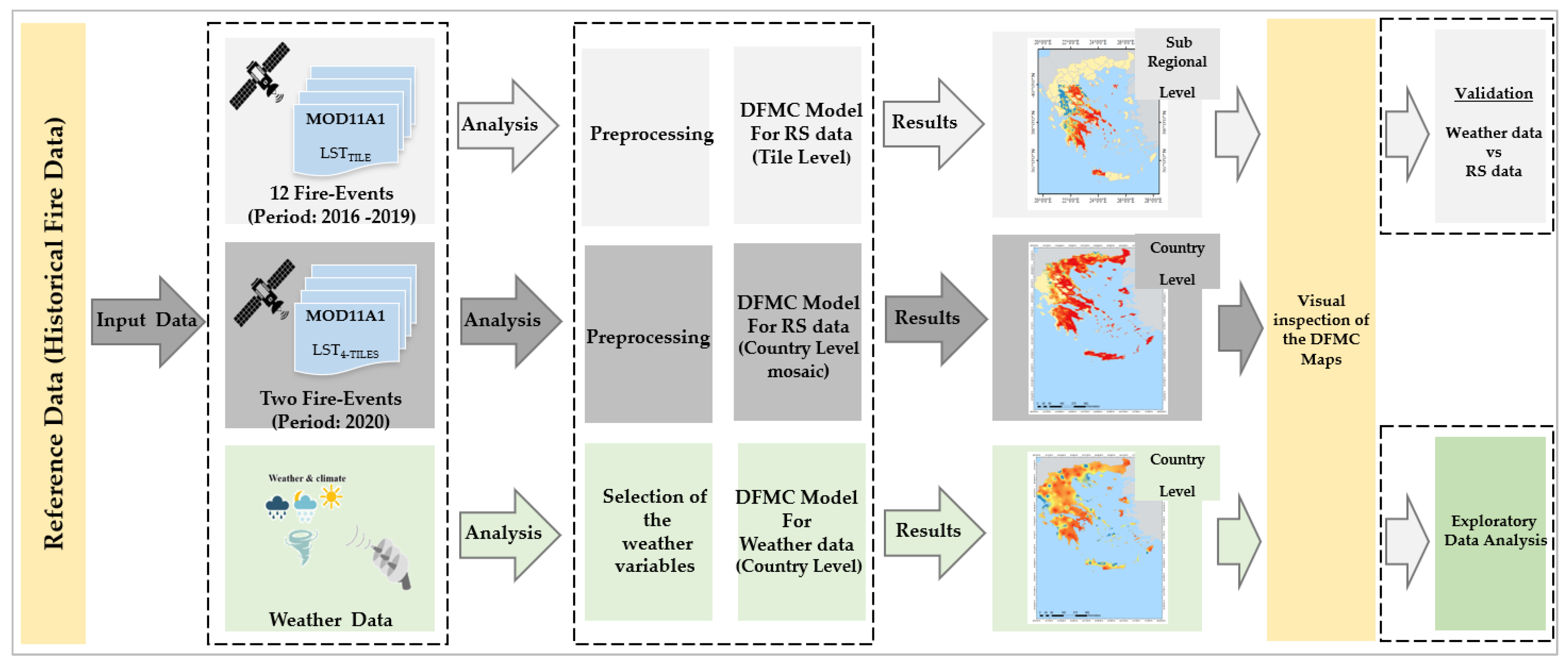
2. Materials and Methods
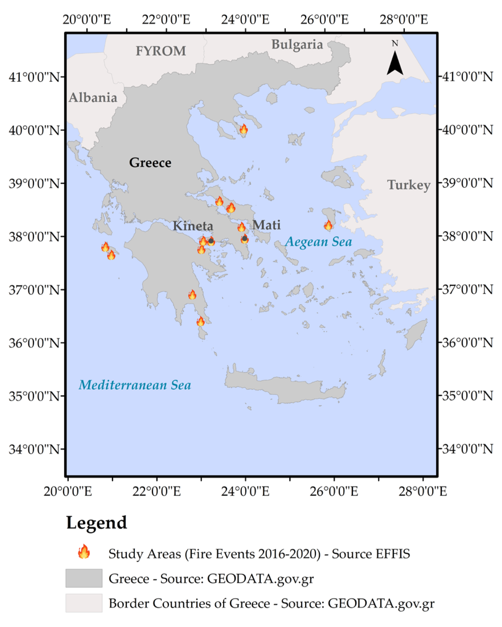
The present study evaluates the model proposed by Nolan et al. [35,46] in terms of estimating DFMC during severe fire events in Greece. An outline of the applied methodology is presented in Figure 1. Historical fire data, weather records and satellite data were used during this study in order to estimate DFMC at various spatial scales in Greece. After preprocessing, the MODIS data and the meteorological data were separately analyzed to estimate DFMC, using Nolan’s proposed approaches. The implementation of the two different approaches, namely, MODIS DFMC model and the AWSs DFMC model, resulted in several DFMC maps, at various spatial scales. The production of the DFMC thematic maps was followed by the process of validation. Unfortunately, due to a lack of DFMC field measurements, the validation process was feasible only in the case of the mapping products that have been derived from the satellite data. Hence, the next process that took place after the implementation of the Nolan’s proposed approaches was the validation of the MODIS DFMC thematic maps. The derived thematic maps at sub-regional level were validated using daily surface station observations. During the validation process the daily surface station observations were used as ground truth data. More specifically, for each examined day and AWS station the two variables, D and DFMC, were estimated at point level. Next, the derived variables were used to validate the mapping products that have been derived from the MODIS DFMC model. Subsequently, for each examined date, the estimated MODIS-based values were compared against the AWSs derived variables (point level), using selected statistical measures.
The validation process was supplemented by thorough visual examination of all of the thematic maps (MODIS DFMC and AWS DFMC maps) produced during the implementation stage. In the end, an exploratory data analysis was conducted in order to understand how the specific models perform in Greece. All of the analyses have been carried out using the free and open-source software R. The rest of this section describes the datasets used and the various parts of the methodology.

2.1. Study Areas

The proposed methodology has been tested using historical fire data from fourteen (14) wildfires in Greece (Figure 2 and Table 1). The examination period spanned from 2016 to August 2020. The considered fire events were selected to cover representative cases from different environments in Greece. In the case of the MODIS DFMC model, the analysis was conducted in two spatial scales regional and national. After the implementation of the DFMC model at regional scale we produced sub-regional DFMC thematic maps by using the limits of the areas of interest (Figure 1). The reason for initially applying the MODIS DFMC model at regional scale is because before applying the specific model at national scale we wanted to evaluate the use of this approach in representative Greek ecosystems. Additionally, in the case of the AWSs DFMC model the analysis was conducted only at national level, due to the fact that in some cases the number of the AWSs stations was not appropriate for sub-regional DFMC mapping. For the purposes of the analysis, we selected the areas located in Kineta and Mati, in Attica, as pilot sites. These areas were affected by large and devastating fires in July 2018. The fire in Mati was the deadliest fire in Greek history and the second-deadliest weather-related disaster in Greece, the major heat wave of July 1987 being the deadliest [57].
In this study, two approaches were used for estimating DFMC. The first approach utilized daily MODIS LST products (MOD11A1) [58] with approximately 1 km × 1 km spatial resolution, while the second one utilized meteorological data recorded at 10-min intervals [59]. During the implementation of the first approach (MODIS DFMC model), twelve out of the fourteen fire events (Set 1) were used during the analysis at regional and sub-regional level (Set 1), while the remaining two were used in the analysis at country level (Set 2) (Table 1). At this point, it should be clarified that the DFMC in the case of the fire events, which were carried out in the pilot areas, was estimated both at regional and national level. As was previously mentioned, the sub-regional DFMC maps were derivatives of the regional DFMC maps. The justification for applying the MODIS DFMC model at regional level is that the specific model is primarily designed for this type of spatial scale. As for the second approach (AWSs DFMC model), we chose to apply the proposed methods in the fourteen historical events (Set 1), which were also used in the analysis of the first approach at national level. At this point it should be mentioned that apart from one fire case (Sarti’s fire, see Table 1), all the other wildfires took place during the summer season (dry conditions). The exception in the fire cases of this study is the Sarti’s fire that took place in the end of the fire season, and more specifically in October (humid conditions). Usually at this time of season, the weather conditions are wet and humid, and thus not favorable for fire spread. The weather data from the meteorological station closest to the Sarti’s fire affected area show that during October the weather conditions were anomalously dry, with only 1.6 mm of rain recorded. The peculiar conditions prevailing in the region of Sarti’s fire constitutes the specific fire incident a special case in this study.

2.2. Reference Datasets

To assist the process of the analysis we used the official fire perimeters of selected dates (see Table 1) along with information for the ignition points. The first dataset was provided by the EFFIS European database, while the second one was provided by the Hellenic Fire Corps. The two datasets were used to match the fire locations and dates with the satellite data that we would like to acquire for the analysis.
In addition to the two aforementioned datasets, the Advanced Spaceborne Thermal Emission and Reflection Radiometer (ASTER) Global Digital Elevation Model (GDEM) (https://asterweb.jpl.nasa.gov/gdem.asp, accessed on 20 May 2020) (30 m) and the 2018 version of the CORINE Land Cover (https://land.copernicus.eu/pan-european/corine-land-cover/clc2018, accessed on 22 May 2020), were also considered during the analysis.

2.3. Satellite Imagery

To estimate DFMC on a daily basis, we used the MOD11A1 Version 6 product from the MODIS sensor on Terra satellite. MOD11A1 provides observations of daily Land Surface Temperature (LST) and Emissivity (E) values at 1km spatial resolution. The C6 MODIS 1-km LST product is provided projected in a Sinusoidal grid and cloud-free, along with night and day LST values, quality flag indicators, emissivity values, view zenith angles and time of observations. The LST products (Table 2) used in this study were downloaded directly from the Application for Extracting and Exploring Analysis Ready Samples (AppEEARS) (https://lpdaacsvc.cr.usgs.gov/appeears/, accessed on 5 June 2020). In the current study, this was conducted manually although it is in our future intentions to automate this step. As mentioned in a previous paragraph, MODIS LST images were acquired before, during and after the fire events (Set 1 and 2). The pre-fire date was set a day prior the wildfire event and the post-fire date a day after the event.
At this point, it is important to note that the methodology was initially applied on selected MODIS tiles (1200 km × 1200 km), which coincided with concrete fire events. The selection of the aforementioned tiles was based on trustworthy information regarding selected fire ignition locations (please refer to Table 1). Henceforth, each MODIS tile, which corresponds to one date, will be referred to as LSTTILE. Subsequently, the MODIS DFMC model was applied to a larger area, namely, Greece. To cover the Greek area with satellite data, four MODIS tiles in HDF format (LST4-TILES) were acquired for predefined dates (please refer to Table 1 and Table 2). In this case, the dataset which corresponds to four MODIS tiles per date will be referred to as LST4-TILES.
For data processing purposes, the MODIS images (LSTTILE per date) were reprojected from the Sinusoidal to WGS84 Geographic projection. Subsequently, as indicated in Nolan’s et al. [46] study, the images were corrected to avoid data anomalies (viewing zenith angles > N 50.5°). More specifically, the contaminated pixels were masked out from the reprojected MODIS products using the quality assurance (QA) information. Ultimately, based on the QA metadata, the daily LST data with the highest-quality (quality control flags set to 00) were selected for the analysis [46,48].
In the case of the LST4-TILES MODIS datasets, we followed the same analysis steps except from the part that we had to mosaic the image products. At this point it is important to remind the reader that the LST4-TILES MODIS datasets were downloaded and utilized in two out of the fourteen historical events (Set 2) and in the pilot area, which is located in Attica, Greece.
Regarding the level of analysis, it should be stressed that we initially chose to apply the MODIS DFMC model at sub-regional level, because the specific model is designed to be applied, preferably, in this type of scale. After the evaluation of the DFMC model at several Greek ecosystems we applied the model at the national level in order to investigate the quality of the MODIS DFMC maps in this type of scale. The MODIS DFMC model at national level was applied during the dates that the wildfires at Mati, Kechries and Lagada (Table 2) took place. The MODIS DFMC model was carried out at national level because we wanted to compare the quality of the MODIS DFMC maps against the quality of the AWSs DFMC maps. The selection of the two fires for the fulfillment of this task, at Kechries and Lagada, was based on the fact that, for both fire events, it was not feasible to acquire pre-fire MODIS data.

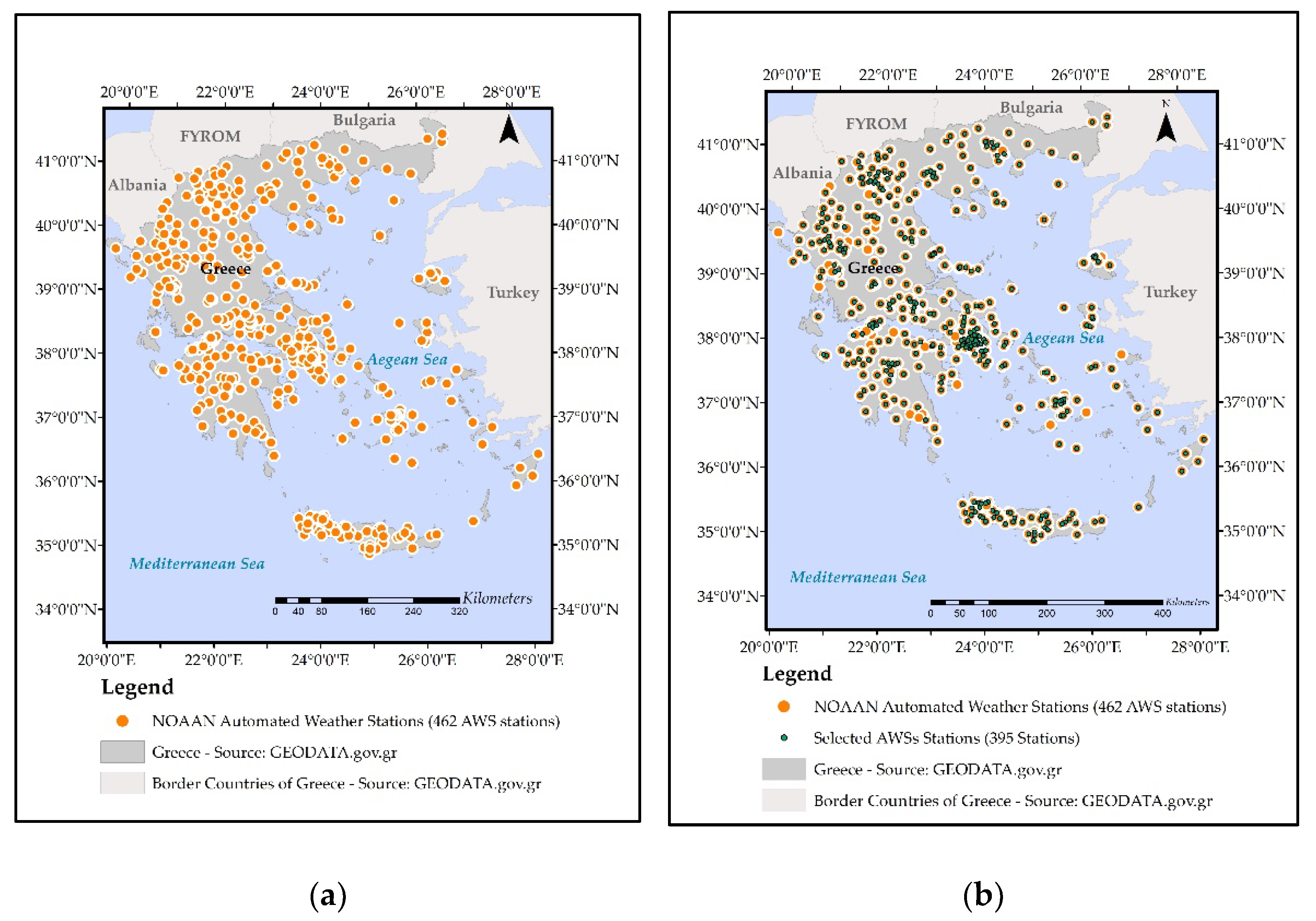
2.4. Meteorological Data

Meteorological data were obtained from the dense network of automatic weather stations (AWSs) operated by the METEO unit at the NOA (NOANN, http://meteosearch.meteo.gr, accessed on 10 June 2020) [59]. The NOAAN is the denser network of weather stations in Greece (462 stations in 2021) (Figure 3a), which has been specifically designed to cover the whole territory of the country [59]. Regarding the position of the AWSs in the Greek territory, it is important to note that several of the stations are located in agricultural and suburban areas and their elevation ranges between 2 to 2240m. The weather data are recorded in 10 min intervals and they are stored in an advanced database at NOA premises [59]. The data selected for this work were exported from the NOA’s database in the form of tab-delimited text files. The acquisition dates of the weather data correspond to the dates presented in Table 1 (Set 1).
For the current analysis, data from 395 out of the 462 AWSs have been used (Figure 4a,b). The selection of stations was limited to those that were more than 2 kilometers apart (2 MODIS pixels) and they were not located in port areas. The dataset resulted from the selection process was used during the implementation of the DFMC equation based on meteorological data. More specifically, the selected AWSs were used during the interpolation phase in order to map the weather variable D and subsequently DFMC. Ultimately, the AWSs were used during the validation process as ground truth data (see Section 2.5). To clarify that, for each examined date, the daily meteorological data (point data) from the AWSs were used for the estimation of the two variables, D and DFMC at point level. The variables derived from this process served as ground truth for the validation of the mapping products that were derived for each different fire event.

2.5. Dead Fine Fuel Moisture Content—DFMC

The main objective of this study is to map the DFMC of the study areas on predetermined dates (Table 1) by using separately MOD11A1 LST products and weather observations. To this end, we have selected to test the spatial application of the Nolan’s recently developed DFMC model [46]. This method’s main advantage is that the DFMC can be estimated and monitored using a simple model without the need for site specific calibrations. The proposed model is based on a robust theoretical framework [35,46] and its use was adopted due to its high capacity for operational DFMC mapping and monitoring [11].
The specific model is based on the notion that DFMC increases when D decreases. Based on this notion, daily variations in the DFMC can be reliably calculated and mapped from gridded D estimates [11]. D can be in turn estimated either from satellite data or from weather observations. To link all the essential variables for the estimation of the fuel moisture content Resco de dios et al. [35] proposed the following Equation (1):
FM = FM0 + FM1e(−mD)
where FM is the minimum FM, FM0 the minimum fuel moisture content (%), FM0 + FM1 is the FM when D is zero, and m is the rate of change in FM with D (kPa). In the recent past, Nolan et al. [46] calibrated and validated this model in order to propose new values for the parameters FM, FM0, and m. At this point it is important to note that the specific parameters vary, depending on whether we use satellite or meteorological data. Table 3 details the model parameters proposed by Nolan et al. [46] for each different case. According to Nolan et al. [46], the concrete parameters have been tested and validated in various types of vegetation [31]. For more details about the model adopted in this current study, the readers who are interested may refer to the cited references.
During the experimental analysis, three different datasets were used as inputs in the model, namely, the LSTTILE, LST4-TILES and the daily meteorological dataset. To fulfill the requirements of the first approach (MODIS DFMC model), the proposed model was applied to large wildfires in Greece. For each examined fire event the two variables, D and DFMC, were estimated on a daily basis before, during and after the event, at sub-regional level, using the LSTTILE datasets (Set 1) (see Table 1 and Table 2). D was estimated based on the empirical relationship proposed by Hashimoto et al. [48]. After the completion of the previous stage, the same variables, D and DFMC were estimated at national level, by using the LST4-TILES datasets (Set 2) (see Table 1 and Table 2).
Afterwards, the two aforementioned variables were estimated again, this time using data from automated weather stations. The estimations were repeated for a series of dates that correspond to the fourteen fire events (Set 2) (see Table 1). Before the implementation of the AWSs DFMC model, for each examined date, daily D was calculated through spatial interpolation of data from the selected AWSs. The spatial interpolation technique applied in this study is the ordinary kriging [60]. The same technique has been also applied in a similar application by Hashimoto et al. [48]. At this point, it should be noted that the number of stations used in the interpolation procedures, varies about 10% from day to day due to eventual temporary disruption and partial loss of data. The previously mentioned DFMC estimations were performed at national level.
The application of the previously mentioned model on each daily dataset (LSTTILE, LST4-TILES, or daily meteorological observations) resulted in two thematic maps. The first map depicts the modelled vapor pressure deficit (D), whereas the second map depicts the modelled DFMC. At this point it is important to clarify the spatial extent of each mapping product. The thematic maps derived from each different LSTTILE, per date, depict the calculated variables on tile level. The same variables (D and DFMC) were produced at a larger scale at country level for Greece, when the LST4-TILES and the daily meteorological datasets were used, respectively. The resulting DFMC maps were subjected to visual examination.
At the methodology’s final stage, the thematic maps derived at sub-regional level were validated using daily meteorological data observations.

2.6. Exploratory Data Analysis

To investigate the way the two equations (models) proposed by Nolan et al. [46] behave under the same circumstances, an exploratory data analysis was conducted. Hence, a dataset of theoretical D values was created. The dataset range was between 0.05 and 7 kPa, while the data step to create the new set of values was set to 0.025 kPa (theoretical values). The range of the values was selected based on the range of the D values given by the MODIS-based and AWS-based equations. Subsequently, the same dataset of D values was used to calculate DFMC from both equations (models). Finally, the spatial distribution, of the deviations between the MODIS-based DFMC and the AWS-based DFMC (MODIS DFMC -AWS DFMC), was visualized.

2.7. Validation Process

Due to a lack of DFMC field measurements, the validation of the produced maps was possible only in the case of the thematic maps that have been derived from the satellite data. Emphasis was given on the validation of the derived thematic maps, on a tile level. To this end, all of the tile level maps were validated by using surface weather observations. The validation process was supplemented by thorough visual examination of the thematic maps produced during the implementation stage. Specifically, for individual LSTTILE based thematic map the fire affected areas were isolated and visually inspected. For each different fire date (before, during and after the fire event) the pixels with the highest daily DFMC were located and examined regarding their position within the area of interest.
A necessary step before the validation process was to remove spatial heterogeneity from the satellite variables derived from the LST MODIS products. For this reason, each of the MODIS derived variables was averaged using a 3x3 window and centered over each of the AWSs location [46]. For each examined date, the estimated, MODIS-based values were compared against the AWS derived variables, using selected statistical measures, namely, the Root Mean Square Error (RMSE), the mean absolute error (MAE) and the mean biased error (MBE). Henceforth, the estimates (point data) from the MODIS based model will be referred as MODIS D and MODIS DFMC, whereas the weather-station based estimates (point data) will be referred to as AWSs D and AWSs DFMC, respectively.
Furthermore, to proceed to a more thorough investigation of the results, scatterplots and Kernel Density Estimation (KDE) plots were employed for each fire event separately as well as for the whole set of data.

3. Results

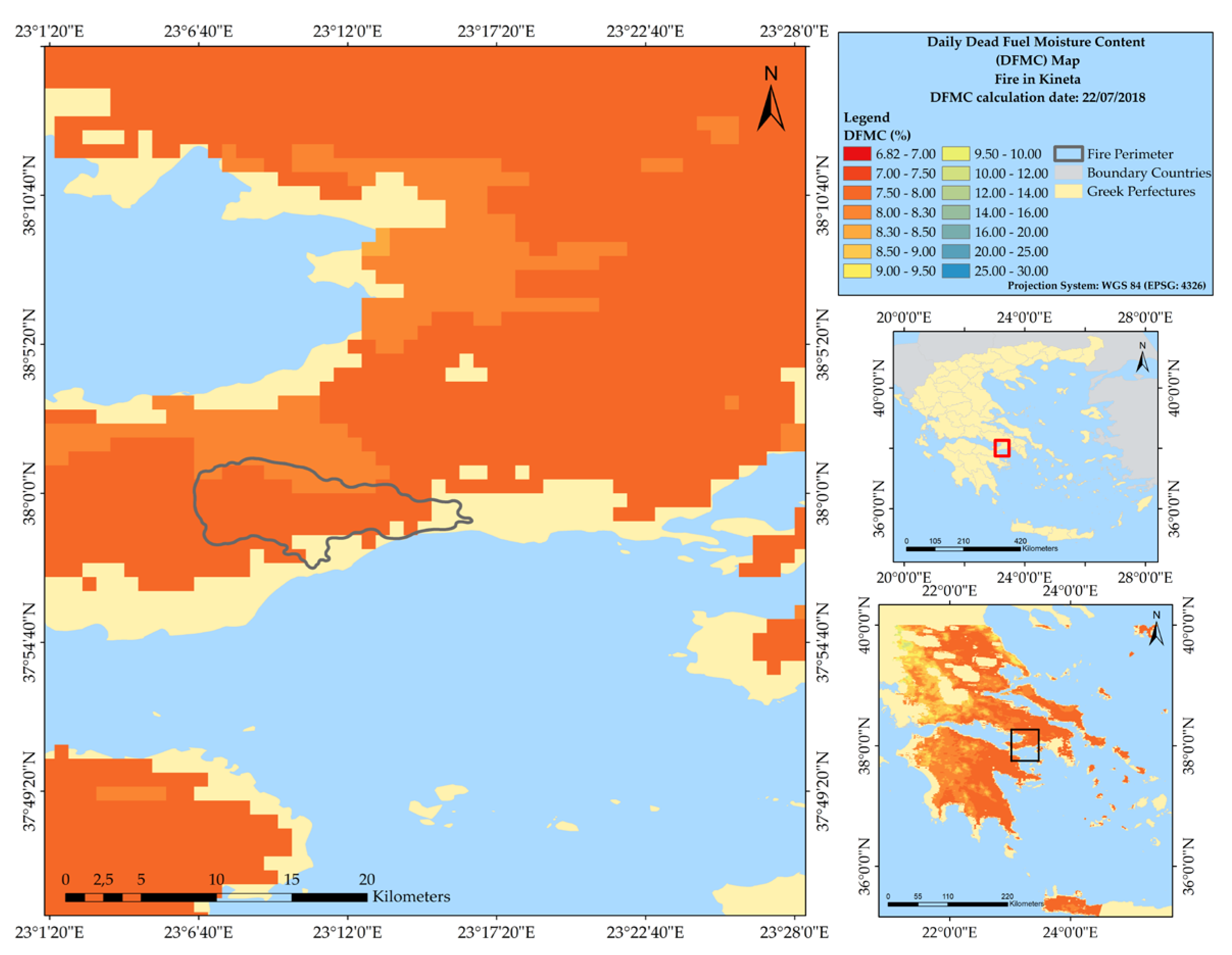
3.1. Satellite-Based DFMC Maps

In this section, the mapping products derived from the MODIS DFMC model are initially presented. The thematic maps, derived from LSTTILE and LST4-TILES datasets, are presented in Figure 4, Figure 5 and Figure 6. Due to the large volume of results, we will only present the results obtained from the study of the pilot areas at Kineta (Figure 4 and Figure 5) and Mati (Figure 4 and Figure 6). At this point, it should be stressed that the previously mentioned wildfires started on the same date (23 July 2018) and coincide in the same MODIS LST tile.
Figure 4 illustrates the different limits of the derived MODIS DFMC maps after the implementation of the MODIS DFMC model at various scales. Particularly, the sub-regional thematic map in Figure 4a presents an example of the limits of the tile-based DFMC map. In order to facilitate the comparison between the limits of the different maps Figure 4b presents the DFMC map produced at a country level. The first Figure in this section (Figure 4) illustrates the way that the DFMC values vary on a daily basis at sub-regional and national level. The date of the two MODIS DFMC maps of Greece is the 22 July 2018, a day prior to the catastrophic fires at Kineta and Mati. Additionally, Figure 5 presents the way that DFMC varies a day prior to the wildfire at Kineta region. Next, Figure 6 presents the DFMC dynamics before, during and after the fire event at Mati.
Our analysis of historical fire events indicates that in all cases, the fire events took place under extreme fine fuel dryness. In all examined cases (12 wildfires), the maximum DFMC values attained inside the fire perimeters were well below the flammability thresholds indicated in the literature (~12–14%) [11,29]. More specifically, in all of the cases that were examined, apart from 1, the DFMC values inside the fire perimeters did not exceed 9.1% during any of the examined periods. Only in the case of Sarti’s fire at Chalkidiki, the DFMC values amounted to 15.08%. Subsequently, a closer examination of the MODIS DFMC maps revealed that, inside the fire perimeters, the pixels with the highest DFMC values are usually located in areas close to the sea and consequently belong to wildfires that took place near the shoreline.
To assist the evaluation of the MODIS DFMC maps, a visual examination of the results was also carried out. The findings of the examination indicate that the gaps in the MOD11A1 LST products, which are mainly caused by the presence of clouds and wildfire smoke, affect the maps’ quality [46]. Figure 6c,d illustrate an example of the non-feasibility of estimating the DFMC inside the fire perimeter (the fire at Mati) due to the image gaps. In addition, the removal of the pixels with viewing zenith angles >50.5° during the preprocessing stage resulted in the deterioration of the data gap problem. Nevertheless, in all of the examined cases the majority of the bad quality pixels have been removed by the provider.

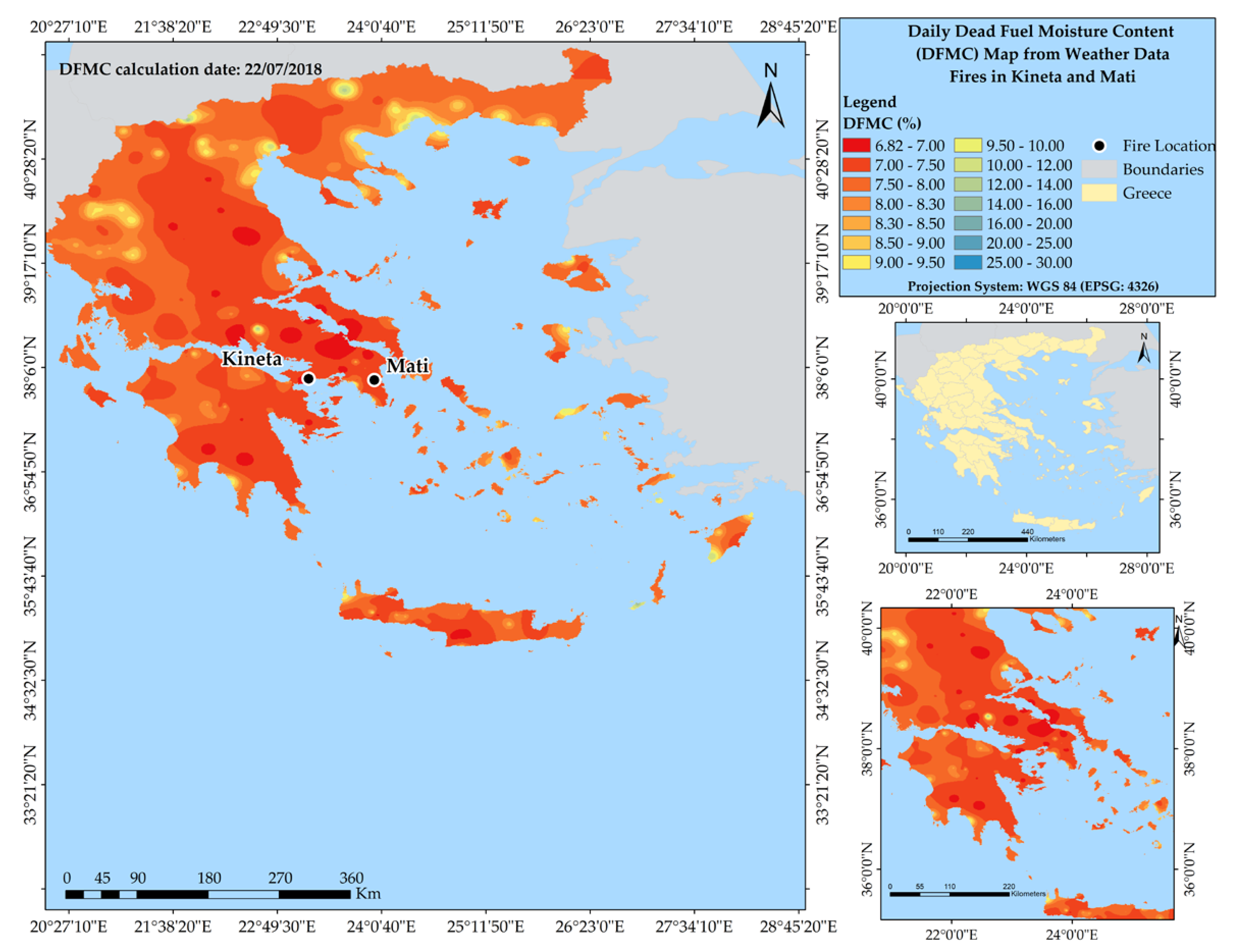
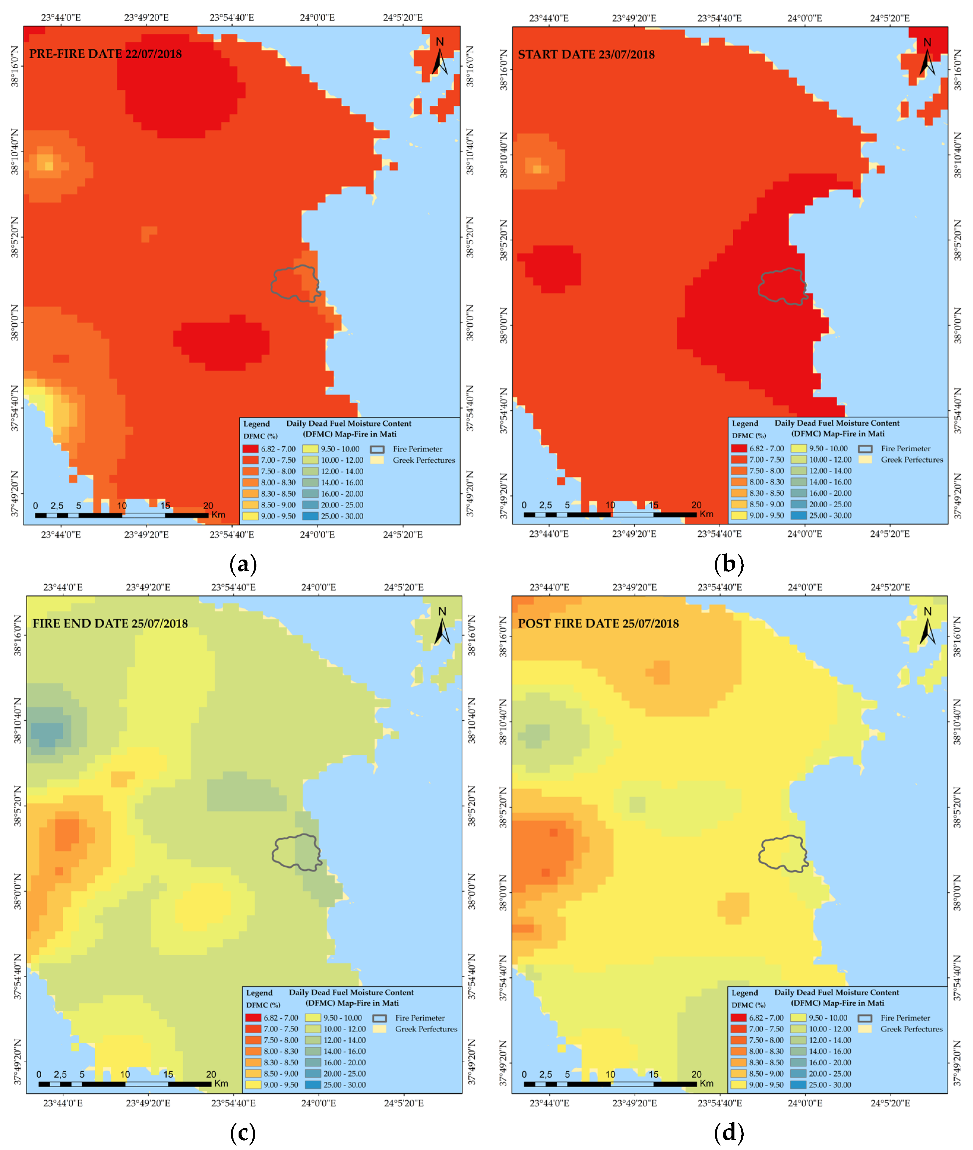
3.2. Weather Station-Based DFMC Maps

The results obtained by applying the AWSs DFMC model (weather-station based DFMC model) are presented in Figure 7 and Figure 8. Figure 7 presents the DFMC map produced at a national level, using ΝOAΝΝ stations, on the 22 July 2018, a day prior to the fires at Kineta and Mati (Attica Region, Greece). Subsequently, Figure 8 presents the DFMC maps for the period from 22July until 25 July 2018.
The analysis of the values of DFMC in the produced maps indicated similar results to the previous approach (see Section 3.1). Similarly to the AWSs DFMC model and in relation to all of the cases examined, Sartis’ fire case was the one that stood out due to the higher observed DFMC values (DFMC reached up to 19.23%) inside the fire perimeter, during the dates we examined. As mentioned in a previous (Section 2.1) Sarti’s fire is a special case. The reason for that is because the fire incident took place in October at the end of the fire season and not during the dry period of the year. Another reason that constitutes the Sarti’s fire incident a special case is the fact that the examination of the weather statistics showed that the specific area received very little precipitation during the traditionally wet month of October. The results presented above confirm the fact that the Sarti’s fire is an exception and should be further examined. Moreover, the numerical results obtained by the AWSs DFMC model also indicate that in all the cases examined, the DFMC values inside the fire perimeters were slightly higher compared to the satellite-data based DFMC values. Examination and visual interpretation of the derived maps from both approaches suggest that the AWSs DFMC maps show higher spatial continuity in comparison to that derived from the MODIS-based approach. This is attributed to the gap problem in the satellite images, which inevitably leads to the production of incomplete maps. At this point it should be noted that the quality of the AWSs DFMC maps was only assessed visually due to a lack of DFMC field measurements. To explain that, the AWSs DFMC model was only assessed for its ability to produce complete products (spatial continuous DFMC maps). The validity of the derived AWSs DFMC maps were only examined locally, in specific regions, by experts who were familiar with the local vegetation and weather conditions.

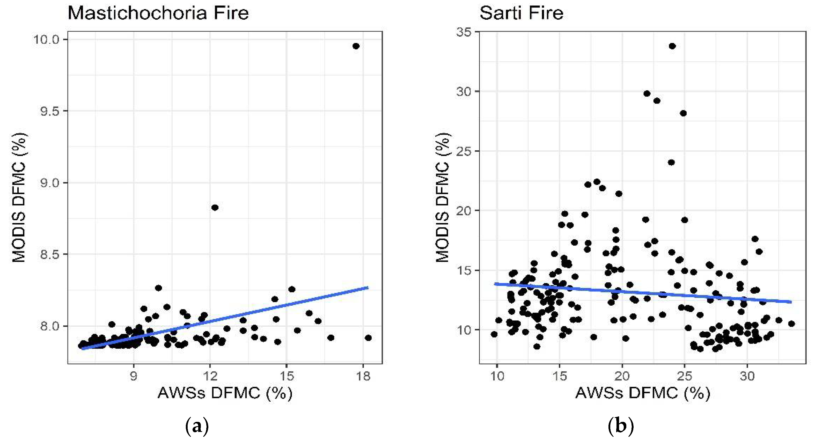
3.3. Validation and Exploratory Data Analysis Results

3.3.1. Exploratory Data Analysis Results

In order to investigate the way that the two approaches, namely the MODIS DFMC model (satellite-based) and the AWSs DFMC model (weather-station based), proposed by Nolan work in practice, an exploratory data analysis was performed. At this point it is important to remind the reader that the values used during this analysis are theoretical (see Section 2.7). The results of this process indicated that for extremely low values of D < ~0.6 kPa (water vapor saturated atmosphere, humid conditions) the MODIS DFMC model results in increased DFMC, compared to the AWSs DFMC. In addition to that, in the range between 1 to 3 kPa (D values), the MODIS DFMC model results in decreased DFMC compared to the AWSs data DFMC. For D values > 3 kPa (the atmosphere starts to dry out) the MODIS DFMC model ceases to respond (the exponential decrease in DFMC stops), in contrast to the AWS DFMC model which continues to provide exponentially decreasing values of DFMC. Hence, for D values > 3 kPa the MODIS DFMC model continues to result in higher DFMC values, in comparison to that derived from the AWS DFMC model.
The scatterplots and the KDE plots, produced between the variables MODIS D and the AWSs D, revealed that the equation, which was used to estimate D from MODIS data equation, underestimates D (not shown). This finding means that the MODIS data produce biased estimates of D under dry conditions.

3.3.2. Validation of the Satellite—Based Variable Water Vapour-Pressure Deficit D

The accuracy of the MODIS D variable values, against the respective variable derived from the AWSs ground observations (AWSs D) was assessed by calculating three statistical metrics, namely, the MAE, the MBE and the RMSE. Table 4 reports the numerical results from the calculations. An examination of the obtained results showed that in all cases examined, apart from one (Sarti wildfire tile, ΜΒΕ (0.14 kPa), the MODIS D tended to underestimate the AWSs D, with MBE ranging from −0.22 kPa to −1.19 kPa. The lowest MBE (−1.19 kPa) was observed in the MODIS tile, which coincides with the wildfire at Elafonissos, while the highest MBE was observed in the tile, which coincides with the wildfire at Sarti (0.14 kPa). In all of the examined cases, apart from Sarti’s fire case, the low values of MBEs indicate that the MOD11A1 satellite data underestimate D in areas where, according to AWSs, the conditions are dry. In addition, the comparison between the satellite- based and the AWSs D resulted in RMSEs ranging from 0.62 kPa to 1.54 kPa, and MAEs ranging from 0.52 kPa to 1.26 kPa. A higher difference between the two metrics (RMSE − MAE = 0.37 kPa) was observed in the case of the tile, which coincides with the wildfires at Kineta and Mati (MAE = 1.16 kPa). The calculated differences between the RMSE and the MAE resulted in low values in all cases. This finding indicates that the variation in the values of the individual errors is small.
The relationship between MODIS D and AWSs D was further examined by using scatterplots (not shown). Visual exploration of the resulting plots revealed that in all cases examined, apart from Sarti’s fire case, there is a positive but weak relationship between the two variables. In the case of Sarti’s fire the scatterplot (not shown) indicates that correlation between the MODIS D and AWSs D is negative but very weak. The main reason for that is the fact that according to the CORINE 2018 dataset, the majority of the AWSs are located in areas covered by complex cultivation patterns or discontinuous urban fabric areas. In general, the region contained in that specific MODIS tile is characterized by high heterogeneity. Even though the AWSs show the real values of the D variable, the sample of the AWSs used in the validation does not cover the heterogeneity of the area.

3.3.3. Validation of the Satellite-Based DFMC

This section presents the results obtained from the comparison of MODIS DFMC and AWSs DFMC. The obtained numerical results (Table 5) indicated that in all of the examined cases, the MODIS DFMC model tended to underestimate DFMC, with MBE ranging from −0.29% to −7.29% (Table 5). The results among the different examined cases indicated that the case with the highest MBE value (−7.29%) and, consequently, the one with the highest underestimation was the Sarti’s fire case (tile level). In addition to that, the results illustrated in Table 5, show that the RMSE values observed in the validation datasets range from 1.63% to 10.99% and the highest RMSE error (10.99%) is observed, again, in the case of Sarti’s tile (MAE:8.23%). Contrary to that, the lowest RMSE error (1.63%) was observed in the tile which coincides with the fire at Elafonissos (MAE 0.97%). At this point, it is worth mentioning that Sarti’s fire is the only fire incident which occurred in the northern part of Greece in the middle of the autumn period (October). At this time of the season, dry and cold conditions usually prevail in this part of Greece. According to the Köppen’s climate classification map, the specific region is categorized into the regions with cold semi-arid climate. However, as it was previously mentioned in Section 2.1, the weather conditions in October 2018 were abnormally dry. The majority of the other fire incidents occurred in the southern part of Greece, during the summer period (July and August). The climatic conditions in this part of Greece are significantly drier and hotter compared to the conditions in the northern region, particularly at the end of the autumn season.
Complementary to the numerical results reported above, the two variables’ scatterplots, MODIS DFMC and AWSs DFMC, for each different fire case were also created (not shown). The visual exploration and ability to interactively select elements from the scatterplots proved very useful in this study in providing valuable findings. In all of the cases examined, apart from the Mastichochoria and Sarti fires, the visual exploration of the scatterplots revealed that the relationship between the variables MODIS DFMC and AWSs DFMC is positive but relatively weak. Specifically, the visual examination of the scatterplots revealed that the relationship between MODIS DFMC and AWSs DFMC shows a stronger correlation in the Mastichochoria’s fire case, whereas in the Sartis’s fire case it shows a weaker correlation. Figure 9 presents the two scatterplots for the two fire cases. Furthermore, the study of the scatterplots in the fire cases of Kineta-Mati (one case) (not shown) and Kalamos (second case) (not shown) showed that, after a point, the MODIS DFMC model resulted in increased DFMC compared to the DFMC, which resulted from the AWSs model. This finding applies to all of the cases examined. The explanation for the MODIS DFMC model specific behavior can be found in the exploratory analysis results. More specifically, according to the exploratory analysis results, when the observed D is extremely low (D < ~0.6 kPa, moist conditions) then the MODIS DFMC model results in increased DFMC, compared to the AWSs DFMC. Moreover, when the observed D is greater than ~3 kPa (the atmosphere starts to dry out) then the MODIS DFMC model ceases to respond (the exponential decrease in DFMC stops), in contrast to the AWS DFMC model which continues to provide exponentially decreasing values of DFMC. Thus, for D values > 3 kPa the MODIS DFMC model continues to result in higher DFMC values, in comparison to that derived from the AWS DFMC model. Therefore, according to the above, when the conditions are dry the MODIS data shows low capability in estimating DFMC. Apart from the previous mentioned graphs, scatterplots and KDE plots were also created for the examination of all the fire cases together (Figure 10). The visual inspection of the plots (Figure 10) revealed that the higher the estimated AWS DFMC, (moist conditions) the greater the underestimation of the MODIS DFMC. In many cases the DMFC underestimation reaches up to 20% (Figure 10). This is partly attributed to the location of the AWSs and to the problematic performance of the DFMC model under wet conditions [46]. Ultimately, the representation of the spatial distribution of the differences between MODIS and AWS DFMC revealed that there is a concentration of large deviations in the northern part of Greece associated with the Sarti’s fire. As previously mentioned, these deviations observed in AWSs are mainly located inside areas covered by complex cultivation patterns and in discontinuous urban fabric areas. In the remaining part of the Greek country (the northern part is excluded), the AWSs with the larger deviations are located at Karpenisi (land principally occupied by agriculture), Tyria (land principally occupied by agriculture), Vovousa (sparsely vegetated area), Parnassos (sparsely vegetated area), Pertouli (discontinuous urban fabric) and in small islands. The specific stations exhibit some common site characteristics. More specifically, the stations are located in high altitude regions and humid environments. In addition to that, the measured precipitation values at the individual stations are significantly higher in comparison to that obtained from the other stations.

4. Discussion

4.1. Performance of the DFMC Model

The experimental results in all of the examined cases revealed that the wildfires took place under very flammable conditions. More specifically, in the majority of the analyzed fire cases, the estimated DFMC inside the fire perimeters did not exceed 14% (Table 6). Only in the Sarti’s fire case did we observe that the DFMC which resulted from both approaches (MODIS DFMC = 15.08% and AWSs DFMC = 19.23%), exceeded the limit of 14%. The findings of this research are consistent with previous studies [2,11,61] that found similar DFMC thresholds of flammability. The fact that the implementation of Nolan’s model, by using two approaches, results in similar flammability thresholds with other studies, suggests that the DFMC model based on the estimation of the water vapor pressure deficit (D) can be used for the estimation of the critical flammability thresholds, at regional or national level, in Greece.
In areas where the weather conditions were dry, the results from the exploratory analysis indicated that the equation based on the MODIS data did not satisfy estimate the variable D. This finding was also confirmed during the validation of the variable, and it is consistent with similar findings in previous studies [46,48]. Specifically, according to Hashimoto et al. [48] and Nolan et al. [46], the calculation of the D variable is problematic in arid and low vegetation areas (LAI < 0.5). The previously mentioned studies have reached the conclusion that the calculation of D from MODIS data is more preferable in areas with high vegetation cover (LAI > 0.5) [46]. At this point, it is important to mention another important finding of this study. Poor estimation of D was observed not only in arid regions but also in semi-arid regions. More specifically, poor estimation of D was mainly found in the northern part of Greece, where the climate is characterized as cold semi-arid. The area where the Sarti’s fire took place is also located in the cold semi-arid zone. The findings regarding the estimation of the D variable in arid regions and semi-arid regions are consistent with the findings from previous studies [46,47]. D’s poor estimation can be explained by the fact that the LST, retrieved by MODIS data, depends on the accuracy of the surface emissivity [62]. The LST MODIS data measurements may contain large errors and uncertainties in arid and semi-arid regions, where the surface emissivity shows high spatial and temporal variations [62].
In our study the sites where the MODIS data failed to accurately, estimate D are agricultural areas characterized by complex cultivation patterns (irrigated areas, non-irrigated areas, olive plantations, discontinuous urban fabric areas etc.) At this point it should be mentioned that the validation of the AWSs derived D was not possible due to a lack of field measurements and consequently it was not possible to compare the two different products. Apart from the above, the use of different equations in calculating D may have affected the results. More specifically, MODIS D was calculated based on TLST (land surface temperature) using the equations proposed by Hashimoto et al. [46], while the AWSs D was calculated based on the daily maximum Tair (land surface temperature). The two equations have utilized very different variables and to this end the deviations in the results were expected.
The results obtained from the validation of MODIS DFMC indicated that in all cases examined, apart from one, the performance of the MODIS DFMC model was similar to previous studies [35,46]. More specifically, the MAE of DFMC in our study was less than 2.2%, when MODIS DFMC was compared against AWSs DFMC, whereas the reported DFMC MAE in the literature is less than 2.9% [46]. The case with the most problematic MAE was the Sarti’s fire case. The MAE in that case reached up to 8.23%. So, according to the above, the performance of the MODIS DFMC model at regional level in Greece was acceptable apart from one.
In addition, in all of the examined cases (Sarti’s fire case included), the results showed that the MODIS DFMC model resulted in underestimated DFMC. The results showed that the higher underestimation of the DFMC was observed on AWSs, where the weather conditions were humid. The fact that the performance of the MODIS DFMC model may be poor under moist conditions has already been reported in previous studies [46,63]. According to the literature, dead FMC is significantly variable under wet conditions [63]. Consequently, the presence of high variability at higher moisture contents in the validation statistics obscures the information about the model’s performance in the cases where fuel will burn. According to Nolan et al. [46], this fact does not limit the operational capability of the model, because any dysfunctionality in the model’s performance is observed when the moisture content in the dead fuels is greater than 30% (non-flammable conditions). In addition to that, it is worth mentioning that the physical processes that govern DFMC in forests are very complex, and under a specific range of conditions the DFMC models are failing to correctly estimate the moisture content of the dead fuels [63]. In previous studies [48,63] it has been reported that when the conditions are too wet or too dry the DFMC models exhibit low performance. Apart from the above, in our specific study, the underestimation of DFMC is partly explained by the occurrence of sea breezes in the coastline. The presence of sea breezes in a region means that there is a water advection onto land, a fact that leads to the overestimation D and subsequently to the underestimation of DFMC. Greece’s coastline is the longest in the Mediterranean area and the 11th largest in the world. Hence, the weather of a significant part of the country that is located near the coastline is usually affected by the sea breezes. However, as it was stated before, the occurrence of the sea breezes in the study areas partly explains the overestimation of D and thus the underestimation of DFMC. This finding has already been reported by Hashimoto et al. [48] and needs to be further investigated in our future studies. At this point it is important to note that every year most of the Greek fires are occurring in forested areas that are located close to the coastline. In this specific study most of the fires are located in areas relatively close to the coastline (Figure 1). The fact that the results in the Sarti’s case showed poor model performance may be attributed to the fact that the validation process was conducted in irrigated and non-irrigated agricultural sites, where the moisture conditions vary to a significant extent. Another reason that can be attributed to the model’s poor performance during the Sarti case is the fact that the specific fire occurred during the middle of the autumn season and at the end of the fire season. As mentioned in a previous Section (Section 3.3.1), in the area where Sarti’s fire occurred, the climatic conditions are usually wet or very wet at this time of season. Therefore, according to the model’s previously mentioned limitations, it was expected that the wet conditions would probably have a negative effect on the results. However, as it was previously mentioned, in that specific case, the weather conditions were abnormally dry in October 2018. Subsequently, despite the fact that the Sarti’s fire incident took place under different climatic conditions from those of the other fires, we are still unable to know to what extent the unexpected dryness of October has affected the model’s performance. This finding is quite interesting, and it is in our intentions to investigate it more thoroughly. However, a possible explanation for the model’s poor performance in the Sarti’s fire case is that the fire affected area is located in a semi-arid region. As it was previously discussed, in these regions (semi-arid) the accuracy of the LST MODIS products is ambiguous [62].
The prevailing conditions in the same area but in another season, and more specifically in summer, are significantly less dry. Hence, it would be very interesting, in the near future, to investigate the way that the model performs in the same area during different seasons. The fact that the MODIS DFMC model performs differently in the specific region in this time of year is very interesting and needs to be further investigated.
According to the previous findings, and the findings in the literature, the poor performance of the MODIS DFMC model in that specific case, was more than expected. In accordance with the findings above, it seems that the location of the AWSs is a key parameter in the interpretation of the results. It is obvious that the installation of new AWSs inside physical areas (forests, woodlands etc.) would be extremely helpful for the validation and subsequently the estimation of DFMC from AWSs. Nevertheless, this task is outside the scope of the present study and constitutes the subject of a future work.

4.2. Comparison of the Two Approaches Applied to Estimate DFMC

A collateral aim of this study was to examine and compare the two DFMC estimation approaches (MODIS DFMC model and AWSs DFMC model) with respect to their potential use on an operational basis, in Greece. Generally, a DFMC model can be considered suitable for operational use when it meets the following criteria: reliability, speed, automated operating, high-level of transferability, simplicity in respect with the data [35,46] and creation of completed products ready for suitable use. Consequently, the evaluation of the applied approaches should consider the criteria presented above.
The comparison of the two approaches based on the previously mentioned criteria reveals that the AWSs DFMC model is more appropriate for operational use. There are two main reasons for reaching this conclusion. Firstly, the occurrence of data gaps in the MOD11A1 LST products, which leads to satellite derived DFMC maps with low spatial continuity, and thus, to incomplete products. Secondly, the LST products may not be available on a daily basis due to factors such as smoke or cloud cover, which leads to no mapping at all. Currently, in spite of the great interest in RS data by operational fire managers, the MODIS DFMC model cannot provide the DFMC information required for operational fire management [8].
In contrast to the above, the AWSs DFMC model resulted, in all of the cases, in DFMC maps with significantly high spatial continuity. In addition to that, the aforementioned approach is rapid, automated, transferable and relatively easy to implement. However, despite the obvious advantages of this approach in the near-real-time estimation of DFMC, there are some issues regarding the reliability of the mapping products that need to be mentioned. According to the literature [8,46,47], the estimation of DFMC using weather station data conceals two main difficulties. The first is caused by the locations of the weather stations, which are usually inappropriate for measuring the values of the DFMC variables. The second is linked to the fact that the use of interpolated data in the AWSs DFMC model usually introduces errors in the DFMC estimation, where the vegetated areas or terrain are highly heterogeneous [47]. Nevertheless, for the time being the use of meteorological data along with the Nolan’s model provide a good solution for DFMC operational estimations, in Greece.
In accordance with the above, it would be very interesting in future studies to investigate whether new methods could solve the data gap problem and provide DFMC maps of acceptable accuracy. Further, it would be very interesting to test and evaluate other interpolation methods for estimating the weather-based D variable.

5. Conclusions

The overarching goal of this study was to assess the feasibility of using Nolan’s proposed DFMC model in Greece. In addition to that, the operational capabilities of the two approaches for estimating DFMC, namely, the MODIS DFMC model and the AWSs DFMC model were also assessed.
The results from the implementation of the two previously mentioned approaches indicated that Nolan’s proposed DFMC model can be used for estimating DFMC during a fire event in Greece. The fact that the MODIS DFMC model results in underestimated DFMC at specific areas in Greece does not limit the applicability of the proposed DFMC model. Presently, the main drawback of the MODIS DFMC model is the MODIS data gap problem. At this point it should be stressed that all the findings, derived from the validation process, align with previous studies [46].
The examination and comparison of the two approaches regarding their applicability on an operational basis shows that the proposed DFMC models (MODIS DFMC and AWSs DFMC) present some implementation challenges. Still, the AWSs DFMC model meets the requirements for operational DFMC mapping to a higher degree compared to the MODIS DFMC model, in Greece.
Future work will try to address the limitations that occurred during the implementation of the DFMC model, by testing other interpolation and data gap methods. Moreover, it would be very interesting in future studies to investigate the way that the DFMC model performs in different geographical regions and in different seasons in Greece.

Author Contributions

Conceptualization, E.D., T.M.G., V.K., K.L. and I.K.; methodology, E.D., T.M.G., V.K. and K.L.; software, E.D., T.M.G. and I.K.; validation, E.D.; formal analysis, E.D., V.K. and T.M.G.; investigation, E.D.; resources, V.K. and K.L.; data curation, E.D.; writing—original draft preparation, E.D.; writing—review and editing, T.M.G., V.K., K.L. and I.K.; visualization, E.D. and I.K.; supervision, V.K. and K.L.; project administration, V.K. and K.L.; funding acquisition V.K. and K.L. All authors have read and agreed to the published version of the manuscript.

Funding

This work has been cofunded by: (a) CLIMPACT project (National Network For Climate Change And Its Impact) funded by the Public Investment Program of Greece, General Secretary of Research and Technology/Ministry of Development and Investments; (b) FLAME project (Flammable Greece: Increasing awareness and preparedness for extreme fire weather and behaviour) project, supported by the Hellenic Foundation for Research and Innovation (H.F.R.I.) under the “2nd Call for H.F.R.I. Research Projects to support Post-Doctoral Researchers” (Project Number: 00559).

Data Availability Statement

The data presented in this study are available on request from the corresponding author. The data are not publicly available due to repository restrictions.

Acknowledgments

This project has been supported by the Action titled ‘National Network on Climate Change and its Impacts-CLIMPACT’, financed by the General Secretariat for Research and Innovation (GSRI), Greece. The MOD11A1 products used in this study were downloaded directly from the Application for Extracting and Exploring Analysis Ready Samples (AρρEEARS) (https://lpdaacsvc.cr.usgs.gov/appeears/, accessed on 5 June 2020). The Land Processes Distributed Active Archive Center (LP DAAC) is one of several discipline-specific data centers within the NASA Earth Observing System Data and Information System (EOSDIS). The LP DAAC is located at the USGS Earth Resources Observation and Science (EROS) Center in Sioux Falls, South Dakota.

Conflicts of Interest

The authors declare no conflict of interest.

References

  1. Vallejo Calzada, V.R.; Faivre, N.; Cardoso Castro Rego, F.M.; Moreno Rodríguez, J.M.; Xanthopoulos, G. Forest Fires. Sparking Firesmart Policies in the EU. 2018. Available online: https://ec.europa.eu/info/sites/default/files/181116_booklet-forest-fire-hd.pdf (accessed on 3 June 2021).
  2. Nolan, R.H.; Boer, M.M.; Resco de Dios, V.; Caccamo, G.; Bradstock, R.A. Large-scale, dynamic transformations in fuel moisture drive wildfire activity across southeastern Australia. Geophys. Res. Lett. 2016, 43, 4229–4238. [Google Scholar] [CrossRef] [Green Version]
  3. Ramo, R.; Roteta, E.; Bistinas, I.; Van Wees, D.; Bastarrika, A.; Chuvieco, E.; Van der Werf, G.R. African burned area and fire carbon emissions are strongly impacted by small fires undetected by coarse resolution satellite data. Proc. Natl. Acad. Sci. USA 2021, 118, e2011160118. [Google Scholar] [CrossRef] [PubMed]
  4. Chuvieco, E.; Aguado, I.; Yebra, M.; Nieto, H.; Salas, J.; Martín, M.P.; Vilar, L.; Martínez, J.; Martín, S.; Ibarra, P.; et al. Development of a framework for fire risk assessment using remote sensing and geographic information system technologies. Ecol. Model. 2010, 221, 46–58. [Google Scholar] [CrossRef]
  5. Fan, C.; He, B. A Physics-Guided Deep Learning Model for 10-h Dead Fuel Moisture Content Estimation. Forests 2021, 12, 933. [Google Scholar] [CrossRef]
  6. San-Miguel-Ayanz, J.; Costa, H.; de Rigo, D.; Libertá, G.; Vivancos, T.A.; Durrant, T.; Nuijten, D.; Loffler, P.; Moore, P. Basic criteria to assess wildfire risk at the pan-European level. In JRC Technical Reports; EUR 29500 EN; Publications Office of the European Union: Luxembourg, 2018. [Google Scholar]
  7. Morgan, P.; Hardy, C.C.; Swetnam, T.W.; Rollins, M.G.; Long, D.G. Mapping fire regimes across time and space: Understanding coarse and fine-scale fire patterns. Int. J. Wildland Fire 2001, 10, 329–342. [Google Scholar] [CrossRef] [Green Version]
  8. Chuvieco, E.; Aguado, I.; Salas, J.; García, M.; Yebra, M.; Oliva, P. Satellite remote sensing contributions to wildland fire science and management. Curr. For. Rep. 2020, 6, 81–96. [Google Scholar] [CrossRef]
  9. Danson, F.M.; Bowyer, P. Estimating live fuel moisture content from remotely sensed reflectance. Remote Sens. Environ. 2004, 92, 309–321. [Google Scholar] [CrossRef]
  10. Nolan, R.H.; Blackman, C.J.; de Dios, V.R.; Choat, B.; Medlyn, B.E.; Li, X.; Bradstock, R.A.; Boer, M.M. Linking forest flammability and plant vulnerability to drought. Forests 2020, 11, 779. [Google Scholar] [CrossRef]
  11. Boer, M.M.; Nolan, R.H.; De Dios, V.R.; Clarke, H.; Price, O.F.; Bradstock, R.A. Changing weather extremes call for early warning of potential for catastrophic fire. Earths Future 2017, 5, 1196–1202. [Google Scholar] [CrossRef]
  12. Bradstock, R.A.; Nolan, R.; Collins, L.; Resco de Dios, V.; Clarke, H.; Jenkins, M.E.; Kenny, B.; Boer, M.M. A broader perspective on the causes and consequences of eastern Australia’s 2019-2020 season of mega-fires: A response to Adams et al. Glob. Chang. Biol. 2020, 26, e8–e9. [Google Scholar] [CrossRef]
  13. Argañaraz, J.P.; Landi, M.A.; Scavuzzo, C.M.; Bellis, L.M. Determining fuel moisture thresholds to assess wildfire hazard: A contribution to an operational early warning system. PLoS ONE 2018, 13, e0204889. [Google Scholar] [CrossRef] [Green Version]
  14. Yebra, M.; Quan, X.; Riaño, D.; Larraondo, P.R.; van Dijk, A.I.; Cary, G.J. A fuel moisture content and flammability monitoring methodology for continental Australia based on optical remote sensing. Remote Sens. Environ. 2018, 212, 260–272. [Google Scholar] [CrossRef]
  15. Wang, L.; Quan, X.; He, B.; Yebra, M.; Xing, M.; Liu, X. Assessment of the dual polarimetric sentinel-1A data for forest fuel moisture content estimation. Remote Sens. 2019, 11, 1568. [Google Scholar] [CrossRef] [Green Version]
  16. Matthews, S. A process-based model of fine fuel moisture. Int. J. Wildland Fire 2006, 15, 155–168. [Google Scholar] [CrossRef]
  17. Viney, N.R. A review of fine fuel moisture modelling. Int. J. Wildland Fire 1991, 1, 215–234. [Google Scholar] [CrossRef]
  18. Liu, Y. Responses of dead forest fuel moisture to climate change. Ecohydrology 2017, 10, e1760. [Google Scholar] [CrossRef]
  19. Marino, E.; Yebra, M.; Guillén-Climent, M.; Algeet, N.; Tomé, J.L.; Madrigal, J.; Guijarro, M.; Hernando, C. Investigating Live Fuel Moisture Content Estimation in Fire-Prone Shrubland from Remote Sensing Using Empirical Modelling and RTM Simulations. Remote Sens. 2020, 12, 2251. [Google Scholar] [CrossRef]
  20. Yebra, M.; Dennison, P.E.; Chuvieco, E.; Riano, D.; Zylstra, P.; Hunt Jr, E.R.; Danson, F.M.; Qi, Y.; Jurdao, S. A global review of remote sensing of live fuel moisture content for fire danger assessment: Moving towards operational products. Remote Sens. Environ. 2013, 136, 455–468. [Google Scholar] [CrossRef]
  21. Camia, A.; Leblon, B.; Cruz, M.; Carlson, J.; Aguado, I. Methods used to estimate moisture content of dead wildland fuels. In Wildland Fire Danger Estimation and Mapping: The Role of Remote Sensing Data; World Scientific: Singapore, 2003; pp. 91–117. [Google Scholar]
  22. Caccamo, G.; Chisholm, L.; Bradstock, R.; Puotinen, M.L.; Pippen, B. Monitoring live fuel moisture content of heathland, shrubland and sclerophyll forest in south-eastern Australia using MODIS data. Int. J. Wildland Fire 2012, 21, 257–269. [Google Scholar] [CrossRef]
  23. Fan, L.; Wigneron, J.-P.; Xiao, Q.; Al-Yaari, A.; Wen, J.; Martin-StPaul, N.; Dupuy, J.-L.; Pimont, F.; Al Bitar, A.; Fernandez-Moran, R.; et al. Evaluation of microwave remote sensing for monitoring live fuel moisture content in the Mediterranean region. Remote Sens. Environ. 2018, 205, 210–223. [Google Scholar] [CrossRef]
  24. Krueger, E.S.; Ochsner, T.E.; Carlson, J.; Engle, D.M.; Twidwell, D.; Fuhlendorf, S.D. Concurrent and antecedent soil moisture relate positively or negatively to probability of large wildfires depending on season. Int. J. Wildland Fire 2016, 25, 657–668. [Google Scholar] [CrossRef]
  25. Kidnie, S.; Cruz, M.G.; Gould, J.; Nichols, D.; Anderson, W.; Bessell, R. Effects of curing on grassfires: I. Fuel dynamics in a senescing grassland. Int. J. Wildland Fire 2015, 24, 828–837. [Google Scholar] [CrossRef]
  26. García, M.; Riaño, D.; Yebra, M.; Salas, J.; Cardil, A.; Monedero, S.; Ramirez, J.; Martín, M.P.; Vilar, L.; Gajardo, J.; et al. A Live Fuel Moisture Content Product from Landsat TM Satellite Time Series for Implementation in Fire Behavior Models. Remote Sens. 2020, 12, 1714. [Google Scholar] [CrossRef]
  27. Dimitrakopoulos, A.; Bemmerzouk, A. Predicting live herbaceous moisture content from a seasonal drought index. Int. J. Biometeorol. 2003, 47, 73–79. [Google Scholar] [CrossRef]
  28. Qi, Y.; Dennison, P.E.; Spencer, J.; Riaño, D. Monitoring live fuel moisture using soil moisture and remote sensing proxies. Fire Ecol. 2012, 8, 71–87. [Google Scholar] [CrossRef]
  29. Chuvieco, E.; Aguado, I.; Dimitrakopoulos, A.P. Conversion of fuel moisture content values to ignition potential for integrated fire danger assessment. Can. J. For. Res. 2004, 34, 2284–2293. [Google Scholar] [CrossRef]
  30. Yebra, M.; Scortechini, G.; Badi, A.; Beget, M.E.; Boer, M.M.; Bradstock, R.; Chuvieco, E.; Danson, F.M.; Dennison, P.; de Dios, V.R.; et al. Globe-LFMC, a global plant water status database for vegetation ecophysiology and wildfire applications. Sci. Data 2019, 6, 155. [Google Scholar] [CrossRef] [Green Version]
  31. Sharples, J.J.; Lewis, S.C.; Perkins-Kirkpatrick, S.E. Modulating influence of drought on the synergy between heatwaves and dead fine fuel moisture content of bushfire fuels in the Southeast Australian region. Weather Clim. Extrem. 2021, 31, 100300. [Google Scholar] [CrossRef]
  32. Marino, E.; Madrigal, J.; Guijarro, M.; Hernando, C.; Díez, C.; Fernández, C. Flammability descriptors of fine dead fuels resulting from two mechanical treatments in shrubland: A comparative laboratory study. Int. J. Wildland Fire 2010, 19, 314–324. [Google Scholar] [CrossRef]
  33. Burton, J.; Cawson, J.; Noske, P.; Sheridan, G. Shifting states, altered fates: Divergent fuel moisture responses after high frequency wildfire in an obligate seeder eucalypt forest. Forests 2019, 10, 436. [Google Scholar] [CrossRef] [Green Version]
  34. Gill, A.M.; Zylstra, P. Flammability of Australian forests. Aust. For. 2005, 68, 87–93. [Google Scholar] [CrossRef] [Green Version]
  35. de Dios, V.R.; Fellows, A.W.; Nolan, R.H.; Boer, M.M.; Bradstock, R.A.; Domingo, F.; Goulden, M.L. A semi-mechanistic model for predicting the moisture content of fine litter. Agric. For. Meteorol. 2015, 203, 64–73. [Google Scholar] [CrossRef] [Green Version]
  36. Lee, H.; Won, M.; Yoon, S.; Jang, K. Estimation of 10-Hour Fuel Moisture Content Using Meteorological Data: A Model Inter-Comparison Study. Forests 2020, 11, 982. [Google Scholar] [CrossRef]
  37. Bakšić, N.; Bakšić, D.; Jazbec, A. Hourly fine fuel moisture model for Pinus halepensis (Mill.) litter. Agric. For. Meteorol. 2017, 243, 93–99. [Google Scholar] [CrossRef]
  38. Pickering, B.J.; Duff, T.J.; Baillie, C.; Cawson, J.G. Darker, cooler, wetter: Forest understories influence surface fuel moisture. Agric. For. Meteorol. 2021, 300, 108311. [Google Scholar] [CrossRef]
  39. Rakhmatulina, E.; Stephens, S.; Thompson, S. Soil moisture influences on Sierra Nevada dead fuel moisture content and fire risks. For. Ecol. Manag. 2021, 496, 119379. [Google Scholar] [CrossRef]
  40. Kane, J.M. Stand conditions alter seasonal microclimate and dead fuel moisture in a Northwestern California oak woodland. Agric. For. Meteorol. 2021, 308–309, 108602. [Google Scholar] [CrossRef]
  41. Bovill, W.; Hawthorne, S.; Radic, J.; Baillie, C.; Ashton, A.; Noske, P.; Lane, P.; Sheridan, G. Effectiveness of automated fuelsticks for predicting the moisture content of dead fuels in Eucalyptus forests. In Proceedings of the 21st International Congress on Modelling and Simulation, Gold Coast, Australia, 29 November–4 December 2015; Volume 29, pp. 201–207. [Google Scholar]
  42. Hiers, J.K.; Stauhammer, C.L.; O’Brien, J.J.; Gholz, H.L.; Martin, T.A.; Hom, J.; Starr, G. Fine dead fuel moisture shows complex lagged responses to environmental conditions in a saw palmetto (Serenoa repens) flatwoods. Agric. For. Meteorol. 2019, 266, 20–28. [Google Scholar] [CrossRef]
  43. Masinda, M.M.; Li, F.; Liu, Q.; Sun, L.; Hu, T. Prediction model of moisture content of dead fine fuel in forest plantations on Maoer Mountain, Northeast China. J. For. Res. 2021, 32, 2023–2035. [Google Scholar] [CrossRef]
  44. Cawson, J.G.; Nyman, P.; Schunk, C.; Sheridan, G.J.; Duff, T.J.; Gibos, K.; Bovill, W.D.; Conedera, M.; Pezzatti, G.B.; Menzel, A. Corrigendum to: Estimation of surface dead fine fuel moisture using automated fuel moisture sticks across a range of forests worldwide. Int. J. Wildland Fire 2020, 29, 560. [Google Scholar] [CrossRef]
  45. Aguado, I.; Chuvieco, E.; Boren, R.; Nieto, H. Estimation of dead fuel moisture content from meteorological data in Mediterranean areas. Applications in fire danger assessment. Int. J. Wildland Fire 2007, 16, 390–397. [Google Scholar] [CrossRef]
  46. Nolan, R.H.; de Dios, V.R.; Boer, M.M.; Caccamo, G.; Goulden, M.L.; Bradstock, R.A. Predicting dead fine fuel moisture at regional scales using vapour pressure deficit from MODIS and gridded weather data. Remote Sens. Environ. 2016, 174, 100–108. [Google Scholar] [CrossRef] [Green Version]
  47. Nieto, H.; Aguado, I.; Chuvieco, E.; Sandholt, I. Dead fuel moisture estimation with MSG–SEVIRI data. Retrieval of meteorological data for the calculation of the equilibrium moisture content. Agric. For. Meteorol. 2010, 150, 861–870. [Google Scholar] [CrossRef] [Green Version]
  48. Hashimoto, H.; Dungan, J.L.; White, M.A.; Yang, F.; Michaelis, A.R.; Running, S.W.; Nemani, R.R. Satellite-based estimation of surface vapor pressure deficits using MODIS land surface temperature data. Remote Sens. Environ. 2008, 112, 142–155. [Google Scholar] [CrossRef]
  49. Stow, D.; Niphadkar, M.; Kaiser, J. Time series of chaparral live fuel moisture maps derived from MODIS satellite data. Int. J. Wildland Fire 2006, 15, 347–360. [Google Scholar] [CrossRef]
  50. Peterson, S.H.; Roberts, D.A.; Dennison, P.E. Mapping live fuel moisture with MODIS data: A multiple regression approach. Remote Sens. Environ. 2008, 112, 4272–4284. [Google Scholar] [CrossRef]
  51. Zormpas, K.; Vasilakos, C.; Athanasis, N.; Soulakellis, N.; Kalabokidis, K. Dead fuel moisture content estimation using remote sensing. Eur. J. Geogr. 2017, 8, 17–32. [Google Scholar]
  52. Keetch, J.J.; Byram, G.M. A Drought Index for Forest Fire Control; Research Paper SE-38; US Department of Agriculture, Forest Service, Southeastern Forest Experiment Station: Asheville, NC, USA, 1968; p. 35.
  53. Van Wagner, C.E.; Forest, P. Development and Structure of the Canadian Forest Fireweather Index System. Can. For. Serv. Forestry Tech. Rep. 1987, 35, 37. [Google Scholar]
  54. McArthur, A.G. Weather and Grassland Fire Behaviour; Forestry and Timber Bureau, Department of National Development, Commonwealth: Canberra, Australia, 1966.
  55. McArthur, A.G. Fire Behaviour in Eucalypt Forests; Commonwealth of Austalia Forest and Timber Bureau: Canberra, Australia, 1967; Available online: https://vgls.sdp.sirsidynix.net.au/client/search/asset/1299701/0 (accessed on 30 June 2021).
  56. Sharples, J.J.; McRae, R.H.; Weber, R.; Gill, A.M. A simple index for assessing fuel moisture content. Environ. Model. Softw. 2009, 24, 637–646. [Google Scholar] [CrossRef]
  57. Lagouvardos, K.; Kotroni, V.; Giannaros, T.M.; Dafis, S. Meteorological conditions conducive to the rapid spread of the deadly wildfire in eastern Attica, Greece. Bull. Am. Meteorol. Soc. 2019, 100, 2137–2145. [Google Scholar] [CrossRef]
  58. Lu, L.; Zhang, T.; Wang, T.; Zhou, X. Evaluation of collection-6 MODIS land surface temperature product using multi-year ground measurements in an arid area of Northwest China. Remote Sens. 2018, 10, 1852. [Google Scholar] [CrossRef] [Green Version]
  59. Lagouvardos, K.; Kotroni, V.; Bezes, A.; Koletsis, I.; Kopania, T.; Lykoudis, S.; Mazarakis, N.; Papagiannaki, K.; Vougioukas, S. The automatic weather stations NOANN network of the National Observatory of Athens: Operation and database. Geosci. Data J. 2017, 4, 4–16. [Google Scholar] [CrossRef]
  60. Berndt, C.; Haberlandt, U. Spatial interpolation of climate variables in Northern Germany—Influence of temporal resolution and network density. J. Hydrol. Reg. Stud. 2018, 15, 184–202. [Google Scholar] [CrossRef]
  61. Nash, C.; Johnson, E. Synoptic climatology of lightning-caused forest fires in subalpine and boreal forests. Can. J. For. Res. 1996, 26, 1859–1874. [Google Scholar] [CrossRef]
  62. Wan, Z.; Zhang, Y.; Zhang, Q.; Li, Z. Validation of the land-surface temperature products retrieved from Terra Moderate Resolution Imaging Spectroradiometer data. Remote Sens. Environ. 2002, 83, 163–180. [Google Scholar] [CrossRef]
  63. Matthews, S.; McCaw, W.; Neal, J.; Smith, R. Testing a process-based fine fuel moisture model in two forest types. Can. J. For. Res. 2006, 37, 23–35. [Google Scholar] [CrossRef]
Figure 1. Overview of the methodology used in this study.
Remotesensing 13 04224 g001
Figure 2. Locations of the historical fire events in Greece which were selected as study areas. The wildfires in Kineta and Mati, Greece were selected as pilot areas.
Remotesensing 13 04224 g002
Figure 3. (a) Geographical distribution of NOANN over Greece (462 AWSs); (b) The green circles depict the AWSs selected in this study (395 AWSs).
Remotesensing 13 04224 g003
Figure 4. MODIS DFMC maps (acquisition date on 22 July 2018) at (a) sub-regional level derived from the MODIS LSTTILE dataset and (b) country level derived from the MODIS LST4-TILES dataset (Mosaic).
Remotesensing 13 04224 g004
Figure 5. DFMC, estimated for the fire event, on 22 July 2018 at Kineta (Attica Region, Greece).
Remotesensing 13 04224 g005
Figure 6. MODIS DFMC estimated for selected dates related to the fire event at Mati (Attica Region, Greece). DFMC estimated (a) a day prior to the wildfire event at Mati (22 July 2018), (b) on the day the fire started (23 July 2018), (c) as the fire progressed (24 July 2018), and (d) DFMC estimated a day after the event (25 July 2018).
Remotesensing 13 04224 g006
Figure 7. AWSs DFMC map on the 22 July 2018, the date of the fire event at Kineta (Attica Region) and Mati (Attica Region).
Remotesensing 13 04224 g007
Figure 8. AWSs DFMC estimated for selected dates related to the fire event at Mati (Attica Region, Greece). DFMC estimated (a) a day prior to the wildfire event at Mati (22 July 2018), (b) on the day the fire started (23 July 2018), (c) as the fire progressed (24 July 2018), and (d) DFMC estimated a day after the event (25 July 2018).
Remotesensing 13 04224 g008
Figure 9. Scatterplots of MODIS DFMC against AWSs DFMC at (a) Mastichochoria (Chios Island, Greece); (b) Sarti (Chalkidiki Region, Greece).
Remotesensing 13 04224 g009
Figure 10. (a) Scatter plot of MODIS DFMC against AWSs DFMC; (b) KDE plots of MODIS DFMC and AWS DFMC.
Remotesensing 13 04224 g010
Table 1. Summary of fire events used in study.
DatasetLocation NameRegionArea (ha)Pre-Fire DateStart DateEnd DatePost-Fire Date
Set 1MastichochoriaChios434324/07/201625/07/201626/07/201627/07/2016
FaraklaEuboea256529/07/201630/07/201601/08/201602/08/2016
KalamosAttica288912/08/201713/08/201715/08/201716/08/2017
AnafonitriaZakynthos138725/08/201726/08/201728/08/201729/08/2017
Kineta 2Attica542822/07/201823/07/201826/07/201827/07/2018
Mati 1Attica127622/07/201823/07/201824/07/201825/07/2018
KontodespotiEuboea55711/08/201812/08/201813/08/201814/08/2018
SartiChalkidiki67524/10/201825/10/201826/10/201827/10/2018
ElafonisosLakonia53509/08/201910/08/201911/08/201912/08/2019
KontodespotiEuboea288912/08/201913/08/201914/08/201915/08/2019
LoutrakiAttica35213/09/201914/09/201915/09/201916/09/2019
LithakiaZakynthos91914/09/201915/09/201916/09/201917/09/2019
Set 2Kechries 3Corinthia354921/07/202022/07/202023/07/202024/07/2020
Lagada 4Mani189421/08/202022/08/202023/08/202024/08/2020
1,2,3,4 Fire events which will be used during the implementation of the two approaches. The fire events in Kineta and Mati coincide on the same tile and have been chosen as pilot areas (see text for details).
Table 2. This table details the level of analysis and the datasets used in this study.
Study AreasDataMODIS Tiles Total Number of TilesLevel of AnalysisSpatial Resolution
Set 1MOD11A1One Tile per date (LSTTILE) 1 49regional
Level
1000 × 1000 km
Set 2MOD11A1Four Tiles per date (LST4-TILES) 2 40Country
level
1000 × 1000 km
Set 1 & Set 2Weather Data- Country
level
1 LSTTILE: is one tile of daily MODIS LST. The area covered by each tile is approximately 1200x1200km. 2 LST4-TILES: is the daily dataset comprised of four MODIS LST tiles.
Table 3. The model parameters proposed by Nolan et al. [46] for estimating DFMC either from satellite data or from weather observations.
DatasetFM0FM1m
Satellite Data (MOD11A1)7.86140.943.73
Meteorological Data6.7927.431.05
Table 4. Validation of MODIS D against the AWSs D. The statistical measures have been calculated on a tile level.
Variable MODIS DMBE (kPa)MAE (kPa)RMSE (kPa)
Anafonitria−0.871.021.23
Elafonissos−1.191.261.48
Farakla−0.890.981.17
Kalamos−0.680.831.03
Kineta and Mati−0.981.161.54
Kontodespoti 2018−0.410.610.75
Kontodespoti 2019−0.690.901.14
Lithakia−0.620.800.94
Loutraki−0.650.780.93
Mastichochoria−0.220.590.76
Sarti0.140.520.62
Table 5. Validation of MODIS DFMC against the AWSs DFMC. The statistical metrics have been calculated on a tile level.
Variable MODIS DFMCMBE (%)MAE (%)RMSE (%)
Anafonnitria−1.211.753.92
Elafonissos−0.190.971.63
Farakla−0.290.952.03
Kalamos−0.911.392.83
Kineta and Mati−0.901.592.60
Kontodespoti 2018−1.631.813.66
Kontodespoti 2019−0.751.302.33
Lithakia−1.942.184.87
Loutraki−1.741.984.32
Mastichochoria−1.701.962.93
Sarti−7.298.2310.99
Table 6. The maximum DFMC values which were achieved, per approach and fire event, inside the fire perimeters.
Fire EventMax MODIS DFMC Max AWSs DFMC
Anafonitria8.24%9.33%
Elafonissos8.02% 7.82%
Farakla8.07% 8.44%
Kalamos7.96%9.93%
Mati7.89%12.67%
Kineta8.19%9.79%
Kontodespoti 20188.02% 9.65%
Kontodespoti 20198.23%9.16%
Lithakia8.06%9.79%
Loutraki9.02%9.15%
Mastichochoria7.92%8.13%
Sarti15.08%19.23%
Publisher’s Note: MDPI stays neutral with regard to jurisdictional claims in published maps and institutional affiliations.

