Article

Uncovering the Nature of Urban Land Use Composition Using Multi-Source Open Big Data with Ensemble Learning

1
Department of Earth System Science, Ministry of Education Key Laboratory for Earth System Modeling, Institute for Global Change Studies, Tsinghua University, Beijing 100084, China
2
Division of Landscape Architecture, Faculty of Architecture, The University of Hong Kong, Hong Kong SAR, China
3
Department of Urban and Regional Planning, School of Geography and Planning, Sun Yat-sen University, Guangzhou 510275, China
4
China Regional Coordinated Development and Rural Construction Institute, Sun Yat-sen University, Guangzhou 510275, China
*
Author to whom correspondence should be addressed.
Remote Sens. 2021, 13(21), 4241; https://doi.org/10.3390/rs13214241
Submission received: 3 September 2021 / Revised: 30 September 2021 / Accepted: 19 October 2021 / Published: 22 October 2021
(This article belongs to the Special Issue Geo-Information in Smart Societies and Environment)

Abstract

:
Detailed information on urban land uses has been an essential requirement for urban land management and policymaking. Recent advances in remote sensing and machine learning technologies have contributed to the mapping and monitoring of multi-scale urban land uses, yet there lacks a holistic mapping framework that is compatible with different end users’ demands. Moreover, land use mix has evolved to be a key component in modern urban settings, but few have explicitly measured the spatial complexity of land use or quantitively uncovered its driving forces. Addressing these challenges, here we developed a novel two-stage bottom-up scheme for mapping essential urban land use categories. In the first stage, we conducted object-based land use classification using crowdsourcing features derived from multi-source open big data and an automated ensemble learning approach. In the second stage, we identified parcel-based land use attributes, including the dominant type and mixture mode, by spatially correlating land parcels with the object-based results. Furthermore, we investigated the potential influencing factors of land use mix using principal components analysis and multiple linear regression. Experimental results in Ningbo, a coastal city in China, showed that the proposed framework could accurately depict the distribution and composition of urban land uses. At the object scale, the highest classification accuracy was as high as 86% and 78% for the major (Level I) and minor (Level II) categories, respectively. At the parcel scale, the generated land use maps were spatially consistent with the object-based maps. We found larger parcels were more likely to be mixed in land use, and industrial lands were characterized as the most complicated category. We also identified multiple factors that had a collective impact on land use mix, including geography, socioeconomy, accessibility, and landscape metrics. Altogether, our proposed framework offered an alternative to investigating urban land use composition, which could be applied in a broad range of implications in future urban studies.

1. Introduction

Our planet witnessed rapid urbanization in recent decades. By 2018, global artificial surface areas reached 797,076 km2, more than 2.5 times that of 1990 [1]. This trend is expected to continue in the coming decades that by 2050, about 70% of the world’s population (6.7 billion) is going to live in urban areas [2,3]. Although urbanization can promote economic growth and living standards improvement, its negative outcome in the meantime has triggered a series of environmental and ecological problems, such as environmental degradation [4,5], greenspace exposure [6,7], cropland displacement [8,9], and biodiversity loss [10,11]. To maintain such trade-off as well as achieve sustainability, it is therefore of great importance to capture the spatiotemporal dynamics of urban land use changes from historical retrospect and future prediction, which in fundament, requires the availability of accurate and fine-resolution urban land use maps.
Recent developments of remote sensing, social sensing, and machine learning technologies have greatly facilitated large-scale urban land use classification and application in a cost-effective manner. According to the spatial size of the mapping unit, existing urban land use mappings can be generally classified into three groups: pixel-based, object-based, and parcel-based [12,13]. The pixel-based approach refers to the method that utilizes spectral and textual signatures derived from multispectral remote sensing images for sensing urban land uses [14,15,16,17,18,19]. For instance, Pacifici, Chini and Emery [18] used multi-scale textural metrics from very high-resolution (VHR) panchromatic imagery and a neural network approach for generating per-pixel urban land use maps in four American and Italian cities. These pixel-based efforts boost our understanding in urban land use patterns from a macro perspective. However, the utilization of pixel-based classifications has been largely limited in practical applications, given the fact it cannot provide land use information on specific entities within a city [13].
To better uncover the spatial composition of urban functions, previous studies have widely employed image segmentation technology for retrieving urban land use information at the object scale [20,21,22,23]. Object-based image analysis aims at utilizing the spectral and contextual information of pixels in classifying them into homogeneous objects with consistent visual cues (e.g., spectrum, texture, and shape) [24,25]. In recent years, advanced deep learning technology, which converts features into abstract classes at a deeper level [26,27,28], has aroused new popularity in urban land use mapping empowered by a variety of new and improved deep learning algorithms [29,30,31,32,33,34,35]. Zhang et al. [30], for instance, built a novel object-based convolutional neural network (OCNN) for urban land use classification from VHR remote sensing images. Bao et al. [34] proposed the deeper-feature convolutional neural network (DFCNN) for extracting deeper features of building semantic recognition. Nevertheless, the object-based approach has some disadvantages. On the one hand, there is no universally accepted method to determine an optimal scale level to segment objects. This makes the successful use of the object-based paradigm largely rely on repeatedly modifying training objects, performing the classification, observing the output, and/or testing different combinations of functions as a trial-and-error process [36]. On the other hand, there exists an “application gap” for object-based classifications in practical urban planning and management. The main reasons for the disparity are (1) the indistinguishable socioeconomic attributes of the same ground object layouts, (2) the weak transferability of the supervised frameworks and the time-consuming training sample annotation; and (3) the category system inconsistency between the data source and the urban land use application [37].
A street parcel, represented as the tract of land that has a relatively homogeneous function, is more compatible with the basic analyzing unit in urban studies [38,39]. Given this advantage, parcel-based schemes have been widely exploited in recent urban land use classifications [37,39,40,41]. For example, Gong et al. [41] produced the essential urban land use categories (EULUC) map for China in 2018 based on the Random Forest classifier and multiple features derived from OpenStreetMap (OSM) road network, Sentinel-2 multispectral imagery, Luojia-1 nighttime lights (NTLs), Gaode Points of Interest (POIs), and Tencent location-based service data. This map marks the beginning of a new collaborative urban land use mapping scheme across large areas and can serve as a base dataset for related research and practices in the future. However, limited by the data quality, the model function, and the mixed land use issue, existing parcel-based urban land use maps are still at a relatively low mapping accuracy. In the nationwide study of EULUC-China, for example, the reported overall accuracy is around 61% for the Level I category and 58% for the Level II category [41]. This hinders their applications in fine-resolution research at local and regional scales. Additionally, the majority of current studies are carried out in a determined spatial context (either pixel, object, or parcel). In consequence, it is valuable to construct a flexible and adjustable mapping framework that can simultaneously meet the demands from varying research and practice groups.
In recent years, ensemble learning, as an efficient method of machine learning, has received much attention from the remote sensing community. One advantage of ensemble learning is the capacity that strategically generates and combines multiple models or classifiers in solving a particular computational intelligence problem [42]. When multiple models are employed, the combined result of them is almost always better as compared to using a single model [43]. Consequently, ensemble learning is extremely helpful in improving mapping accuracy and has been widely adopted in various studies, including land cover classification [44,45], wetland monitoring [46,47], and change detection [48,49]. Nonetheless, the performance of ensemble learning in urban land use classification remains poorly understood.
Mixed land use has always been an unneglectable issue in land management and urban planning [50,51]. It is defined as the phenomenon that two or more land use types, such as industrial zones, commercial zones, and residential districts, simultaneously provide services for different groups in a spatial entity (for example, a land parcel) [52,53]. The city itself is an integrated, complex, and multifunctional systems system. Theoretically and practically, land use mix, as a fundamental principle of urban development, has achieved substantial progress worldwide [54]. In the book named The Death and Life of Great American Cities, Jacobs claims that the mixture of land uses is one of the critical preconditions for maintaining the city’s vitality [55]. Apart from that, mixed land use has been treated as a desirable wheel for advocating active travel and promoting public health [56,57,58,59]. However, existing measurements of urban land use mix are mainly based on ground survey or statistical data and usually require a large amount of labor expense [51,54,60,61]. Moreover, few studies have quantitively explored the underlying factors that drive land use mix.
To address these challenges, we developed a novel two-stage bottom-up framework for urban land use categories mapping with multi-source geospatial big data and an automatic ensemble learning approach. Taking Ningbo as the case study, we provided a comprehensive review of urban land use composition in a Chinese city with the four research aims as follows: (1) derive urban land use classification maps accurately at both object and parcel scales; (2) verify the efficiency and robustness of ensemble learning in object-based urban land use classification; (3) measure the degree of land use mix at the parcel scale; and (4) investigate potential influencing factors that drive land use mix.

2. Methodology

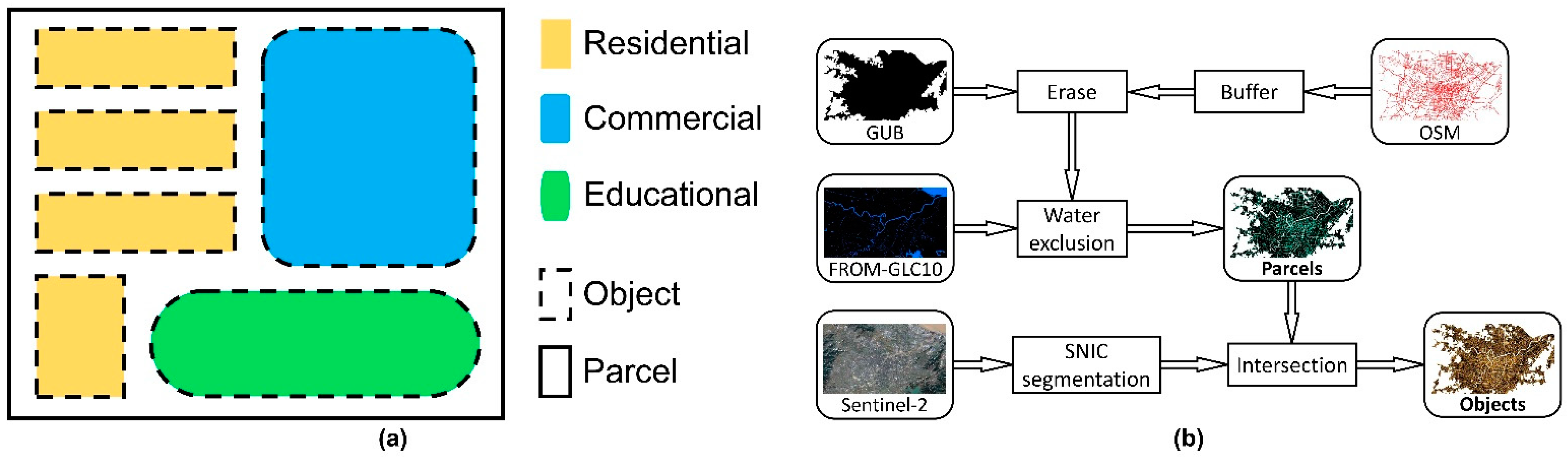
2.1. Basic Assumption: Each Parcel Is Composed of Objects

The starting point of our two-stage urban land use mapping framework lies in the spatial structure of mapping units, that is, each parcel consists of several objects, which have the same or different land use attributes. Since a pixel does not explicitly represent an entity characterizing the urban environment, we exclude the pixel-scale context in this study. A parcel is defined as a geographically meaningful region with relatively homogeneous socioeconomic functions and is usually delineated by the road network that surrounds [12,39,41]. An object is defined as a group of pixels with consistent visual cues, such as spectrum, texture, and shape [24,36]. Normally, a parcel has a larger area than an object does. Figure 1a displays a conceptional example of spatial interdependence between parcels and objects, in which a parcel contains multiple objects with different urban land uses including residential areas, commercial areas, and educational areas. In some cases, parcels may be used for a single land use type, for example, all buildings within a land parcel being for residential purpose. We interpret such kinds of parcels (i.e., one with objects in it all having the same function) as relatively pure land use.
Figure 1b shows a flowchart for the generation of the two kinds of mapping units (i.e., the basic spatial context for urban land use classification in this study). We leveraged multiple datasets from OSM road network, global urban boundaries (GUB) [62], and the 10 m global land cover product (FROM-GLC10) [63] for generating parcels while adopting a seed-based segmentation approach called the simple non-iterative clustering (SNIC) algorithm [64] for segmenting the 10 m Sentinel-2 imagery into homogeneous objects. See Supplementary Material Section S1 for more information on the generation of two types of mapping units.

2.2. Stage-1: Mapping at the Object Scale

Figure 2 presents a flowchart outlining the entire mapping scheme. According to the basic assumption in Section 2.1, we divided this framework into mapping essential urban land use categories at two stages: the object scale (EULUC-seg, stage 1) and the parcel scale (EULUC-parcel, stage 2). In stage 1, four main procedures were involved (Figure 2): extracting features from multi-source remotely sensed and social sensing data; collecting training and validation samples; automatic classification with ensemble learning; and mapping and accuracy assessment. We performed ensemble learning and statistical analysis in the Python 3 environment and used the ArcMap 10.3 software for spatial analysis and map production.

2.2.1. Feature Extraction

The inclusive features can be divided into two categories: remote sensing based and social sensing based. For remote sensing images, the average value, the sum value, and the standard deviation of each band are the most commonly used features. Additionally, texture features that describe the degree of tonal variations across pixels of an image or the level of landscape heterogeneity of an area [65] is another widely adopted item of information in land use classification [15,20,22,66,67]. Among the numerous texture calculation approaches in the literature, the gray level co-occurrence matrix (GLCM) method proposed by Haralick et al. [68] is a reliable method that computes the texture of an image by counting the occurrences of combinations of specific values between neighborhood pixels [69]. Following the GLCM method, we calculated six texture metrics of variance, correlation, contrast, dissimilarity, entropy, and angular second moment in this study. Details about the metric calculation and descriptions are provided in Table S1.
As for social sensing data, feature extraction is determined by the structure and characteristics of data. For example, the point of interest (POI) data are a set of points recording multiple spatial and attribute information of geographical entities, such as addresses, names, coordinates, and land use types. In this case, features of POI data are usually calculated based on the number and proportion of each POI type within the mapping unit.
Table S2 summarizes all object-based features used in the stage 1 mapping of EULUC-seg. In total, 76 features derived from multi-source remotely sensed and social sensing data sources were included in this study.

2.2.2. Sample Collection

We adopted the two-level classification system proposed in our previous study for mapping urban land use, which comprises five major (Level I) categories (residential, commercial, industrial, transportation, and public) and twelve minor (Level II) categories (residential, village, business, commercial, industrial, transportation, administrative, educational, medical, sport and cultural, park and greenspace, and undeveloped) (Table 1). This classification system originated from the EULUC scheme proposed by Gong et al. [41] and was later modified by Tu et al. [23] considering the characteristics of the study area. Detailed descriptions for each category of the two-level EULUC classification system are provided in Table S3. Based on the defined classification system, we identified 485 samples of the ground truth through visual interpretation and field investigation (Table 1). Practically, we first randomly selected objects within the study area and interpreted them based on multiple online sources such as Google Earth (https://www.google.com/earth/, accessed on 20 August 2021) and Baidu Street View Maps (https://map.baidu.com/, accessed on 20 August 2021). Second, we conducted an on-site field survey back in October 2019 and confirmed that more than 99% of the investigated samples were correct [23]. For subsequent analysis, the collected samples were randomly split into two datasets, that is, 70% for training (340) and 30% for validation (145). The training data were used for ensemble learning through multi-layer stacking, 5-fold cross-validation, and parameter tuning (see Section 2.2.3). The optimal model retrieved from ensemble learning was then applied to the validation samples for an accuracy assessment (see Section 2.2.4).

2.2.3. Ensemble Learning

As shown in Figure 2, we leveraged the multi-layer stacking model in ensemble learning. Each stack layer (L) is composed of several individual base models (“Base Learner” (BL)) and a “Meta Learner” (ML). Iteratively, each base model in BLn is trained individually with the output of MLn−1 in the previous stack layer, and MLn is trained by stacking the learning results from BLn and original input features. The revisit of the original data enables high-layer stackers to achieve more robust and accurate performance during the training process.
Apart from multi-layer stacking, here we adopted a bagging approach called k-fold cross-validation for reducing variance in predicting results and mitigating over-fitting issues in ensemble learning. Practically, for any base model in BLn, we randomly partitioned the input dataset into k subsamples with equal size (stratified based on labels). Among the k subsamples, one single subsample was reserved as the validation set for model testing, and the remaining k−1 subsamples were used for model training. This cross-validation process would be repeated k times, in which each k subsample was used only once for the validation. The averaged k results were then computed as the final output.
We employed the AutoGluon package introduced by Erickson et al. [70] to realize automatic ensemble learning. AutoGluon is an open-source Python library that automates the process of model selection, hyperparameter tuning, and model ensembling during machine learning [70]. Based on the given parameters, such as training time, bagging strategy, etc., AutoGluon will automatically achieve the best classification results by combining and stacking multi-model classifications. In this study, the parameter “num_bag_folds” was set to 5 for 5-fold cross-validation, “auto_stack” was set to True for automatic multi-layer stacking, and “time_limit” was set to 3600 for a maximum learning time of 3600 s in total. To achieve the most robust classification results, we used all the available base models provided by AutoGluon herein ensemble learning, which included Random Forest [71], Extremely Randomized Trees [72], Gradient Boosted Decision Trees (CatBoost) [73], Light Gradient Boosting Machine (LightGBM) [74], and Neural Networks [75]. For each base model, we tested its performance under 20 sets of parameter combinations and chose values with the highest overall accuracy as the optimal parameters. An introduction to each base model as well as its parameter settings is provided in Supplementary Material Section S2.

2.2.4. Accuracy Assessment and Mapping

Two evaluation schemes were included in the accuracy assessment. For the training process, the average overall accuracy [76] derived from the 5-fold cross-validation using ensemble learning was calculated for comparing the classification performance of different models. In this process, the model with the highest training accuracy was defined as the optimal model. For the validation process, the validation sample set (described in Section 2.2.2) was used to assess the performance of the optimal model independently. Specifically, we calculated the overall accuracy, Kappa coefficient, user accuracy, and producer accuracy based on the confusion matrix [77].
After that, we predicted the land use categories based on the derived features (Section 2.2.1) and the optimal training model (Section 2.2.3), and finally generated the stage-1 mapping results of EULUC-seg.

2.3. Stage-2: Mapping at the Parcel Scale

Since each parcel consisted of several objects, we could further identify the land use attributes (dominant category, degree of mix, etc.) of parcels according to objects within them, which had been classified in the previous stage of EULUC-seg. Specifically, for stage 2 mapping of EULUC-parcel, we defined and calculated three indices, i.e., dominant category (DC), dominant rate (DR), and complexity index (CI), based on the spatial relationship between land parcels and objects. We assigned DC as the final map of EULUC-parcel. We used DR and CI to measure the land use mix of parcels.
Let Pi represent the area proportion of the i-th land use category to the entire parcel and n the total number of land use categories of a parcel. Three indices of DC, DR, and CI can be calculated as:
DC = argmax   i P i ,
DR = P D C ,
CI = i = 1 n P i ln ( P i ) / ln ( n ) ,
DC is determined as the land use category with the largest area proportion within each parcel. DR refers to the area proportion of DC in the entire parcel. The larger the DR, the purer the parcel (1 indicates single land use). CI is essentially an entropy-based index that characterizes the evenness of land use classes and has been widely adopted in measuring land use mix [50,60,78,79,80]. It ranges from 0 to 1 with a higher CI value indicating a more mixed parcel and vice versa. CI equals 0 when there is only one land use within the parcel and reaches 1 when all the land use classes are evenly distributed. In this study, we mainly focused on the calculation and analysis of land use mix for the Level I category.

2.4. Quantifying Influencing Factors of Land Use Mix

With an understanding of the current status of land use mix, our next goal was to explore the underlying factors behind the spatial heterogeneity of land use mix, which can provide guidance and insight for urban planning and neighborhood design. After a comprehensive review of the existing literature [51,57,61,81], we selected 19 variables from four aspects of geography, socioeconomy, accessibility, and landscape as the potential influencing factors of urban land use mix (Table 2). The variables, calculated at the parcel scale, were based on attributes of the landscape itself (e.g., parcel size), in addition to other multi-source geospatial data (e.g., using digital elevation model (DEM) data to obtain elevations). Taking the Level I category as an experiment, we further uncovered the driving forces of land use mix by performing principal components analysis (PCA) and multiple linear regression with CI as the dependent variable. A detailed description of how we processed and calculated the raw data to derive these variables as well as quantified their associations with land use mix was provided in the Supplementary Material Section S3.

3. Experimental Tests and Results

3.1. Study Area and Data
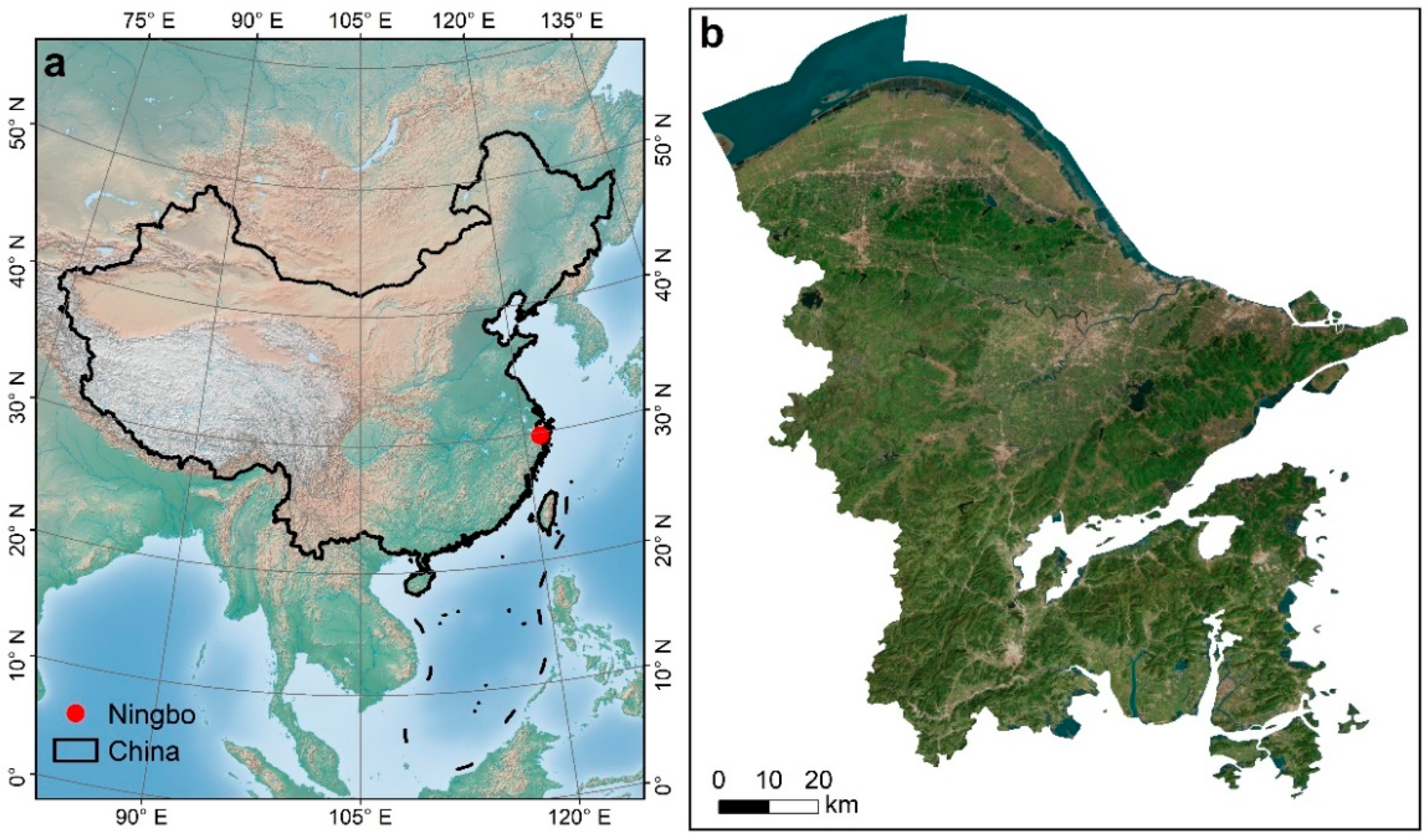
3.1.1. Study Area

Ningbo is a sub-provincial city located in the northeastern Zhejiang province, China (between 28°51′–30°33′N and 120°55′–122°16′E, Figure 3). It faces the East China Sea and Zhoushan Archipelago to the east, Hangzhou Bay to the north, and Shanghai—the largest and most prosperous metropolis in China—across the sea [82]. Topographically, the city is high in the southwest and low in the northeast with an average elevation of 4 m [83]. The total land area of Ningbo is 9816.23 km2, of which plain accounts for 40.3%, hill accounts for 25.2%, and mountain accounts for 24.9% [84].
Benefiting from the country’s “Reform and Opening-Up” policy, Ningbo is among the first batch of Chinese coastal cities that opened to the outside world back in the 1980s. It has, therefore, been experiencing dramatic socioeconomic development, rapid urban expansion, and substantial population growth in the past four decades. Statistically, Ningbo’s gross domestic product (GDP) has increased from USD 0.37 billion in 1979 to USD 191.68 billion in 2020. It now possesses a registered population of 6.03 million with an urbanization rate of 72.9% [85]. As an important economic, industrial, and trading center in East China, the city has a diversified land use pattern [23,84,86], making it a representative region for case studies.

3.1.2. Data

As listed in Table 3, we included an expansive set of remotely sensed and social sensing data layers for mapping urban land use categories, including Sentinel-1 Synthetic Aperture Radar (SAR) imagery, Sentinel-2 multispectral imagery, Luojia-1 NTL imagery, WorldPop population dataset, and Baidu POI data. All these datasets were collected during the year 2018 for temporal consistency. Details for the preparation and processing of each category of the used datasets are provided in the Supplementary Material Section S4. Figure S2 displays and compares six layers of the datasets used in the city center of Ningbo, in which a significant difference is observed in spectral reflectance, spatial resolution, and data structure. Compared with Sentinel-1 and Sentinel-2 (Figure S2a–c), Luojia-1 and WorldPop reveal fewer spatial details due to the relatively low spatial resolution (Figure S2d,e). As the only vector dataset used, the distribution of POI data shows a certain heterogeneity across space (Figure S2f). Following Section 2.2.1, we further extracted an expansive set of spectrum, texture, and additional features based on these datasets for object-based urban land use classification (i.e., stage 1 mapping). Figure S3 provides an example of the five typical object-based features derived.

3.2. Results

3.2.1. Accuracy Assessment

Table 4 and Table 5 compare the classification accuracy of different models of EULUC-seg for the two-level categories. At the object scale, Ensemble models achieved the best performance for both the Level I category (training accuracy: 86.47%) and the Level II category (training accuracy: 77.94%), followed by Neural Networks, LightGBM, CatBoost, Extremely Randomized Trees, and Random Forest models with slightly lower accuracy. This indicated that the multi-layer stacking strategy did help improve model performance in land use classification. Another finding was that Ensemble and Neural Networks models required more training time than other models. Given the relatively superior performance of Ensemble models, we chose them as the optimal models for subsequent analysis.
We further evaluated the classification performance of optimal models for each land use category in EULUC-seg, using the validation sample set in Section 2.2.2. An overall accuracy of 85.52% and a kappa coefficient of 0.79 were obtained for the five Level I categories (Table S5). Residential land had the highest user accuracy of 97.73%, while transportation land had the lowest user accuracy of 71.43%. In terms of producer accuracy, the classification performance of all Level I categories was rather satisfying (>85%). As for the Level II category, the overall accuracy and the kappa coefficient were 77.93% and 0.75, respectively (Table S6). Out of the twelve Level II categories, residential, village, and greenspace could be well classified, with both user accuracy and producer accuracy higher than 80%. In contrast, public land uses such as educational, medical, and sport and cultural lands yielded less plausible classification performance. As shown in the confusion matrix in Table S6, such kinds of land use categories, which aim at public management and service, can be easily confused with residential and business lands. Moreover, it was discovered that commercial lands had a relatively low user accuracy (41.67%), while industrial lands had a relatively low producer accuracy (60.00%).

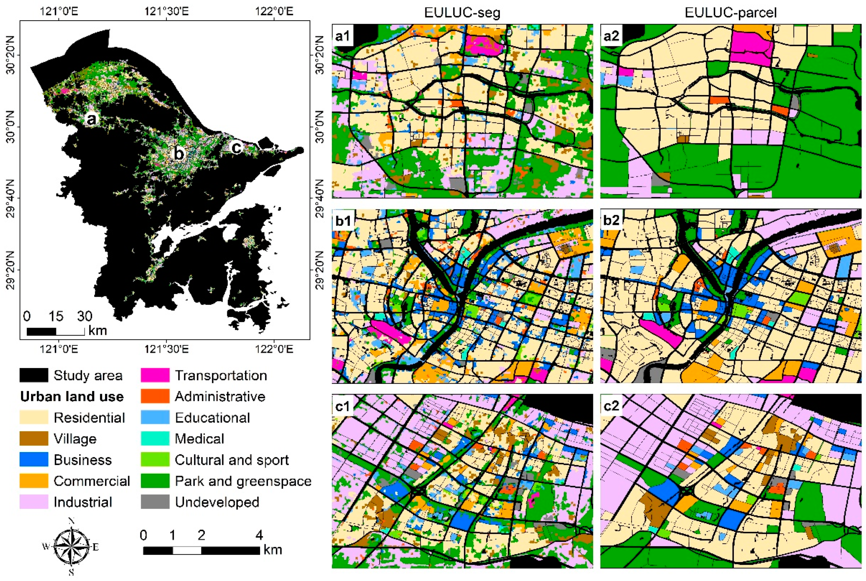
3.2.2. Mapping of Essential Urban Land Use Categories

Figure 4 shows the two-stage urban land use mapping results for Level II categories in Ningbo. Compared with EULUC-parcel, EULUC-seg was more fragmented with smaller mapping units. Owing to the proposed bottom-up mapping scheme, urban land use distributions showed good spatial consistency between the object scale and the parcel scale. The core urban area was dominated by residential, business, and commercial lands (Figure 4b1,b2), whereas the suburban area was mainly distributed with residential, village, industrial, and greenspace lands (Figure 4a1,a2,c1,c2). Table S7 summarizes the statistics of urban land use composition at the object scale. Statistically, within the 1441.27 km2 urban area of Ningbo, residual lands accounted for 30.17% (434.83 km2), commercial lands accounted for 2.68% (38.61 km2), industrial lands accounted for 20.03% (288.71 km2), transportation lands accounted for 0.99% (14.22 km2), and public lands accounted for 46.13% (664.90 km2). Overall, these results were essentially in accordance with our previous research [23].
Figure 5 distributes land use mix in Ningbo as well as its relationship with parcel size. In terms of spatial distribution, land use was heterogeneously mixed in the city center, with larger parcels generally having higher CI values (Figure 5a) and lower DR values (Figure 5b). This was confirmed in the linear regression results, where a significantly positive relationship (r = 0.57, p < 0.01) was observed between CI and parcel area (Figure 5c), while a significantly negative relationship (r = −0.60, p < 0.01) was observed between DR and parcel area (Figure 5d). Moreover, it was discovered that land use was relatively mixed in peri-urban areas, with CI values generally higher than 0.6 (Figure 5a).
Table 6 compares the degree of mix between different land use categories. Land uses for industrial and transportation purposes were the most complicated, with an average CI value of 0.56 ± 0.29 and 0.49 ± 0.35 and an average DR value of 0.76 ± 0.17 and 0.73 ± 0.23, respectively. In contrast, public lands had the simplest use among all categories, with a minimum CI value of 0.31 ± 0.37 and the maximum DR value of 0.87 ± 0.18. Moreover, residential and commercial lands were relatively simple, with half of them having a DR value higher than 0.86. In general, among the 5562 parcels investigated, most of them were dominated by one land use category only (average DR value: 0.84 ± 0.18) and about a quarter of them had a CI value greater than 0.71.

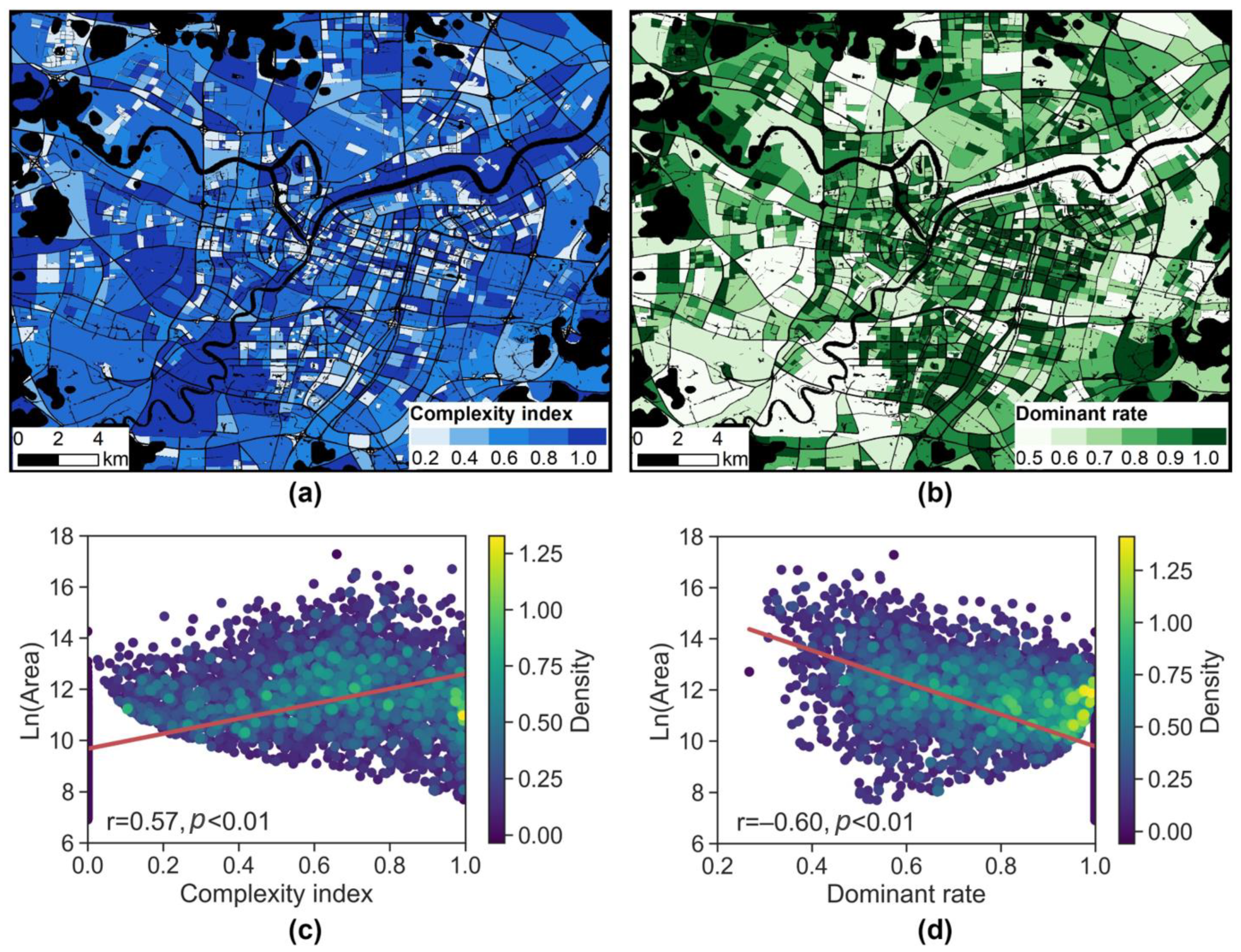
3.2.3. Influencing Factors of Land Use Mix

Table 7 summarizes the extracted ten components from PCA, which totally explain 93.68% of the variables listed in Table 2. According to the calculated variable weights of different PCs (Table S8), we defined variables with loading factors greater than 0.5 as important variables and assigned physical meaning to each PC. For example, PC1 and PC2, which accounted for 39.17% and 16.59% of the overall variance in the original data, respectively, were both mainly explained by the variable of distance to subway station (dis_subway). Therefore, these two components could be generally grouped as accessibility.
Table 8 reports the results of the multiple linear regression model with complexity index CI as the dependent variable. Both PC1 and PC2, which represented the accessibility aspect, were significantly associated with the complexity index in a positive manner, indicating that the longer the distance to the subway station, the larger the land use mix will be. Contrary to the subway, regression results of PC3 showed that the complexity of parcels would increase when their distances to the track road or the railway decreased (p < 0.05), a negative relationship. These results of PC1–3 indicated that accessibility had a double-edged impact on land use. PC8 was negatively associated with the complexity index at the p < 0.001 level, implying parcels with higher house prices and more irregular shapes would have less mixed land use. Moreover, regression results of PC4 and PC6 both reflected that a friendlier natural environment (such as higher green cover rates) could lead to an increase in land use mix.

4. Discussion

4.1. Advantages of the Proposed Framework

Different from previous studies that only focused on a single mapping scale, in this research, we identified land use attributes at both parcel and object scales using a bottom-up mapping strategy, with the aid of multi-source geospatial big data and ensemble learning approaches. The developed mapping scheme has some noticeable advantages. First, it significantly improves classification accuracy at the object scale. Machine learning has been widely accepted as a fundamental tool for land use and land cover classification. In this study, leveraging the automatic ensemble learning strategy, we tested a group of machine learning algorithms and compared multi-model performance in urban land use classification, using the same training and validation samples. Our results showed that Ensemble models achieved more robust and better performance in terms of classification accuracy. Compared with other models, the utilization of Ensemble models could yield a net increase in the training accuracy of 2.65–6.18% for the Level I category and 2.65%–8.53% for the Level II category (Table 4 and Table 5). Since the protocol of ensemble learning is to incorporate results of various models through multi-layer stacking and bagging, this method is especially suitable for dealing with extensive data with high dimensions. The efficiency and robustness of machine learning have also been observed and discussed in our previous experiments for land use and land cover mapping [12,23,44,87,88,89].
Second, the proposed scheme has, in the meantime, achieved robust classification results at the parcel scale. Mixed land use has been a major challenge in parcel-based land use mapping. In the nationwide study of EULUC-China, for instance, Gong et al. [41] discovered that overall accuracy decreases rapidly with the increase in the land use mix of parcels. Figure S4 also provides a comparison between the two-stage mapping results of this study with the EULUC-China maps [41]. Since Gong et al. [41] directly performed classification at the parcel scale, parcels with mixed land use, especially large ones, were easily misclassified (Figure S4j–l). By addressing this shortcoming, our mapping results will be more accurate in revealing land use patterns and keep solid spatial consistency between objects (Figure S4d–f) and parcels (Figure S4g–i).
Third, the proposed mapping framework has offered an alternative to measuring land use mix. At the parcel scale, we delineated the degree of land use mix (CI) and the rate of dominant land use (DR) through spatial aggregation and indices calculation, using the classification results at the object scale. We found that larger parcels had more mixed land use, of which many were distributed in the peri-urban area (Figure 5). We also found that industrial land uses were the most complicated, while residential and public lands were the simplest land uses (Table 6). These findings were generally in line with previous research [51,80]. Theoretically, the proposed scheme is very flexible and can be extended to any other region in the future. Based on the generated land use maps, urban planners, decision-makers, and stakeholders may use them as a benchmark to understand the current distribution, rationality, and mixture of land use or to examine the implementation effects of land adjustment and planning policy. Moreover, the produced maps can be correlated with factors such as urban livability or environmental quality to explore the potential influencing factors of mixed land use, which in turn guide future urban planning.

4.2. Limitations and Future Work

A few remaining caveats caused by data limitations need to be acknowledged. On the one hand, the size of mapping units largely depends on the data quality and parameter settings. For instance, parcels in this study are generated based on buffered roads of OSM data (Figure 1b). For areas where OSM roads are sparse or even absent, the generated parcels can be too large and are not suitable for urban studies. On the other hand, this study focuses on the spatial complexity of different land use categories but neglects other kinds of mixes (such as horizontal mix or inner mix). In reality, it is common in urban planning that a building provides both commercial and residential functions. To deeper uncover the nature of urban land use composition, higher-quality emerging data (such as street view maps) and more refined models (such as the 3D model) are urgently needed in future work. Lastly, our experiments and analysis focus on one Chinese city of Ningbo given the cost of sample collections and data availability, and the results and conclusions may not be applicable to other cities. Nonetheless, the main purpose of this research is to develop a prototype that comprehensively examines the distribution, mixture, and factors of urban land use. Potentially through crowdsourcing and cross-cooperation, our next goal is to de-composite land use patterns across cities with different socioeconomic development and historical-cultural backgrounds, which provides new insights into urban planning and management at a broader scale.

5. Conclusions

Leveraging multi-source open big data and machine learning algorithms, this research developed a flexible and cost-effective framework for multi-scale urban land use category mapping. Following this framework, we first performed object-based land use classification using an expansive set of remote sensing and social sensing data layers including OSM, Sentinel-1, Sentinel-2, Luojia-1, WorldPop, and Baidu POI data. Secondly, by spatially joining the classification results from the object scale, we calculated three land use attributes including dominant category, dominant rate, and complexity index at the parcel scale. Our results indicated that Ensemble models achieved better results than the other base models, with a training accuracy of 86% for the Level I category and 78% for the Level II category, respectively. In addition, the two-stage mapping results showed strong consistency in spatial patterns. These findings elucidated the role of multi-layer stacking and bagging in urban land use classifications.
Land use mix, as a ubiquitous characteristic of cities, has become a key concern in recent urban planning. Here, we proposed an efficient approach to measuring the degree of land use mix and its underlying driving forces. With this detailed information, planners, stakeholders, and city officials can quickly understand current land use compositions as well as decide when and where adjustments should be made. The new framework is expected to be widely utilized in various applications and implications across regions and countries.

Supplementary Materials

The following are available online at https://www.mdpi.com/article/10.3390/rs13214241/s1, Section S1: Mapping units generation, Section S2: Base models and parameter tuning in ensemble learning, Section S3: Quantifying influencing factors of land use mix, Section S4: Data preparation and processing, Table S1: Texture metrics used in this study, Table S2: Summary of features used in the stage-1 mapping of EULUC-seg, Table S3: The two-level essential urban land use categories (EULUC) classification system, Table S4: Tuned optimal parameters for each base model in ensemble learning, Table S5: Confusion matrix for the Level I category of EULUC-seg, Table S6: Confusion matrix for the Level II category of EULUC-seg, Table S7: Urban land use composition in Ningbo, 2018, Table S8: Extracted ten components from PCA and their variable weights, Figure S1: The architecture of Neural Networks in ensemble learning, Figure S2: Comparison of multi-source data with different spatial resolutions used for urban land use classification in this study, Figure S3: Comparison of object-based features derived from multi-source data in the city center of Ningbo, Figure S4: Comparison of remotely sensed images and urban land use mapping results.

Author Contributions

Conceptualization, Y.T. and B.C.; methodology, Y.T.; software, Y.T.; validation, Y.T.; formal analysis, Y.T.; investigation, Y.T. and T.Z.; resources, Y.T.; data curation, Y.T.; writing—original draft preparation, Y.T.; writing—review and editing, B.C., W.L., T.C., M.L. and B.X.; visualization, Y.T.; supervision, B.X.; project administration, B.X.; funding acquisition, B.C. and B.X. All authors have read and agreed to the published version of the manuscript.

Funding

This study was supported by the Major Program of the National Natural Science Foundation of China (20201321441), The University of Hong Kong HKU-100 Scholars Fund, and the National Natural Science Foundation of China (41801161, 41801163).

Data Availability Statement

Interactive map for the Level I categories of essential urban land use in Ningbo is available at https://thutyecology.users.earthengine.app/view/euluc-ningbo-viewer (accessed on 20 August 2021).

Conflicts of Interest

The authors declare no conflict of interest.

References

  1. Gong, P.; Li, X.; Wang, J.; Bai, Y.; Chen, B.; Hu, T.; Liu, X.; Xu, B.; Yang, J.; Zhang, W.; et al. Annual Maps of Global Artificial Impervious Area (GAIA) between 1985 and 2018. Remote Sens. Environ. 2020, 236, 111510. [Google Scholar] [CrossRef]
  2. United Nations, Department of Economic and Social Affairs, Population Division. World Population Prospects 2019: Highlights; United Nations: New York, NY, USA, 2019; p. 40. [Google Scholar]
  3. United Nations. World Urbanization Prospects 2018: Highlights. 2018. Available online: https://population.un.org/wup/Publications/Files/WUP2018-Highlights.pdf (accessed on 20 August 2021).
  4. Grimm, N.B.; Faeth, S.H.; Golubiewski, N.E.; Redman, C.L.; Wu, J.; Bai, X.; Briggs, J.M. Global Change and the Ecology of Cities. Science 2008, 319, 756–760. [Google Scholar] [CrossRef] [PubMed] [Green Version]
  5. He, C.Y.; Gao, B.; Huang, Q.X.; Ma, Q.; Dou, Y.Y. Environmental degradation in the urban areas of China: Evidence from multi-source remote sensing data. Remote Sens. Environ. 2017, 193, 65–75. [Google Scholar] [CrossRef]
  6. Chen, B.; Nie, Z.; Chen, Z.; Xu, B. Quantitative estimation of 21st-century urban greenspace changes in Chinese populous cities. Sci. Total Environ. 2017, 609, 956–965. [Google Scholar] [CrossRef]
  7. Song, Y.; Chen, B.; Kwan, M.-P. How does urban expansion impact people’s exposure to green environments? A comparative study of 290 Chinese cities. J. Clean. Prod. 2020, 246, 119018. [Google Scholar] [CrossRef]
  8. Tu, Y.; Chen, B.; Yu, L.; Xin, Q.; Gong, P.; Xu, B. How does urban expansion interact with cropland loss? A comparison of 14 Chinese cities from 1980 to 2015. Landsc. Ecol. 2021, 36, 243–263. [Google Scholar] [CrossRef]
  9. Van Vliet, J. Direct and Indirect Loss of Natural Area from Urban Expansion. Nat. Sustain. 2019, 2, 755–763. [Google Scholar] [CrossRef]
  10. McDonald, R.I.; Kareivab, P.; Forman, R.T. The Implications of Current and Future Urbanization for Global Protected Areas and Biodiversity Conservation. Biol. Conserv. 2008, 141, 1695–1703. [Google Scholar] [CrossRef]
  11. McKinney, M.L. Urbanization, Biodiversity, and ConservationThe Impacts of Urbanization on Native Species are Poorly Studied, but Educating a Highly Urbanized Human Population about These Impacts can Greatly Improve Species Conservation in all Ecosystems. Bioscience 2002, 52, 883–890. [Google Scholar] [CrossRef]
  12. Chen, B.; Tu, Y.; Song, Y.; Theobald, D.M.; Zhang, T.; Ren, Z.; Li, X.; Yang, J.; Wang, J.; Wang, X.; et al. Mapping Essential Urban Land use Categories with Open Big Data: Results for Five Metropolitan Areas in the United States of America. ISPRS J. Photogramm. Remote Sens. 2021, 178, 203–218. [Google Scholar] [CrossRef]
  13. Chen, B.; Xu, B.; Gong, P. Mapping Essential Urban Land Use Categories (Euluc) Using Geospatial Big Data: Progress, Challenges, and Opportunities. Big Earth Data 2021, 5, 410–441. [Google Scholar] [CrossRef]
  14. Gong, P.; Howarth, P.J. Land-Use Classification of SPOT HRV Data Using a Cover-Frequency Method. Int. J. Remote Sens. 1992, 13, 1459–1471. [Google Scholar] [CrossRef]
  15. Gong, P.; Marceau, D.J.; Howarth, P.J. A Comparison of Spatial Feature Extraction Algorithms for Land-Use Classification with SPOT HRV Data. Remote Sens. Environ. 1992, 40, 137–151. [Google Scholar] [CrossRef]
  16. Lu, D.; Weng, Q. Use of Impervious Surface in Urban Land-Use Classification. Remote Sens. Environ. 2006, 102, 146–160. [Google Scholar] [CrossRef]
  17. Myint, S.W.; Wentz, E.A.; Purkis, S.J. Employing Spatial Metrics in Urban Land-Use/Land-Cover Mapping. Photogramm. Eng. Remote Sens. 2007, 73, 1403–1415. [Google Scholar] [CrossRef]
  18. Pacifici, F.; Chini, M.; Emery, W. A Neural Network Approach Using Multi-Scale Textural Metrics from Very High-Resolution Panchromatic Imagery for Urban land-Use Classification. Remote Sens. Environ. 2009, 113, 1276–1292. [Google Scholar] [CrossRef]
  19. Theobald, D.M. Development and Applications of a Comprehensive Land Use Classification and Map for the US. PLoS ONE 2014, 9, e94628. [Google Scholar] [CrossRef] [PubMed] [Green Version]
  20. Herold, M.; Liu, X.; Clarke, K. Spatial Metrics and Image Texture for Mapping Urban Land Use. Photogramm. Eng. Remote Sens. 2003, 69, 991–1001. [Google Scholar] [CrossRef] [Green Version]
  21. Petropoulos, G.P.; Kalaitzidis, C.; Vadrevu, K. Support Vector Machines and Object-Based Classification for Obtaining Land-Use/Cover Cartography from Hyperion Hyperspectral Imagery. Comput. Geosci. 2012, 41, 99–107. [Google Scholar] [CrossRef]
  22. Hernandez, I.E.R.; Shi, W. A Random Forests Classification Method for Urban Land-Use Mapping Integrating Spatial Metrics and Texture Analysis. Int. J. Remote Sens. 2017, 39, 1175–1198. [Google Scholar] [CrossRef]
  23. Tu, Y.; Chen, B.; Zhang, T.; Xu, B. Regional Mapping of Essential Urban Land Use Categories in China: A Segmentation-Based Approach. Remote Sens. 2020, 12, 1058. [Google Scholar] [CrossRef] [Green Version]
  24. Blaschke, T. Object Based Image Analysis for Remote Sensing. ISPRS J. Photogramm. Remote Sens. 2010, 65, 2–16. [Google Scholar] [CrossRef] [Green Version]
  25. Liu, D.; Xia, F. Assessing Object-Based Classification: Advantages and Limitations. Remote Sens. Lett. 2010, 1, 187–194. [Google Scholar] [CrossRef]
  26. LeCun, Y.; Bengio, Y.; Hinton, G. Deep Learning. Nature 2015, 521, 436–444. [Google Scholar] [CrossRef] [PubMed]
  27. Schmidhuber, J. Deep Learning in Neural Networks: An Overview. Neural Netw. 2015, 61, 85–117. [Google Scholar] [CrossRef] [PubMed] [Green Version]
  28. Ma, L.; Liu, Y.; Zhang, X.; Ye, Y.; Yin, G.; Johnson, B.A. Deep Learning in Remote Sensing Applications: A Meta-Analysis and Review. ISPRS J. Photogramm. Remote Sens. 2019, 152, 166–177. [Google Scholar] [CrossRef]
  29. Huang, B.; Zhao, B.; Song, Y. Urban Land-Use Mapping Using a Deep Convolutional Neural Network with High Spatial Resolution Multispectral Remote Sensing Imagery. Remote Sens. Environ. 2018, 214, 73–86. [Google Scholar] [CrossRef]
  30. Zhang, C.; Sargent, I.; Pan, X.; Li, H.; Gardiner, A.; Hare, J.; Atkinson, P. An Object-Based Convolutional Neural Network (OCNN) for Urban Land Use Classification. Remote Sens. Environ. 2018, 216, 57–70. [Google Scholar] [CrossRef] [Green Version]
  31. Liu, S.; Qi, Z.; Li, X.; Yeh, A.G.-O. Integration of Convolutional Neural Networks and Object-Based Post-Classification Refinement for Land Use and Land Cover Mapping with Optical and SAR Data. Remote Sens. 2019, 11, 690. [Google Scholar] [CrossRef] [Green Version]
  32. Srivastava, S.; Vargas-Muñoz, J.E.; Tuia, D. Understanding Urban Landuse from the Above and Ground Perspectives: A Deep Learning, Multimodal Solution. Remote Sens. Environ. 2019, 228, 129–143. [Google Scholar] [CrossRef] [Green Version]
  33. Zhang, C.; Sargent, I.M.J.; Pan, X.; Li, H.; Gardiner, A.; Hare, J.; Atkinson, P.M. Joint Deep Learning for Land Cover and Land Use Classification. Remote Sens. Environ. 2019, 221, 173–187. [Google Scholar] [CrossRef] [Green Version]
  34. Bao, H.; Ming, D.; Guo, Y.; Zhang, K.; Zhou, K.; Du, S. DFCNN-Based Semantic Recognition of Urban Functional Zones by Integrating Remote Sensing Data and POI Data. Remote Sens. 2020, 12, 1088. [Google Scholar] [CrossRef] [Green Version]
  35. Atwell, W.; Rojdev, K.; Aghara, S.; Sriprisan, S. Mitigating the Effects of the Space Radiation Environment: A Novel Approach of Using Graded-Z Materials. In AIAA SPACE 2013 Conference & Exposition; American Institute of Aeronautics and Astronautics: Reston, VI, USA, 2013. [Google Scholar] [CrossRef]
  36. Myint, S.W.; Gober, P.; Brazel, A.; Grossman-Clarke, S.; Weng, Q. Per-Pixel Vs. Object-Based Classification of Urban Land Cover Extraction Using High Spatial Resolution Imagery. Remote Sens. Environ. 2011, 115, 1145–1161. [Google Scholar] [CrossRef]
  37. Zhong, Y.; Su, Y.; Wu, S.; Zheng, Z.; Zhao, J.; Ma, A.; Zhu, Q.; Ye, R.; Li, X.; Pellikka, P.; et al. Open-Source Data-Driven Urban Land-Use Mapping Integrating Point-Line-Polygon Semantic Objects: A Case Study of Chinese Cities. Remote Sens. Environ. 2020, 247, 111838. [Google Scholar] [CrossRef]
  38. Erol, H.; Akdeniz, F. A Per-Field Classification Method Based on Mixture Distribution Models and an Application to Landsat Thematic Mapper Data. Int. J. Remote Sens. 2005, 26, 1229–1244. [Google Scholar] [CrossRef]
  39. Liu, X.; Long, Y. Automated Identification and Characterization of Parcels with OpenStreetMap and Points of Interest. Environ. Plan. B Plan. Des. 2015, 43, 341–360. [Google Scholar] [CrossRef]
  40. Hu, T.; Yang, J.; Li, X.; Gong, P. Mapping Urban Land Use by Using Landsat Images and Open Social Data. Remote Sens. 2016, 8, 151. [Google Scholar] [CrossRef]
  41. Gong, P.; Chen, B.; Li, X.; Liu, H.; Wang, J.; Bai, Y.; Chen, J.; Chen, X.; Fang, L.; Feng, S.; et al. Mapping Essential Urban Land Use Categories in China (EULUC-China): Preliminary Results for 2018. Sci. Bull. 2020, 65, 182–187. [Google Scholar] [CrossRef] [Green Version]
  42. Polikar, R. Ensemble Learning. In Ensemble Machine Learning; Springer: Berlin/Heidelberg, Germany, 2012; pp. 1–34. [Google Scholar]
  43. Sagi, O.; Rokach, L. Ensemble Learning: A Survey. Wiley Interdiscip. Rev. Data Min. Knowl. Discov. 2018, 8, 1249. [Google Scholar] [CrossRef]
  44. Liu, H.; Gong, P.; Wang, J.; Wang, X.; Ning, G.; Xu, B. Production of Global Daily Seamless Data Cubes and Quantification of Global Land Cover Change from 1985 to 2020—Imap World 1.0. Remote Sens. Environ. 2021, 258, 112364. [Google Scholar] [CrossRef]
  45. Fan, R.; Feng, R.; Wang, L.; Yan, J.; Zhang, X. Semi-MCNN: A Semisupervised Multi-CNN Ensemble Learning Method for Urban Land Cover Classification Using Submeter HRRS Images. IEEE J. Sel. Top. Appl. Earth Obs. Remote Sens. 2020, 13, 4973–4987. [Google Scholar] [CrossRef]
  46. Cai, Y.; Li, X.; Zhang, M.; Lin, H. Mapping Wetland Using the Object-Based Stacked Generalization Method Based on Multi-temporal Optical and SAR Data. Int. J. Appl. Earth Obs. Geoinf. 2020, 92, 102164. [Google Scholar] [CrossRef]
  47. Wen, L.; Hughes, M. Coastal Wetland Mapping Using Ensemble Learning Algorithms: A Comparative Study of Bagging, Boosting and Stacking Techniques. Remote Sens. 2020, 12, 1683. [Google Scholar] [CrossRef]
  48. Wang, X.; Liu, S.; Du, P.; Liang, H.; Xia, J.; Li, Y. Object-Based Change Detection in Urban Areas from High Spatial Resolution Images Based on Multiple Features and Ensemble Learning. Remote Sens. 2018, 10, 276. [Google Scholar] [CrossRef] [Green Version]
  49. Cui, B.; Zhang, Y.; Yan, L.; Wei, J.; Wu, H. An Unsupervised SAR Change Detection Method Based on Stochastic Subspace Ensemble Learning. Remote Sens. 2019, 11, 1314. [Google Scholar] [CrossRef] [Green Version]
  50. Song, Y.; Merlin, L.; Rodriguez, D. Comparing Measures of Urban Land Use Mix. Comput. Environ. Urban Syst. 2013, 42, 1–13. [Google Scholar] [CrossRef]
  51. Tian, L.; Liang, Y.; Zhang, B. Measuring Residential and Industrial Land Use Mix in the Peri-Urban Areas of China. Land Use Policy 2017, 69, 427–438. [Google Scholar] [CrossRef]
  52. Abdullahi, S.; Pradhan, B.; Mansor, S.; Shariff, A.R.M. GIS-Based Modeling for the Spatial Measurement and Evaluation of Mixed Land Use Development for a Compact City. GIScience Remote Sens. 2015, 52, 18–39. [Google Scholar] [CrossRef]
  53. He, J.; Li, X.; Liu, P.; Wu, X.; Zhang, J.; Zhang, D.; Liu, X.; Yao, Y. Accurate Estimation of the Proportion of Mixed Land Use at the Street-Block Level by Integrating High Spatial Resolution Images and Geospatial Big Data. IEEE Trans. Geosci. Remote Sens. 2021, 59, 6357–6370. [Google Scholar] [CrossRef]
  54. Zhuo, Y.; Zheng, H.; Wu, C.; Xu, Z.; Li, G.; Yu, Z. Compatibility Mix Degree Index: A Novel Measure to Characterize Urban Land Use Mix Pattern. Comput. Environ. Urban Syst. 2019, 75, 49–60. [Google Scholar] [CrossRef]
  55. Jacobs, J. The Death and Life of Great American Cities; Vintage: New York, NY, USA, 2016. [Google Scholar]
  56. Kitamura, R.; Mokhtarian, P.L.; Daidet, L. A Micro-Analysis of Land Use and Travel in Five Neighborhoods in the San Francisco Bay Area. Transportation 1997, 24, 125–158. [Google Scholar] [CrossRef]
  57. Duncan, M.J.; Winkler, E.; Sugiyama, T.; Cerin, E.; Dutoit, L.; Leslie, E.; Owen, N. Relationships of Land Use Mix with Walking for Transport: Do Land Uses and Geographical Scale Matter? J. Hered. 2010, 87, 782–795. [Google Scholar] [CrossRef] [Green Version]
  58. Jia, P.; Pan, X.; Liu, F.; He, P.; Zhang, W.; Liu, L.; Zou, Y.; Chen, L. Land Use Mix in the Neighbourhood and Childhood Obesity. Obes. Rev. 2021, 22, 13098. [Google Scholar] [CrossRef]
  59. Frank, L.D.; Schmid, T.L.; Sallis, J.F.; Chapman, J.; Saelens, B.E. Linking Objectively Measured Physical Activity with Objectively Measured Urban form: Findings from SMARTRAQ. Am. J. Prev. Med. 2005, 28, 117–125. [Google Scholar] [CrossRef] [PubMed]
  60. Kong, H.; Sui, D.Z.; Tong, X.; Wang, X. Paths to Mixed-Use Development: A Case Study of Southern Changping in Beijing, China. Cities 2015, 44, 94–103. [Google Scholar] [CrossRef]
  61. Comer, D.; Greene, J.S. The Development and Application of a Land Use Diversity Index for Oklahoma City, OK. Appl. Geogr. 2015, 60, 46–57. [Google Scholar] [CrossRef]
  62. Li, X.; Gong, P.; Zhou, Y.; Wang, J.; Bai, Y.; Chen, B.; Hu, T.; Xiao, Y.; Xu, B.; Yang, J.; et al. Mapping Global Urban Boundaries from the Global Artificial Impervious Area (GAIA) Data. Environ. Res. Lett. 2020, 15, 094044. [Google Scholar] [CrossRef]
  63. Gong, P.; Liu, H.; Zhang, M.; Li, C.; Wang, J.; Huang, H.; Clinton, N.; Ji, L.; Li, W.; Bai, Y.; et al. Stable Classification with Limited Sample: Transferring a 30-m Resolution Sample Set Collected in 2015 to Mapping 10-m Resolution Global Land Cover in 2017. Sci. Bull. 2019, 64, 370–373. [Google Scholar] [CrossRef] [Green Version]
  64. Achanta, R.; Susstrunk, S. Superpixels and Polygons Using Simple Non-Iterative Clustering. In Proceedings of the 2017 IEEE Conference on Computer Vision and Pattern Recognition (CVPR), Honolulu, HI, USA, 21–26 July 2017; pp. 4895–4904, ISBN 1063-6919. [Google Scholar]
  65. Bhabatosh, C. Digital Image Processing and Analysis; PHI Learning Pvt. Ltd.: New Delhi, India, 1977. [Google Scholar]
  66. Xu, B.; Gong, P.; Seto, E.; Spear, R. Comparison of Gray-Level Reduction and Different Texture Spectrum Encoding Methods for Land-Use Classification Using a Panchromatic Ikonos Image. Photogramm. Eng. Remote Sens. 2003, 69, 529–536. [Google Scholar] [CrossRef]
  67. Wu, S.-S.; Qiu, X.; Usery, E.L.; Wang, L. Using Geometrical, Textural, and Contextual Information of Land Parcels for Classification of Detailed Urban Land Use. Ann. Assoc. Am. Geogr. 2009, 99, 76–98. [Google Scholar] [CrossRef]
  68. Haralick, R.M.; Shanmugam, K.; Dinstein, I. Textural Features for Image Classification. IEEE Trans. Syst. Man Cybern. 1973, SMC-3, 610–621. [Google Scholar] [CrossRef] [Green Version]
  69. Kupidura, P. The Comparison of Different Methods of Texture Analysis for Their Efficacy for Land Use Classification in Satellite Imagery. Remote Sens. 2019, 11, 1233. [Google Scholar] [CrossRef] [Green Version]
  70. Erickson, N.; Mueller, J.; Shirkov, A.; Zhang, H.; Larroy, P.; Li, M.; Smola, A. Autogluon-Tabular: Robust and Accurate Automl for Structured Data. arXiv 2020, arXiv:2003.06505. [Google Scholar]
  71. Breiman, L. Random Forests. Mach. Learn. 2001, 45, 5–32. [Google Scholar] [CrossRef] [Green Version]
  72. Geurts, P.; Ernst, D.; Wehenkel, L. Extremely Randomized Trees. Mach. Learn. 2006, 63, 3–42. [Google Scholar] [CrossRef] [Green Version]
  73. Dorogush, A.V.; Ershov, V.; Gulin, A. CatBoost: Gradient Boosting with Categorical Features Support. arXiv 2018, arXiv:1810.11363. [Google Scholar]
  74. Ke, G.; Meng, Q.; Finley, T.; Wang, T.; Chen, W.; Ma, W.; Ye, Q.; Liu, T.-Y. LightGBM: A Highly Efficient Gradient Boosting Decision Tree. 2017. Available online: https://proceedings.neurips.cc/paper/2017/file/6449f44a102fde848669bdd9eb6b76fa-Paper.pdf (accessed on 20 August 2021).
  75. Yegnanarayana, B. Artificial Neural Networks; PHI Learning Pvt. Ltd.: New Delhi, India, 2009. [Google Scholar]
  76. Congalton, R.G. A Review of Assessing the Accuracy of Classifications of Remotely Sensed Data. Remote Sens. Environ. 1991, 37, 35–46. [Google Scholar] [CrossRef]
  77. Congalton, R.G.; Green, K. Assessing the Accuracy of Remotely Sensed Data: Principles and Practices; CRC Press: Boca Raton, FL, USA, 2019. [Google Scholar]
  78. Jiao, J.; Rollo, J.; Fu, B. The Hidden Characteristics of Land-Use Mix Indices: An Overview and Validity Analysis Based on the Land Use in Melbourne, Australia. Sustainability 2021, 13, 1898. [Google Scholar] [CrossRef]
  79. Xing, H.; Meng, Y.; Shi, Y. A Dynamic Human Activity-Driven Model for Mixed Land Use Evaluation Using Social Media Data. Trans. GIS 2018, 22, 1130–1151. [Google Scholar] [CrossRef]
  80. Lang, W.; Long, Y.; Chen, T. Rediscovering Chinese Cities through the Lens of Land-Use Patterns. Land Use Policy 2018, 79, 362–374. [Google Scholar] [CrossRef]
  81. Yue, Y.; Zhuang, Y.; Yeh, A.G.-O.; Xie, J.-Y.; Ma, C.-L.; Li, Q.-Q. Measurements of POI-Based Mixed Use and Their Relationships with Neighbourhood Vibrancy. Int. J. Geogr. Inf. Sci. 2017, 31, 658–675. [Google Scholar] [CrossRef] [Green Version]
  82. Tang, Y.-T.; Chan, F.K.S.; Griffiths, J.A. City profile: Ningbo. Cities 2015, 42, 97–108. [Google Scholar] [CrossRef]
  83. Liang, H.; Guo, Z.; Wu, J.; Chen, Z. GDP Spatialization in Ningbo City based on NPP/VIIRS Night-Time Light and Auxiliary Data Using Random Forest Regression. Adv. Space Res. 2020, 65, 481–493. [Google Scholar] [CrossRef]
  84. Liu, Y.; Feng, Y.; Zhao, Z.; Zhang, Q.; Su, S. Socioeconomic Drivers of Forest Loss and Fragmentation: A Comparison between Different Land Use Planning Schemes and Policy Implications. Land Use Policy 2016, 54, 58–68. [Google Scholar] [CrossRef]
  85. Han, Y.; Yu, C.; Feng, Z.; Du, H.; Huang, C.; Wu, K. Construction and Optimization of Ecological Security Pattern Based on Spatial Syntax Classification—Taking Ningbo, China, as an Example. Land 2021, 10, 380. [Google Scholar] [CrossRef]
  86. Zhang, C.; Zhong, S.; Wang, X.; Shen, L.; Liu, L.; Liu, Y. Land Use Change in Coastal Cities during the Rapid Urbanization Period from 1990 to 2016: A Case Study in Ningbo City, China. Sustainability 2019, 11, 2122. [Google Scholar] [CrossRef] [Green Version]
  87. Chen, B.; Huang, B.; Xu, B. Multi-Source Remotely Sensed Data Fusion for Improving Land Cover Classification. ISPRS J. Photogramm. Remote Sens. 2017, 124, 27–39. [Google Scholar] [CrossRef]
  88. Chen, B.; Huang, B.; Xu, B. Fine Land Cover Classification Using Daily Synthetic Landsat-Like Images at 15-m Resolution. IEEE Geosci. Remote Sens. Lett. 2015, 12, 2359–2363. [Google Scholar] [CrossRef]
  89. Tu, Y.; Lang, W.; Yu, L.; Li, Y.; Jiang, J.; Qin, Y.; Wu, J.; Chen, T.; Xu, B. Improved Mapping Results of 10 m Resolution Land Cover Classification in Guangdong, China Using Multisource Remote Sensing Data With Google Earth Engine. IEEE J. Sel. Top. Appl. Earth Obs. Remote Sens. 2020, 13, 5384–5397. [Google Scholar] [CrossRef]
Figure 1. Relationship between parcels and objects. (a) An illustration of the spatial correlation between parcels and objects. A parcel can include several objects with different land uses, such as residential areas, commercial areas, and educational areas. (b) Processes for generating mapping units of parcels and objects. OSM: OpenStreetMap road network. GUB: global urban boundaries. FROM-GLC10: the 10 m global land cover product. SNIC: simple non-iterative clustering.
Remotesensing 13 04241 g001
Figure 2. Flowchart of the proposed two-stage urban land use mapping scheme.
Remotesensing 13 04241 g002
Figure 3. The study area of Ningbo. (a) Its geographical location in China. (b) High-resolution satellite image of Ningbo.
Remotesensing 13 04241 g003
Figure 4. The two-stage urban land use mapping results for Level II categories in Ningbo. (a1,a2) The Yuyao county located ~40 km west of the city center. (b1,b2) The central urban area of Ningbo where three main rivers (Fenghua river, Yong river, and Yao river) run through. (c1,c2) The Beilun district located ~30 km east of the city center.
Remotesensing 13 04241 g004
Figure 5. Land use mix of Level I categories in Ningbo. (a) Maps of complexity index in the city center. (b) Maps of dominant rate in the city center. (c) The relationship between complexity index and area of parcels. (d) The relationship between dominant rate and area of parcels. r in (c,d) represents the Pearson correlation coefficient.
Remotesensing 13 04241 g005
Table 1. Classification system and samples.
Level ILevel IINumber of Samples
01 Residential0101 Residential83
0102 Village50
02 Commercial0201 Business51
0202 Commercial33
03 Industrial0301 Industrial48
04 Transportation0401 Transportation20
05 Public0501 Administrative28
0502 Educational43
0503 Medical15
0504 Sport and cultural21
0505 Park and greenspace73
0506 Undeveloped20
Total 485
Table 2. Factors that influence land use mix. Noted all variables were calculated at the parcel scale.
AspectDescriptionVariableData SourceSpatial Resolution (m)
GeographyMean of elevationelevationSRTM DEM 230
Mean of NDVI 1ndviSentinel-210
Fraction of clayfra_claySoil texture data1000
Fraction of sandfra_sandSoil texture data1000
Fraction of siltfra_siltSoil texture data1000
SocioeconomyNumber of business pointsbusinessBaidu POI 3/
Number of commercial pointscommercialBaidu POI 3/
Mean of populationpopWorldPop100
Mean of nighttime lightntlLuojia-1130
Mean of house pricehouse_priceLianjia/
AccessibilityDistance to bus stationdis_busBaidu POI 3/
Distance to subway stationdis_subwayBaidu POI 3/
Distance to railwaydis_ railwayOSM 4±20
Distance to major roaddis_major_roadOSM 4±20
Distance to minor roaddis_minor_roadOSM 4±20
Distance to track roaddis_track_roadOSM 4±20
LandscapeArea of parcelarea//
Shape index of parcelshape//
Richness index of parcelrichness//
1 NDVI: normalized difference vegetation index. 2 SRTM DEM: shuttle radar topography mission digital elevation model. 3 POI: point of interest. 4 OSM: OpenStreetMap.
Table 3. An overview of datasets used for mapping urban land use.
CategoryData SourceResolution (m)Year
Synthetic Aperture RadarSentinel-1102018
MultispectralSentinel-210–602018
Nighttime lightLuojia-11302018
PopulationWorldPop1002018
Points of InterestBaidu POI/2018
Table 4. Level I accuracy comparison of different models of EULUC-seg in terms of training accuracy, training time, and stack level. Note the training accuracy is the average overall accuracy of the 5-fold cross-validation during training.
ModelTraining Accuracy (%)Training Time (s)Stack Level
Random Forest80.2985.571
Extremely Randomized Trees80.8868.461
CatBoost82.65232.771
LightGBM83.82168.001
Neural Networks86.474271.071
Ensemble86.474271.522
Table 5. Level II accuracy comparison of different models of EULUC-seg in terms of training accuracy, training time, and stack level. Note the training accuracy is the average overall accuracy of the 5-fold cross-validation during training.
ModelTraining Accuracy (%)Training Time (s)Stack Level
Random Forest69.4175.011
Extremely Randomized Trees72.3558.751
CatBoost72.06423.391
LightGBM74.41170.891
Neural Networks75.294356.121
Ensemble77.945279.672
Table 6. Statistics of complexity index and dominant rate for each Level I land use category. Definition for each land use category can be seen in Table 1.
Level IIndices
Complexity index
CountMeanSTD0%25%50%75%100%
0117670.370.360.000.000.330.701.00
025700.460.380.000.000.530.801.00
037220.560.290.000.400.610.761.00
041100.490.350.000.000.600.800.99
0524930.310.370.000.000.000.661.00
Total56620.380.370.000.000.360.711.00
Dominant rate
CountMeanSTD0%25%50%75%100%
0117670.850.170.320.720.931.001.00
025700.820.180.360.680.861.001.00
037220.760.170.270.630.790.901.00
041100.730.230.310.510.731.001.00
0524930.870.180.310.741.001.001.00
Total56620.840.180.270.700.921.001.00
Note. STD: standard deviation; x%: quantiles at the x% level.
Table 7. Summary of the extracted ten components from PCA. Important variables with a loading factor higher than 0.50 are listed.
ComponentPercentage of Explained Variances (%)Important VariablesPhysical Meanings
PC139.17dis_subwayaccessibility
PC216.59dis_subwayaccessibility
PC311.41dis_track_road, dis_railaccessibility
PC47.01ndvigeography
PC54.09richness, shapelandscape
PC63.99fra_siltgeography
PC73.74dis_major_roadaccessibility
PC83.37house_price, shapesocioeconomy and landscape
PC92.43dis_major_road, house_priceaccessibility and socioeconomy
PC101.89dis_railaccessibility
Total93.68
Table 8. Model report for the multiple linear regression analysis predicting Level I complexity index from the extracted ten components from PCA.
CoefficientSTDp ValueCI95
LLUL
Intercept41.40 ***0.550.00040.3342.48
PC15.17 ***1.430.0002.377.97
PC26.21 **2.190.0051.9110.52
PC3−6.51 *2.650.014−11.7−1.32
PC48.70 *3.380.0102.0715.34
PC5−7.234.420.102−15.881.43
PC610.80 *4.480.0162.0219.58
PC7−8.694.620.060−17.760.37
PC8−20.52 ***4.870.000−30.06−10.98
PC9−8.915.730.120−20.152.33
PC108.686.510.183−4.0921.45
Note. *** indicates p < 0.001, ** indicates p < 0.01, and * indicates p < 0.05. STD: standard deviation; CI95: 95% confidence interval; LL: lower limits of CI95; UL: upper limits of CI95.
Publisher’s Note: MDPI stays neutral with regard to jurisdictional claims in published maps and institutional affiliations.

