Recent Progress on Vegetation Remote Sensing Using Spaceborne GNSS-Reflectometry

Abstract

Vegetation is an important part of the terrestrial ecosystem and plays a vital role in the global carbon cycle. Traditional remote sensing methods have certain limitations in vegetation monitoring, and the development of GNSS-R (Global Navigation Satellite System-Reflectometry) technology provides a new and complimentary method. With the CYGNSS (Cyclone Global Navigation Satellite System) launch and the increased data acquisition, the use of spaceborne GNSS-R for vegetation monitoring has become a research hotspot. However, due to the complex characteristics of vegetation, its application in this field is still in the exploratory research stage. On the basis of reviewing the current research status, this paper points out the weak links of this technology in terms of polarization and observation geometry. Combined with the microwave vegetation scattering model, this paper analyzes the full polarization bistatic scattering characteristics of vegetation and points out the influence of vegetation parameters (density, water content, and vegetation diameters). The potential feasibility of polarization GNSS-R and future development trends of GNSS-R technology in quantitative retrieval (such as vegetation water content and biomass) are also discussed.

1. Introduction

The terrestrial ecosystem is the life support system that humans rely on for survival and development. Vegetation connects the atmosphere, water, and soil, and is an important part of the terrestrial ecosystem. It plays an indicator role in environmental changes and is an important component of the global carbon cycle. Therefore, it is urgent to carry out effective monitoring of key vegetation elements and related physical parameters and to explore its internal mechanism and existing laws in depth. However, the key vegetation parameters have strong temporal and spatial variation and non-uniformity. The traditional monitoring methods of base stations consume a lot of time and are costly. The development of satellite remote sensing technology provides new methods for monitoring.

Optical and thermal infrared remote sensing is limited by weather conditions and cannot work all day long. These limitations are overcome with microwave remote sensing. Due to its long wavelength, it has a certain degree of penetrability to rain clouds and can work under all-weather conditions. L-band satellites such as JERS-1 (Japanese Earth Resources Satellite-1), ALOS (Advanced Land Observing Satellite), and ALOS-2 can be used for vegetation monitoring, but the 6-week time resolution still limits their practical scientific applications.

GNSS (Global Navigation Satellite System) is a general term for various navigation satellite systems, including GPS (Global Positioning System) from the United States, GALILEO from Europe, GLONASS from Russia, and BDS (BeiDou Navigation Satellite System) from China. With the completion of the global network of China’s BDS in 2020, the number of existing navigation satellite signals in orbit will exceed more than 150. The traditional application of navigation satellites is to use their direct signals for positioning, navigation, and timing (PNT). However, since the direct signals are continuously reflected on the surface, they can be received by a special reflected signal receiver, forming a new remote sensing method: GNSS-R (GNSS-Reflectometry) remote sensing [1,2,3].

As for GNSS-R remote sensing, which employs the GNSS constellations as the transmitted signal source, this technique does not need dedicated transmitters. They only need the corresponding receivers to obtain the surface reflected signals. Therefore, the instruments of this kind of remote sensing technique have the salient features of being lightweight and requiring low power consumption. Because the GNSS constellation continuously emits direct signals, the spatiotemporal resolutions of this technique are much better than the traditional remote sensing techniques.

Compared with the complex medium on the land surface, the ocean surface is relatively uniform. The research of GNSS-R in the ocean field is earlier and more mature than in land surface. However, a data analysis using the UK-DMC (United Kingdom-Disaster Monitoring Constellation) satellite shows that the reflected signal from the land surface can be received [4]. Although the main scientific goal of CYGNSS (Cyclone Global Navigation Satellite System) launched by NASA in 2016 is to conduct sea surface hurricane research [5,6,7], its use for land surface parameter research has also become a hot topic in recent years [8,9,10]. On 5 July 2021, the Chinese meteorological satellite FY-3 E was successfully launched. There are eleven payloads on it, and one of them is the GNSS occultation and GNSS-R combined payload, whose potential scientific goal is for land surface remote sensing, and the corresponding research on land surface parameters (such as soil moisture and vegetation biomass) will be carried out in Henan Province simultaneously [11]. The Federated Satellite System mission (FSSCat) was the first Copernicus third-party mission based on CubeSats and it was launched in 2020. Flexible Microwave Payload-2 (FMPL-2) is its payload and it is a novel CubeSat based instrument combining an L1/E1 GNSS-R and an L-band Microwave Radiometer (MWR) using software-defined radio. Coarse Soil Moisture (SM) estimation is one of FSSCat’s objectives [12]. HydroGNSS is planned to be developed and launched before the end of 2024. This mission uses GNSS reflectometry to target four hydrological essential climate variables: soil moisture, wetland/inundation, freeze/thaw state, and above ground biomass [13].

Since GNSS-R is essentially a bistatic/multi-static radar operating in the L-band, and traditional microwave remote sensing has proven that this band is suitable for soil moisture observation [14,15], its current applications in land surface parameters are mostly concentrated on soil moisture [16,17,18,19,20,21]. Compared with traditional monostatic radar, the significant advantage of using this method to observe vegetation parameters is that the signal response to biomass will not be as easily saturated as in monostatic radar [22]. Therefore, the use of this remote sensing method to monitor vegetation parameters has advantages that traditional remote sensing methods cannot match. However, the changing observation geometry is one of the potential disadvantages of GNSS-R.

In this paper, we will summarize the current research status of GNSS-R vegetation remote sensing in Section 2. Meanwhile, the existing problems are discussed and analyzed in Section 3. Based on the microwave scattering characteristics, the future development trend is discussed in Section 4. Finally, we will give a conclusion in Section 5.

2. Research Status

Vegetation parameter monitoring and biomass inversion is a new research field of GNSS-R remote sensing technology. This section is going to give a comprehensive review of the development of the GNSS-R in vegetation study. Therefore, we have presented the development of GNSS-R on vegetation monitoring according to the platforms. Of course, at first, researchers indeed have presented works on the ground-based experiments, from which they have manifested that the vegetation parameters can be detected by the GNSS-R remote sensing technique (Section 2.1). Then, several works related to the airborne-GNSS-R vegetation campaigns have been carried out (Section 2.2). The scientific objectives of these works are related to the fact that the vegetation information can be obtained from airborne experiments. From the ground-based and airborne experiments, the researchers have proven the potentialities of this technique for vegetation study. Then, after the pioneer works have been done, the spaceborne missions have launched and a lot of space-borne data have become available to the scientific community and works related to vegetation study using spaceborne data have emerged (Section 2.3). At the same time, the development of mechanism models is an important research tool to promote the development of GNSS-R technology; therefore, we give a review of the research status of the GNSS-R vegetation model in detail (Section 2.4).

2.1. Ground-Based GNSS-R Vegetation Remote Sensing Research

The most representative research on vegetation parameters using a ground-based remote sensing platform is the GPS-SNR (Signal to Noise Ratio) method and IPT technique (Interference Pattern Technique). The former directly uses the multipath information received by the PBO (Plate Boundary Observatory) site to obtain SNR data, and extracts the effective reflectometer height, phase, and amplitude information, and then carries on the relevant vegetation inversion of water content and NMRI (Normalized Microwave Reflection Index) [23,24,25]. The latter employs an improved GPS receiver, that is, on the basis of the existing surveying and mapping receiver; however, they focus on improving the antenna polarization, and they have employed vertical polarization antenna to acquire the surface properties [26,27]. In order to improve the retrieval accuracy, they have also employed the horizontal polarization antenna for an analysis [28]. The receiver’s interference waveform is used to obtain vegetation height information by notch position and number information [26,27,28]. It should be noted that a GPS receiver intended to be used with the IPT technique obtains the constructive/destructive pattern of the combined reflected and direct signals.

2.2. Airborne GNSS-R Vegetation Remote Sensing Experiments

Two airborne experiments carried out by Egido et al. proved that when the biomass is as high as 300 ton/ha, there is still a correlation between the bistatic reflectivity and the biomass [29].

Under the funding of the SNSB (Swedish National Space Board) and ESA, researchers carried out the BEXUS 17 (Balloon Experiments for University Students) 25 Km stratospheric balloon experiment in the northern forests of Sweden on 10 October 2013 [30]. The experiments showed that the energy of the received reflected signal is basically independent of the height of the platform for a high coherent integration time (20 ms). The article [30] also suggested that the received coherent power comes from different forest elements (canopy, soil, etc).

The LEiMON (Land Monitoring with Navigation Signals) experiment was a 6-month GNSS-R experiment on ground-based crops conducted in the Florence agricultural area, Italy, from March to September 2009 [31]. The experiment used the SAM receiver developed by Barcelona Starlab Company, which was installed on a 25 m high hydraulic boom. This experiment compared and analyzed the relationship between surface roughness, soil moisture content, vegetation moisture content, and GNSS-R signal. The research shows that the correlation between reflected signals (both LR polarization and RR polarization) and vegetation moisture content is good (correlation coefficient is 0.8). It should be noted that here LR refers to the transmitted signal as right hand circular polarization (RHCP) and the received signal is left hand circular polarization (LHCP), while RR means the received signal is also right hand circular polarization.

ESA’s GRASS experiment was conducted in Tuscany, Italy in July and November 2011 [32]. The first experiment was performed over field crops and the second over a forest with large changes in biomass. Both experiments have confirmed that cross-polarization and polarization ratio are sensitive to vegetation biomass and have a monotonous decreasing relationship. As for the roughness standard deviation below 3 cm, a high correlation coefficient (r² = 0.93) and sensitivity (0.2 dB/SMC(%)) have been obtained. They also pointed out that a level of AGB (Average Ground Biomass) values not detectable by other remote sensing systems can be achieved, the copolarized reflection coefficient shows a stable sensitivity of forest AGB with r² = 0.9 with a stable sensitivity of 1.5 dB (100 ton/ha). Different from the monostatic radar biomass saturation at 150 ton/ha, the experimental research proves that GNSS-R remote sensing will not be saturated during biomass monitoring.

The subsequent LesLandesforest experiment found that at high elevation angles (70°–90°), the receiver signal still has good sensitivity at 5 × 10–2 dB (ton/ha)⁻¹. The research once again proves that the GNSS-R signal is indeed not as prone to biomass saturation as the L-band monostatic radar (100–150 ton/ha) [33].

2.3. Spaceborne GNSS-R Observation Experiment

The TechDemoSat-1 (TDS-1) satellite was successfully launched on 8 July 2014. It is a scientific demonstration satellite with low time resolution (~6 months), and it has now finished its work. The satellite is equipped with a GNSS reflected signal receiver SGR-ReSI (Space GNSS Receiver Remote Sensing Instrument). Camps et al. have used TDS-1 to qualitatively analyze the effects of soil moisture, roughness, terrain, and volume scattering on GNSS-R data [34]. At the same time, the sensitivity of soil moisture on different ground surfaces around the Earth and large-scale NDVI (Normalized Difference Vegetation Index) to GNSS-R scattering energy was analyzed. They pointed out the feasibility of using spaceborne GNSS-R for vegetation monitoring [34].

Carreno-Luengo et al. used SMAP’s reflectometer model, i.e., SMAP-R (SMAP-Reflectometry) for the first time to study biomass and soil moisture [35]. The GPS L2 (fc = 1226.7 MHz) scattered signal is received by the SMAP dual-polarization (H polarization and V polarization) radar receiver, and the DDM (Delay Doppler Map) waveform of the corresponding observation area is obtained through signal processing. It should be noted that the final equation to get the GNSS-R signal is obtained from the integral form of bistatic radar equation and the output of correlation power is DDM waveform. They used the DDM derived observables, such as SNR, polarization ratio, waveform leading-edge LES (Leading Edge Slope), and trailing edge slope TES (Trailing Edge Slope), to analyze the terrain and biomass sensitivity in the Amazon and in northern forests. The Pearson linear correlation coefficient between the soil moisture retrieved by SMAP-R and the soil moisture obtained by the SMAP radiometer is r ≈ 0.6; the average value of the H-polarized SNR is different for different surface types. The waveform derived parameters are sensitive to seasonally changing surface parameters (NDVI and SWI (Soil Water Index)); as the biomass increases (100 ton/ha to 350 ton/ha), the waveform widths of the LES and TES are reduced. Compared with NDVI, biomass is more sensitive to GNSS-R signals (SNR, polarization ratio, LES, and TES). In areas with rough ground or high biomass, GNSS signals will depolarize.

Hugo et al. used CYGNSS L1 data to simulate and analyze the relationship between GNSS-R observations and forest biomass [36]. The comparative analysis data are the AGB map and the forest canopy height data of ICESat-1/GLAS data. The results of the polynomial regression in the Congo and Amazon regions show that when the forest biomass is lower than ~400 ton/ha, when the biomass increases, the TES and reflectance both decrease. The article also considers the influence of elevation angles on biomass retrieval [36]. They analyzed the relationship between reflectivity and TES and biomass at 10° intervals and pointed out that biomass was affected by elevation angle due to the effect of different scattering mechanisms. It also points out the influence of surface scattering and volume scattering on TES and effective reflectivity in different biomass. However, it only analyzes from a large amount of observation data, and only uses a 10° interval analysis for the angle, without considering the influence of the scattering azimuth angle.

Santi et al. used TDS-1 and CYGNSS data to study forest biomass: the corrected DDM peak was used to determine the equivalent reflectance, and the data were used to analyze the sensitivity of local and global forest parameters and believed that this parameter includes not only coherent scattering but also incoherent scattering [37]. Research and analysis show that as the forest biomass increases, the equivalent reflectance decreases. The inversion method is based on a machine learning method, specifically an artificial neural network. The use of incident angle and SNR data can help to improve the inversion accuracy. The local and global inversion results indicate that this inversion method is better for biomass and tree height. Their algorithm was tested on both the selected areas and globally, and it has shown a promising correlation coefficient, r ≈ 0.8.

2.4. Theoretical Model Research

The Z-V scattering model is a GNSS reflected signal model widely used in the GNSS-R field and it was first applied to the ocean surface [38]. This model is a function of delay and Doppler and it establishes a physical connection between the observed geometric parameters, environmental parameters, and the output observations of the receiver. The essence of the model is the integral form of the bistatic radar equation, which uses the geometric optics limit of the Kirchhoff approximation within the framework of the two-scale surface model to obtain the ocean surface scattering properties. Using this model, a detailed numerical simulation of the waveform has been carried out, and the calculation results show that as for the steep and moderate elevation angle, the scattered signal on the opposite RHCP is much lower. However, signals on RHCP and LHCP start to converge for low-grazing angles.

In the traditional PNT applications of GNSS, reflected signals are considered as harmful signals and should be eliminated. Therefore, most forward physical models focus on code modulation, or use arbitrary values, or use semi-empirical values to determine and define the values of reflected energy, phase, and delay. For GNSS-IR (GNSS-interferometric reflectometry) remote sensing, Nievinski and Larson have developed a forward GPS full-polarization multi-path model (N-L model) [39], which is based on the physical model of Zavorotny et al. [38]. This model considers the coherence of the direct signals and the reflected signals, while the response of the receiver antenna and reflecting surface are also fully considered. The model assumes that the received energy comes from the specular reflection of the first Fresnel zone, and the reflectivity of the LR or RR polarization is obtained by changing the dielectric constant. The circular polarization reflectivity is obtained by the linear combination of the horizontal polarization and vertical polarization Fresnel reflection coefficients. Research based on this model and in-situ measurement point out that changes in bare soil, vegetation, and snow parameters will cause changes in GPS interferogram metrics (effective reflectometer height, phase, and amplitude) [40,41,42]. Researchers have used GPS site data in the PBO network to study the terrestrial parameters. Based on the Nievinski–Larson forward GPS multi-path model, the article used measured data to test the relationship between SNR data and near-surface soil moisture and pointed out that soil moisture on the top 5 cm surface has a significant impact on SNR data, and soil texture has almost no effect on GPS interference signals [41]. Chew et al. have analyzed the influence of canopy parameters on GPS SNR data, and their theoretical model was successfully verified with measured vegetation data [43].

Ferrazzoli et al. have used the discrete Tor Vergata model to simulate and analyze the feasibility of GNSS-R for forest biomass [22]. This model assumes an ensemble of dielectric elements above the random rough surface. As for the case of forests, the elementary scatterers are cylinders, disks, and needles: the trunks and branches are modeled as cylinders, while the broad leaves are modeled as disks and the conifer leaves are simulated by needles. It is pointed out that unlike the phenomenon of biomass saturation in mono-static radar monitoring, it is not prone to saturation when using GNSS-R technology [22]. The model simulation found that the coherent energy is much larger than the incoherent energy. It is believed that the energy obtained by the receiver mainly comes from the specular reflection of the first Fresnel zone. Therefore, the article focused on the analysis of specular scattering characteristics. A deciduous forest site in Hawaii is employed as the in-situ measurement to test the monostatic model and then the simulations in the specular direction are carried out to analyze the results. The relationship between the LR polarization energy and the biomass is analyzed using the bistatic radar formula, and it is pointed out that when the biomass increases, the LR polarization energy decreases [22]. They also pointed out that for the RL polarization, the specular measurements at low incidence angles are more suitable for forest applications.

Dr. Masters extended the Z-V model to the application of soil moisture [44], he pointed out that the forward scattering from a land surface was similar to scattering from ocean surface; they thought the theoretical simulations presented in ocean surface were also applicable to land surface. The main difference between ocean surface and land surface is the dielectric constant of the targets, as for land surface, surface roughness and vegetation cover are two main factors that affect the scattering properties. Their simulations indicate that the width of the correlation waveform on a flat and bare soil surface is much narrower than from a rougher ocean surface. They also carry on three aircraft fights specifically to collect land reflections and verify their theoretical fundamentals.

During the LEiMON project, SAVERS (The Soil And Vegetation Reflection Simulator) model based on the framework of the Z-V model has been developed [45]. The signal correlator power output is a function of the time delay and the Doppler shift, i.e., DDM. Matlab and Fortran are used to develop the SAVERS model. The model is divided into two parts, one is the observation geometry calculation module, and the other one is the ground reflection characteristic calculation module. The Fung and Eom coherent scattering coefficients and Advanced Integral Equation Models are used to calculate the coherent and noncoherent scattering characteristics of bare soil, respectively. The Tor Vergata model is used to calculate vegetation scattering. After confirming the position and speed information of the transmitter and receiver, parameters are put into the geometry module to get the specular reflection point, meanwhile the antenna pattern and iso-Doppler are obtained. Combined with the scattering coefficient module, i.e., to get the reflected surface scattering properties, the final delay Doppler map module is obtained. From the simulator, we can acquire the DDM parameters and then by extracting the peak and waveform information, we can obtain the reflected surface properties. This simulator can provide the intermediate quantities (such as the geometrical parameters and the bistatic scattering coefficient) and the final DDM, the waveform values for all transmitter positions are also available. At the same time, the article uses LEiMON experimental data to verify the model results. They simulate the influence of surface parameters and observation geometry on GNSS-R received energy and take into account factors such as antenna polarization mismatch and cross-polarization isolation through the method of polarization synthesis. The simulations indicate that SAVERS can reproduce very well the ground surface under different situations at LR polarization and low incidence angles. It should be noted that the results at RR polarizations are less satisfactory. One potential reason is that the instrument produced a saturation effect under a certain value.

SCoBi-Veg (Signals of Opportunity Coherent Bistatic Scattering Model for Vegetated Terrains) is a bistatic model for SoOP-R vegetation remote sensing applications [46]. It can simulate the polarization reflection of vegetation canopy on flat ground. Monte Carlo is employed in their work to obtain a large number of realizations. The model assumes that the incident signal source is a navigation satellite or digital communication satellite signal, and the frequency covers the P-band and S-band. Analytical wave theory and discrete Born approximation are used in the model to explain the effects of transmitting and receiving antennas and surface scattering in detail (i.e., polarization crosstalk/mismatch, orientation, and altitude). Three main contributions of the received complex field can be calculated, the first one is the direct term, which is the shortest path between antennas, while the second one is the scattering properties along the specular direction. The last term is the diffuse scattered wave and it can account for both antenna and scene characteristics. This model can be oriented to the P-band SoOP-R and L-band GNSS-R. However, experiment validations are not carried out during their work. In order to illustrate the usefulness of this mode for interpretation of field data, they employed tree canopies at P-band and presented an analysis of polarimetric specular and diffuse contributions to bistatic scattering in detail.

Empirical results over boreal forests from a stratospheric balloon suggested that the coherent scattering term is roughly independent of the platform’s height [30]. The EMISVEG simulator further analyzed this hypothesis [47,48]. Lindenmayer systems were used to generate fractal geometry and the Foldy’s approximation was used to account for attenuation and phase change of the coherent wave propagating in the forest media. EMISVEG uses signals at RHCP and LHCP. In the model, the tree components are located above the dielectric rough plane, which is assumed to be illuminated by the electromagnetic field. Branches and tree trunks are modeled by stratified dielectric cylinders, while the leaves are modeled by dielectric needles [47,48].

In Hugo et al.’s work, they have employed the EMISVEG simulator to discuss their experiment results [49]. The article has presented a spaceborne GNSS-R end-to-end simulator that is oriented to land surface [50]. The simulator is an extension of the previous ocean simulator. However, the new land surface simulator is very generic and it includes the detail observation geometry, arbitrary GPS, and Galileo transmitted signals and frequencies, GNSS-R instrument antenna, and receiver errors. Meanwhile, more detailed information of the surface parameters, such as topography, surface roughness, soil moisture, vegetation cover, have also been included in the new developed simulator. Their results are compared with the TDS-1 DDMs for four different cases. The peak values of the simulated DDM are consistent with the TDS-1 DDMs.

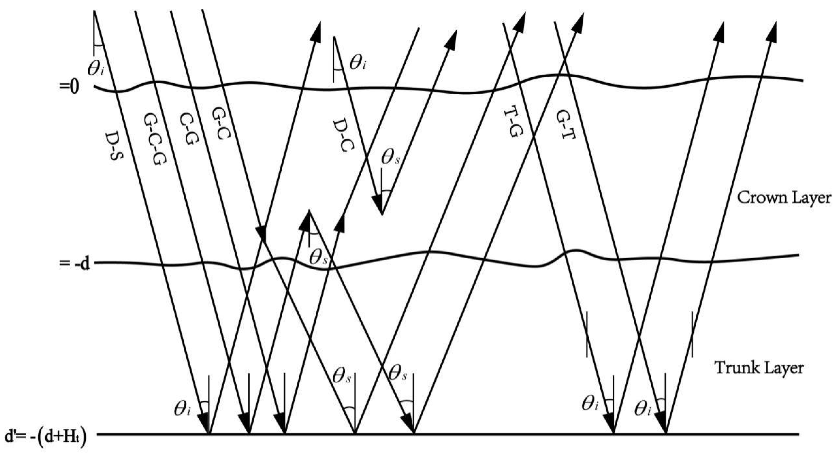
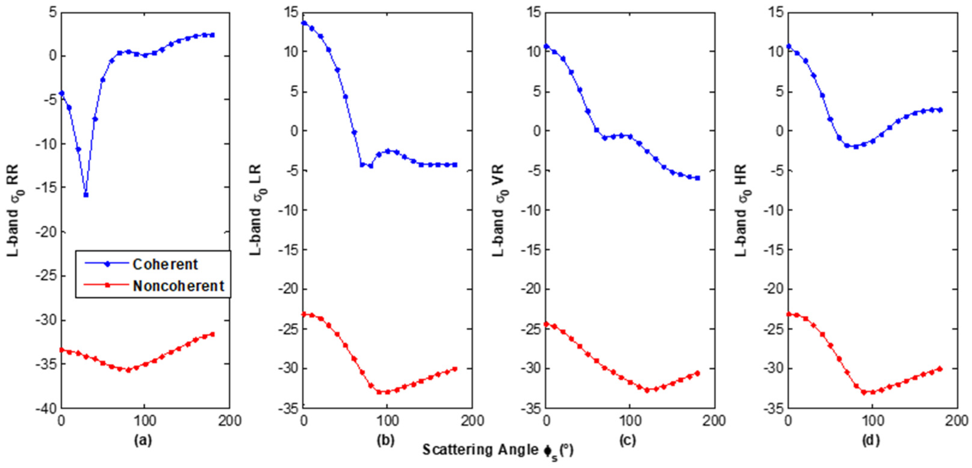
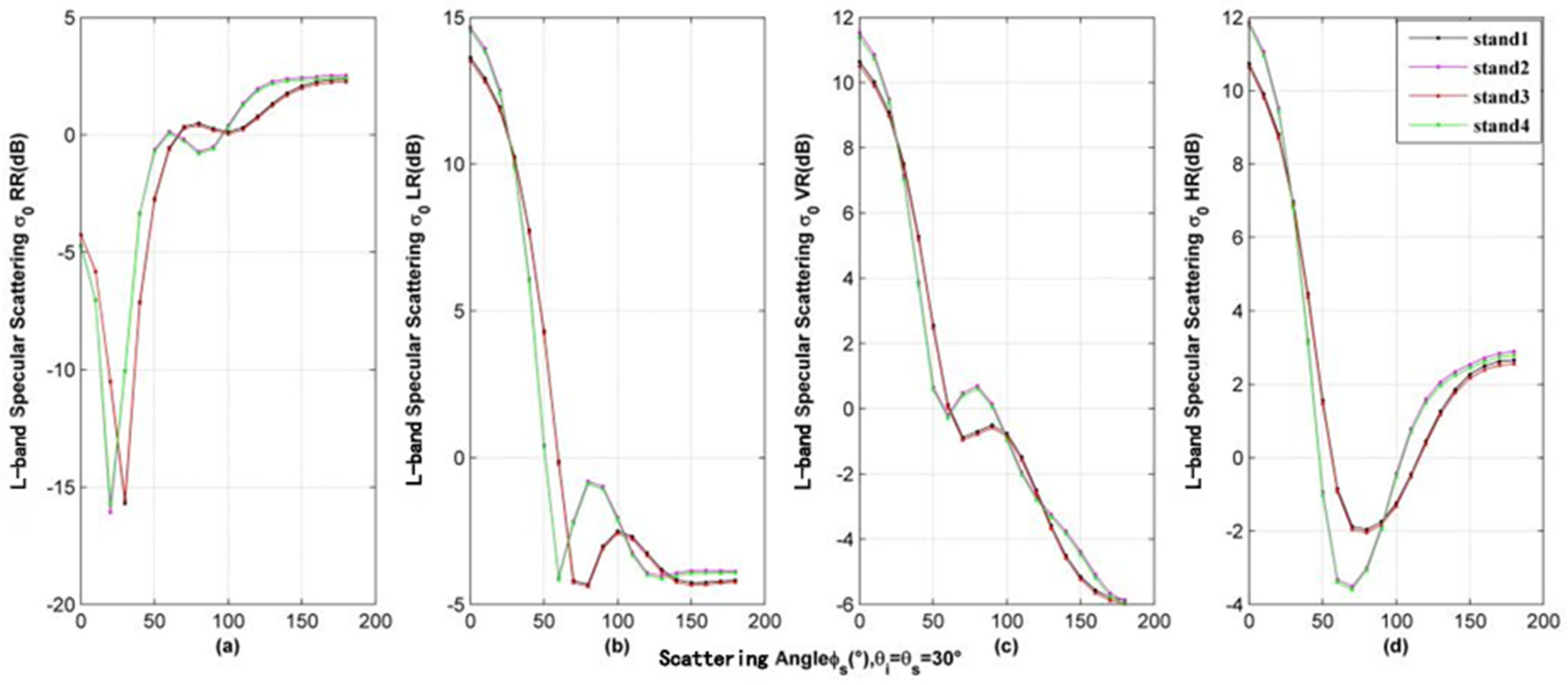
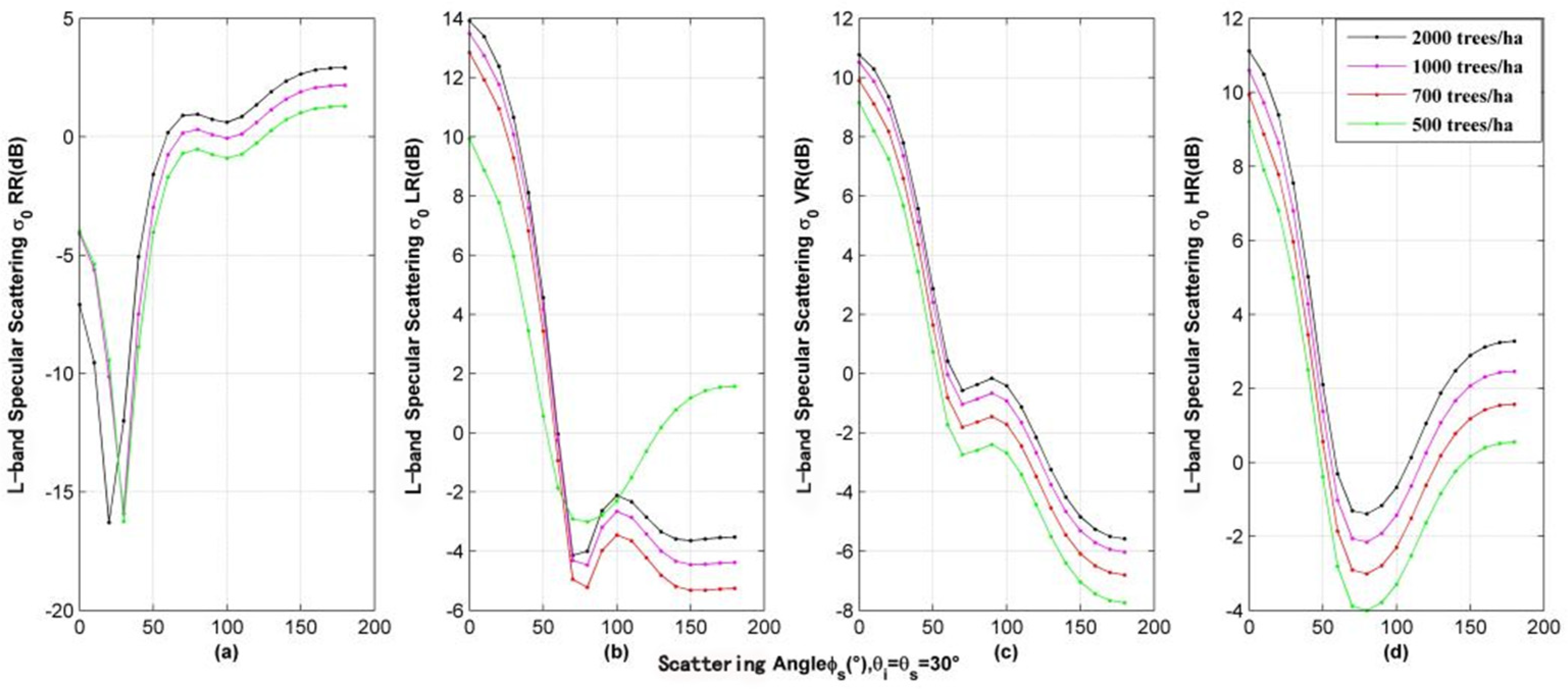
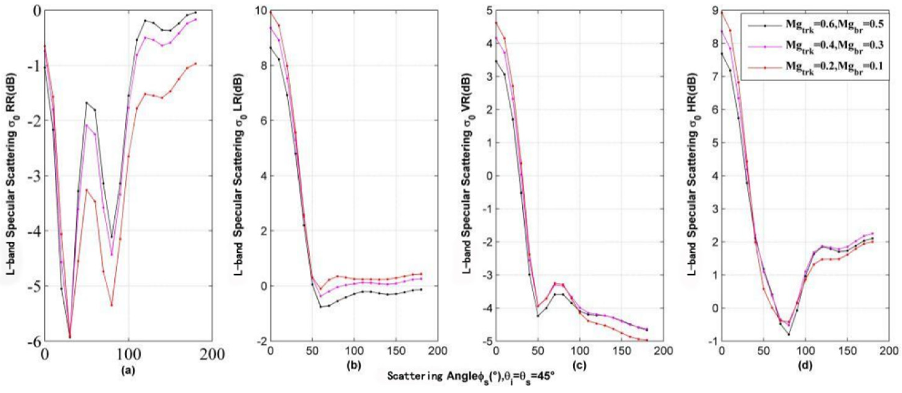
Wu et al. focused on using the vegetation first-order radiation transfer equation model to study the polarization characteristics of different canopies [51,52,53]. It is worth noting that the traditional first-order radiation transfer equation model mainly focuses on the linear polarization of monostatic-radar or radiometers to study the backscattering or radiation characteristics [54]. Wu et al. have employed its bistatic scattering and full-polarization characteristics to describe in more detail the bistatic scattering characteristics of different vegetation when the observation geometry and polarization characteristics change [51]. In their work, the polarization synthesis method is employed to calculate the scattering characteristics of various polarizations including circular polarization. When the transmitted signals are RHCP, the received signals are circular polarization (RHCP and LHCP) and linear polarization (horizontal polarization and vertical polarization), and the corresponding scattering characteristics are simulated. At the same time, the article also compares and analyzes the linear polarization scattering characteristics and the circular polarization scattering. The scattering difference in polarization puts forward a new direction of using polarization characteristics for GNSS-R land surface remote sensing monitoring. This is because the backscattering model has been verified by measured data, and the in-situ measurement data of bistatic radar limit the feasibility of its data verification. Therefore, the author verified the reliability of the developed model in the bistatic and full-polarization scattering characteristics through the method of “model verification model” [51,52,53]. However, actual measured data are still needed to verify the model in the near future.

3. Existing Problems

For the purpose of the final inversion application, this section will analyze and discuss the existing problems in the GNSS-R vegetation study.

3.1. Polarization Characteristics

Different from the traditional microwave remote sensing techniques, the GNSS-R employs the RHCP to overcome the ionospheric influence. Meanwhile, the polarization characteristics of the electromagnetic wave will change after the direct signal of the navigation satellite interacts with the vegetation parameters.

The GNSS-R technique is firstly applied to the ocean surface, which is more uniform than the land surface and the surface polarization characteristics are not obvious. As for the in-situ measurement and spaceborne missions, the LHCP polarized antenna is used for the collection of the reflected signals.

Early ground-based, airborne, and other land surface experiments have repeatedly tried to discover the difference in polarization characteristics. In the earliest SMEX02/03 airborne GPS-R experiment [55], it is believed that the reflected energy signal on the surface is mainly LHCP, so the RHCP antenna is used to receive the direct signal from the navigation satellite, and the LHCP is used to receive the reflected signal from the surface; meanwhile, the subsequent BAO (Boulder Atmospheric Observatory) tower experimental receiver uses RHCP to receive direct signals. In order to effectively use the reflected signals and reduce the impact of surface roughness on the accuracy of soil moisture inversion, a low-gain LHCP antenna and four high-gain LHCP, RHCP, H, and V polarized antennas are used to receive ground reflection signals [56]. In order to effectively use the Brewster angle and improve the inversion accuracy, the ground-based experiment of UPC University uses SMIGOL and PSMIGOL receivers, and the antenna adopts V polarization and H polarization [28]. The SAM receiver in the LEiMON experiment uses RHCP and LHCP antennas to receive ground reflection signals [57].

In terms of spaceborne, the receiver in SMAP-R is the radar in the SMAP satellite. Its receiver antenna uses the V and H linear polarizations; both TDS-1 and CYGNSS satellites use LHCP antenna to receive the reflected signal from the surface.

It can be seen from the above that the polarization of the receiver antenna is changing. There is no clear determinism to indicate which polarized receiver antenna is most beneficial for vegetation monitoring. Therefore, for the monitoring and retrieval of vegetation biomass, it is urgent to carry out research on the polarization characteristics of GNSS-R [51,53]. It is necessary to point out the difference in polarization from the theoretical mechanism level, and carry out the parameterized models based on polarization characteristics [58].

Vegetation shows different scattering characteristics to different polarization electromagnetic waves, and the scattering mechanism can be described by surface scattering, dihedral angle scattering, and volume scattering. Flat bare soil is prone to surface scattering, while large tree trunks and rough ground usually have dihedral angle scattering. Vegetation such as forest, crop, and shrub are easy to produce volume scattering. Wu et al. simulated and analyzed eight scattering mechanisms (including G-C-G (ground reflection and cross scattering and ground reflection), C-G (cross scanning and ground reflection), DC (direct cross bistatic scattering), G-C (ground reflection and cross scattering), and SG (the specific ground reflection)) [51]. Different scattering characteristics in different vegetation parameters and observed geometry and system parameters have also been simulated. These research results provide a certain theoretical support for the follow-up study of polarization GNSS-R remote sensing. In the traditional SAR remote sensing, there is a polarimetric SAR imaging system, and with the development of GNSS-R technology, the future polarimetric GNSS-R observation satellite also has potential feasibility. Polarization decomposition is an important technical means to reveal the scattering mechanism of ground objects. Polarization decomposition features play an important role in identifying the types of ground objects. GNSS-R’s unique combination of circular polarization and linear polarization will provide unique convenience for extracting vegetation parameter information using polarization decomposition technology. How to obtain the most polarized combination is an urgent problem to be solved in scattering mechanism research and data analysis in the future.

3.2. Utilization of Observation Angle for Vegetation Biomass Monitoring

A significant advantage of GNSS-R technology is multi-angle observation. Navigation satellites continuously emit direct signals, which are received at various angles, and the signals reflected by the ground surface can produce scattered signals at various scattering zenith angles and scattering azimuth angles. With the improvement and promotion of receiver performance, more of these scattered signals on the ground are likely to be received to a large extent in the future. The GNSS-R technology in ocean surface is relatively early, and the angle processing is usually normalized, that is, all incident angles are normalized to intermediate angles. Many studies on the land surface have followed this processing method [59,60]. However, its limitation is that GNSS-R has not exerted an effective practical value on the massive data obtained by multi-angle and omni-directional observation of ground objects. Due to the anisotropy of land surface parameters, there are obvious differences in the scattering characteristics at different angles. How to mine angle information, develop parameterized models suitable for different angles, and improve the inversion accuracy based on multi-angle information is an important aspect of GNSS-R for vegetation biomass monitoring.

3.3. Better Understanding of the Coherent and Incoherent Scattering of GNSS Signal

In most cases, the sea surface is in a non-stationary state. Affected by wind stress and swells propagating in the adjacent sea area, the sea surface roughness scale corresponding to the generated sea surface waves is much larger than the wavelength scale of the GNSS signal. Therefore, the GNSS signal mainly produces diffuse scattering on the sea surface. In the ocean applications of spaceborne GNSS-R, the discussion of the coherence of GNSS signals scattered from the sea surface is less discussed.

The GNSS signal scattering on the land surface is more complicated. In addition to being affected by the surface soil moisture, the scattering signal will also be affected by the surface roughness, vegetation, terrain, soil texture, and inland water bodies. The incident GNSS signal usually undergoes coherent and noncoherent scattering on the actual land surface. There are several works [61,62] concentrated on this topic. However, the analysis of spaceborne data (CYGNSS and TDS-1) mostly thinks that the received energy is mainly coherent scattering, and the simulation analysis of the theoretical model also points out that the coherent scattering energy is larger than the incoherent scattering energy [63]. In GNSS-R, coherent and incoherent observations have different surface scattering mechanisms. This difference is mainly manifested in the power extension and magnitude difference of the observed DDM. A coherent DDM is closer to the WAF (Woodward Ambiguity Function) of the GNSS navigation signal itself, while a noncoherent DDM has very obvious power spread characteristics in terms of delay and Doppler [64].

The articles [65,66] propose a classification method to determine the coherence of CYGNSS 454 terrestrial observation DDM. Since the GNSS signals received by the satellite receiver from the non-calm sea surface are all non-coherent signals, the power distribution of the coherent DDM received from the flat surface is close to the WAF. According to the power spread and magnitude characteristics of typical coherent and noncoherent DDM, six classification estimators are established to identify the coherence of CYGNSS terrestrial DDM. The classification results show that when the estimator based on the DDM absolute scattering power feature is used, it is more difficult to distinguish the coherence of the DDM and the estimator that characterizes the power spread feature can better separate the coherent and incoherent DDM [65,66]. In the future, how to combine the scattering physical mechanism (especially microwave scattering mechanism) and signal explanation to fully utilize the coherent and noncoherent signals together should be paid much more attention.

3.4. Improve Our Understanding of the Mechanism Model for Vegetation

The goal of a GNSS-R/GNSS-IR model for vegetation is to establish the relationship between surface vegetation parameters and the GNSS reflection signal. That is to establish the relationship between vegetation parameters, observation geometric parameters, and delay Doppler diagram or multi-path observables (SNR, phase, and pseudo-range). Although the N-L multi-path forward GPS model can simulate the influence of vegetation parameters on multi-path signals, the premise is that the receiver can only receive the specular reflection energy of vegetation in the First Fresnel Zone (FFZ). However, several works published recently have pointed out that the noncoherent energy coming from the outside of FFZ should not be ignored during the calculations [61,62].

When calculating the scattering characteristics of vegetation, the dielectric constant of the vegetation is input into the circular polarization reflection coefficient, and information such as the antenna model, observation geometry, and system parameters are coupled, and finally, SNR, phase, and pseudo-range information are obtained. The calculation of the vegetation scattering characteristics in the model is without considering incoherent scattering, and at the same time, it is unable to simulate the scattering, reflection, and attenuation information of the navigation satellite signal in the vegetation layer. Most of the existing microwave scattering models are for monostatic radar backscattering models or emissivity models for radiometers, and there are relatively few bistatic scattering models for GNSS-R. In addition, the polarization considerations in the existing models are lacking. The subsequent models need to consider the characteristics of circular polarization and the scattering capabilities of different polarizations combined with circular polarization and linear polarization. Only the model that has this function can effectively analyze and mine the polarization characteristics, carry out the inversion of the relevant vegetation biomass according to its polarization characteristics information, and use the polarization information to improve the accuracy of the inversion [51,52,53].

Accurately understanding and describing the microwave scattering mechanism of rough surfaces and vegetation parameters is the most important theoretical basis for GNSS-R surface parameter remote sensing. It can be used for the analysis and interpretation of satellite observations, satellite data simulation, and satellite data assimilation. Theoretical models can also be employed for the development of quantitative surface parameters’ retrieval algorithms, and they are the key mechanism tools for new sensor design [67]. Therefore, we must vigorously promote and strengthen the research on GNSS-R remote sensing theoretical modeling in the follow-up study.

4. Model Simulations and Discussion

As for the spaceborne GNSS-R vegetation study, the existing research is mostly based on observational data to establish the sensitivity analysis. It is generally in the research stage of qualitative analysis and lacks the discovery of the physical mechanism behind it. Since GNSS-R is a bistatic radar with separate transceivers, the existing microwave scattering models for monostatic radars or radiometers are no longer applicable.

Therefore, it is necessary to improve the traditional backscattering and emissivity models to obtain a microwave scattering mechanism model suitable for GNSS-R. According to the existing problems in GNSS-R vegetation remote sensing, this part will combine the previous developed microwave vegetation scattering models to analyze its scattering characteristics and discuss the future development trends [51,52,53,54]. Some basic information of the employed models is provided in Section 4.1. While more detailed information of the model is given in the literature [54], it is worth mentioning that although there are many theoretical simulators as presented in Section 2.4, fewer works give detailed comparisons of vegetation parameters (such as vegetation density, water content, etc.) on the bistatic scattering properties at various polarizations. While the bistatic scattering properties provide the basic information for parameters retrieval, they need to pay more attention to simulations; therefore, we will give more details on the simulations in this section. We will also give a brief introduction to the model we used in GNSS-R.

4.1. Theoretical Models

The Bi-MIMICS (Bitstaic-Michigan Microwave Canopy Scattering Model) model is based on the first-order solution of the radiative transfer equation. In the model, the forest stand is divided into canopy layer, trunk layer, and rough surface layer (Figure 1). The first-order scattering includes the single scattering of each layer and double scattering between layers. The canopy is simulated as a dielectric cylinder (representing needles or branches) and a disc (representing leaves). The trunk layer is composed of a uniform radius of perpendicularly facing dielectric cylinders. Regarding the circular polarization characteristics of GNSS-R, the Bi-MIMICS model needs to be modified by the method of polarization synthesis, so that it can calculate the scattering characteristics of any polarization. The improved model can calculate the scattering characteristics of any polarization under any observation geometry [48]. There are eight scattering mechanisms in the model: G-C-G, C-G, DC, G-C, G-T, DG, T-G, and the S-G.

Traditional microwave electromagnetic scattering models or radiation models are mainly aimed at the linear polarization characteristics of radars or radiometers. Therefore, the traditional models pay less attention to the circular polarization characteristics. In order to overcome the impact of the ionosphere, GNSS satellites emit signals in RHCP polarization. After this kind of signal is reflected on the ground, the polarization characteristics will change. Therefore, if we conduct research on GNSS-R, it is necessary to improve the traditional model so that it can calculate the scattering characteristics of various polarizations. Regarding the first-order radiation transfer equation model used in this paper, the wave synthesis technique is used to modify the model. It should be noted that before the wave synthesis technique is used, a 4 × 4 transformation matrix is needed to be constructed in the model. The corresponding formula of the wave synthesis technique is like the following:

$${\sigma }_r{}_t({\psi }_r,{\chi }_r,{\psi }_t,{\chi }_t)=4\pi {\tilde{Y}}_m^r{M}_m{Y}_m^t$$

(1)

where $M_m$ is the first-order fully polarized transformation matrix, i.e., the normalized Mueller matrix. ${\tilde{Y}}_m^r$ ${\mathrm{Y}}_{\mathrm{m}}^r$ and $Y_m^t$ are the normalized Stokes vectors characterizing the transmitter and receiver polarization. By using this technique, we can obtain the bistatic scattering cross section ${\sigma }_r{}_t$ for any combination of transmit and receive polarizations. The subscript r and t represent the polarization of receiver and transmitter, respectively. As can be seen from Equation (1), the final bistatic scattering cross section is a function of the orientation and ellipticity angles ($\psi$ and $\chi$), as shown in Figure 2.

The two angles $\psi$ and $\chi$ are sufficient to specify the polarization completely. The normalized Stokes vectors can be represented like the following:

$$Y_m=\left[\begin{array}{c}\frac{1}{2}\left(1+\cos 2\psi \cos 2\chi \right)\\ \frac{1}{2}(1-\cos 2\psi \cos 2\chi )\\ \sin 2\psi \cos 2\chi \\ \sin 2\chi \end{array}\right]$$

(2)

Table 1. Modified Stokes vectors for various polarizations.

	V Pol	H Pol	LHCP Pol	RHCP Pol	+45° Pol	−45° Pol
Modified Stokes vector	$\left[\begin{array}{c}1\\ 0\\ 0\\ 0\end{array}\right]$	$\left[\begin{array}{c}0\\ 1\\ 0\\ 0\end{array}\right]$	$\left[\begin{array}{c}0.5\\ 0.5\\ 0\\ 1\end{array}\right]$	$\left[\begin{array}{c}0.5\\ 0.5\\ 0\\ -1\end{array}\right]$	$\left[\begin{array}{c}0.5\\ 0.5\\ -1\\ 0\end{array}\right]$	$\left[\begin{array}{c}0.5\\ 0.5\\ 1\\ 0\end{array}\right]$

presents the modified Stokes vectors corresponding to several commonly used polarizations.

During our simulations in Section 4.4, we employed Aspen as a representative. The detail input parameters are shown in

Table 2. Model inputs for the MIMICS model.

Stand	Aspen
Trunk density (number/ha)	1100
Trunk height (m)	8
Trunk diameter (cm)	24
Trunk moisture (gravimetric)	0.5
Crown depth (m)	2
Brunch density (number/m3)	4.1
Branch length (m)	0.75
Branch diameter (cm)	0.7
Branch moisture (gravimetric)	0.4

and

Table 3. The permittivity of soil and canopy layers.

Stand	Soil	Trunk	Branch
Aspen	5.99 + 0.99 i	14.49 + 4.76 i	10.19 + 3.36 i

.

4.2. Polarization Difference

When the incident signal polarization is RHCP and the received signal is circular polarization and linear polarization, the coherent (${\mathsf{\theta }}_{\mathrm{i}}={\mathsf{\theta }}_{\mathrm{s}},{\mathsf{\phi }}_{\mathrm{s}}=0^{°}$) and incoherent (${\mathsf{\theta }}_{\mathrm{i}}={30}^{°},{\mathsf{\phi }}_{\mathrm{s}}={120}^{°}$) scattering properties are shown in Figure 1. Here ${\mathsf{\theta }}_{\mathrm{i}}$ is the incidence angle, ${\mathsf{\theta }}_{\mathrm{s}}$ is the scattering zenith angle, while ${\mathsf{\phi }}_{\mathrm{s}}$ is the scattering azimuth angle. As most of the frequency bands of the present GNSS constellations cover the lower L-band to upper L-band, and the scattering properties at these bands are almost the same, we select GPS L1 band for the following simulations. For the same polarization, the energy value of coherent scattering (Figure 3a) is significantly greater than that of incoherent scattering (Figure 3b). For the same kind of ground objects under the same observation geometry, when the polarization characteristics change, the corresponding microwave scattering characteristics also have obvious differences (Figure 1). The difference in the scattering characteristics of different polarizations is related to the observation geometry. When the angle is different, the scattering properties of the various polarizations are different. It is worth noting that the VR polarization has a scattering groove in the simulated angle range (Figure 3a), which is mainly caused by the Brewster angle. Figure 3b has a scattering peak at thetas = 30°, which is mainly caused by the strong scattering of the tree trunk.

It can be seen from the simulation in Figure 3 that the scattering characteristics of vegetation at different polarizations are significantly different, so how to effectively use polarization information in vegetation monitoring is an important content of subsequent development.

4.3. Differences in Coherent and Incoherent Scattering Characteristics

Figure 4 shows the comparison between coherent scattering (${\mathsf{\theta }}_{\mathrm{i}}={30}^{\circ }$, ${\mathsf{\theta }}_{\mathrm{s}}=30^{\circ }$, ${\mathsf{\phi }}_{\mathrm{s}}=0^{\circ }~{180}^{\circ }$) and noncoherent scattering (${\mathsf{\theta }}_{\mathrm{i}}={10}^{\circ }$, ${\mathsf{\theta }}_{\mathrm{s}}=50^{\circ }$, ${\mathsf{\phi }}_{\mathrm{s}}=0^{\circ }~{180}^{\circ }$). The simulation analysis shows that the energy of coherent scattering is much larger than that of incoherent scattering at various polarizations. At present, when using CYGNSS data to study vegetation parameters, it is basically considered that the energy of the receiver is coherent scattering energy. In the later application process, how to effectively extract incoherent scattering energy and use this part of the information to obtain more vegetation information will be a direction of future development.

4.4. The Influence of Observation Geometry on Scattering Characteristics

Figure 3a shows the relationship between the scattering characteristics and the specular scattering angle, and Figure 3b shows the relationship between the scattering characteristics and the scattering zenith angle, while the incident angle (${\mathsf{\theta }}_{\mathrm{i}}={30}^{°}$) and scattering azimuth angle (${\mathsf{\phi }}_{\mathrm{s}}={120}^{°}$) are fixed. It can be seen that in different observation geometries, the scattering characteristics corresponding to various polarizations are obviously different. Figure 4 shows that in various polarizations, the scattering difference corresponding to the scattering azimuth angle also changes significantly. However, angle information is not well used in GNSS-R vegetation and soil moisture remote sensing. The normalization of angles or simple angle intervals for the characteristic analysis greatly limits the unique advantages of angle observation in GNSS-R. Due to the anisotropy of vegetation, how to effectively use its scattering characteristics under different observation angles to find the optimal observation geometry is a problem faced by GNSS-R vegetation remote sensing.

4.5. Different Vegetation Parameters at Various Polarizations on the Scattering Characteristics

Whether the vegetation parameters (such as water content and biomass, etc.) can be quantitatively analyzed using GNSS-R is a problem that needs to be solved in the later development of GNSS-R. Based on the observation geometry and polarization characteristics, the corresponding scattering properties (L-band) of different vegetation parameters will be analyzed in this section.

Table 4. Diameters of Aspen stands.

	Stand 1	Stand 2	Stand 3	Stand 4
Trunk diameter (cm)	24	30	24	30
Branch diameter (cm)	0.7	0.7	0.9	0.9

shows the trunk and branch diameters of four stands.

Figure 5 shows the scattering characteristics of various polarizations in the specular scattering. The four stands have different diameters. It can be seen that when the trunk diameter changes, the corresponding scattering characteristics are significantly different. However, the change in the branch diameters has little effect on the scattering characteristics. It is known that the trunk diameter has the most obvious impact on the forest biomass. How to use the GNSS-R receiver terminal signal to effectively separate the forest biomass and use this remote sensing technology to monitor the forest biomass is one of the future development directions.

As for different canopy densities (as shown in

Table 5. Tree density for four different forest scenarios.

	Forest 1 (Trees/ha)	Forest 2 (Trees/ha)	Forest 3 (Trees/ha)	Forest 4 (Trees/ha)
Tree density	2000	1000	700	500

), Figure 6 shows the corresponding specular scattering characteristics of various polarizations. Under the above observation geometry, it can be seen from the simulation results in Figure 6 that when the canopy density is different, the scattering characteristics are significantly different. Whether the GNSS-R signal caused by the difference in canopy density can be effectively monitored, and the use of this technology to conduct remote sensing research on vegetation density-related information will be a problem to be solved in the future.

Figure 7 shows the specular scattering characteristics of different vegetation water contents (

Table 6. Vegetation water content and permittivity for the three scenarios.

	Trunk		Branch
	Moisture	Permittivity	Moisture	Permittivity
Aspen1	0.6	41.84 + 18.93 i	0.5	32.97 + 14.73 i
Aspen2	0.4	25.60 + 11.25 i	0.3	19.29 + 8.28 i
Aspen3	0.2	13.33 + 5.47 i	0.1	6.67 + 2.33 i

). For different vegetation water contents, we have employed the vegetation dielectric constant model to calculate its permittivity. The moisture contents of the vegetation scatterer (trunk and branch) are from very high content to low content. It can be seen from the simulation results that when the vegetation water content changes, the corresponding specular scattering characteristics are different. Whether GNSS-R can be used to effectively detect or invert vegetation water content information will be a technical issue that needs to be broken through in future development.

This section has given the bistatic scattering responses corresponding to different vegetation geophysical parameters and observation geometry at various polarizations. From the simulations (Figure 3, Figure 4, Figure 5, Figure 6 and Figure 7), we can see that as the polarization and scattering geometry change (the same geophysical parameters set constants), there are obvious bistatic scattering properties (Figure 3 and Figure 4). However, as the above two variables set constants for different vegetation parameters (Figure 5, Figure 6 and Figure 7), the bistatic scattering properties almost keep the same for some cases, and have apparent changes for other cases, which are related to the observation geometries and polarizations. Therefore, if we well utilize the geometry and polarization, then the vegetation parameters have the potential to be detected. In other words, if we ignore or take less consideration of the information of observation geometry and polarization, it is hard to detect.

Given the importance of observation geometry and polarizations for the final vegetation parameters’ detection, we need the corresponding measurement data to validate this information. However, due to the limits of the present in-situ campaigns, we cannot find abundant data to back up this assumption. We have to ask for the theoretical model and the corresponding simulations for help.

4.6. Development of Retrieval Algorithm

The ultimate goal of remote sensing development is to achieve an efficient and convenient inversion algorithm. GNSS-R technology, especially spaceborne GNSS-R technology, is feasible in vegetation monitoring, but there is still a certain gap to the quantitative inversion of vegetation parameters. The development and use of an efficient and convenient inversion algorithm will make this technology truly practical in vegetation remote sensing and it is an inevitable development trend in the future. According to the above simulation of the difference in scattering characteristics, it can be seen that when the vegetation parameters (vegetation water content, density, and height) change under different polarizations and different observation angles, the scattering characteristics are different. How to effectively identify and reverse the information in the receiver signal is one of the challenges. There is a complex nonlinear relationship between GNSS-R observations and vegetation parameters. At present, it is relatively easy to use machine learning such as neural networks to invert forest parameters [36] because machine learning can model the nonlinear relationship well and achieve relatively good inversion accuracy.

The later development of inversion algorithms can cover but is not limited to empirical models based on optimization theoretical algorithms and semi-empirical inversion models simplified based on theoretical models. The empirical model can create a function based on the statistical analysis of ground measurement data and ground object parameters. This function mainly describes the function fitting relationship between GNSS-R observations and ground object parameters. The semi-empirical inversion model comes from the simplification of the theoretical model. The measured data are used to partially fit the theoretical model coefficients, which reduce the amount of calculation tasks and complexity, and then a definite analytical solution can be obtained.

5. Conclusions

GNSS-R technology is an emerging method of Earth observation that uses the reflected signals of navigation satellites for remotely sensing terrestrial objects. Compared with the ocean applications, the research in the field of terrestrial remote sensing using GNSS-R is relatively lagging. The research on vegetation parameters using spaceborne GNSS-R technology is still in the exploratory research stage. Existing research is mostly based on a qualitative analysis and the analysis is dependent on the spaceborne observation data. In this paper, we reviewed the current research status, and then the microwave scattering model was employed to analyze the effects of coherent and incoherent scattering, polarization, different vegetation parameters, and observation geometry on the final scattering characteristics. It points out the potential research direction of this technology and the technical bottleneck that urgently needs to be broken through. How to use the scattering characteristics under different observation geometries and polarizations to determine the optimal observation combination (observation geometry and polarization) and develop the quantitative retrieval methods will be the key research directions for future development. The specific prospects that can improve the vegetation retrieval using GNSS-R should be paid attention to and can be summarized into two items.

The first one is how to fully dig the observation geometry information in DDM. As we know, several works have pointed out that the noncoherent scattering properties should not be ignored and the information outside the specular direction can be employed to get more information on the vegetation parameters. However, the main difficulty for this is that the angle information is all integrated and the information from different angles is coupled in a DDM waveform. Then, how to use the DDM information from different scattering azimuth angles and zenith angles can be studied in the near future.

The second item is that the polarization information of vegetation should be paid extra attention, since most of the present works lack the mining of polarization information. However, the vegetation will show specific different properties at various polarizations. Therefore, in the future, how to fully use the polarization information to get the vegetation properties should be one key direction that needs to be solved.

References

1. Hall, C.D.; Cordey, R.A. Multistatic Scatterometry. In Proceedings of the International Geoscience and Remote Sensing Symposium, ‘Remote Sensing: Moving Toward the 21st Century’, Edinburgh, UK, 12–16 September 1988. [Google Scholar]
2. Martin-Neira, M.A. Passive Reflectometry and Interferometry System (PARIS): Application to ocean altimetry. ESA J. 1993, 17, 331–355. [Google Scholar]
3. Zavorotny, V.U.; Gleason, S.; Cardellach, E.; Camps, A. Tutorial on Remote Sensing Using GNSS Bistatic Radar of Opportunity. IEEE Geosci. Remote Sens. Mag. 2014, 2, 8–45. [Google Scholar] [CrossRef] [Green Version]
4. Gleason, S.; Adjrad, M.; Unwin, M. Sensing ocean, ice and land reflected signals from space: Results from the UK-DMC GPS reflectometry experiment. In Proceedings of the 18th International Technical Meeting of the Satellite Division of The Institute of Navigation, Palm Springs, CA, USA, 1 January 2005; pp. 1679–1685. [Google Scholar]
5. Ruf, C.S.; Chew, C.; Lang, T.; Morris, M.G.; Nave, K.; Ridley, A.; Balasubramaniam, R. A New Paradigm in Earth Environmental Monitoring with the CYGNSS Small Satellite Constellation. Sci. Rep. 2018, 8, 8782. [Google Scholar] [CrossRef] [Green Version]
6. Li, W.; Cardellach, E.; Fabra, F.; Rius, A.; Ribó, S.; Martín-Neira, M. First spaceborne phase altimetry over sea ice using TechDemoSat-1 GNSS-R signals. Geophys. Res. Lett. 2017, 44, 8369–8376. [Google Scholar] [CrossRef]
7. Mayers, D.; Ruf, C. Tropical Cyclone Center Fix Using CYGNSS Winds. J. Appl. Meteorol. Clim. 2019, 58, 1993–2003. [Google Scholar] [CrossRef]
8. Warnock, A.; Ruf, C. Response to Variations in River Flowrate by a Spaceborne GNSS-R River Width Estimator. Remote Sens. 2019, 11, 2450. [Google Scholar] [CrossRef] [Green Version]
9. Morris, M.; Chew, C.; Reager, J.T.; Shah, R.; Zuffada, C. A novel approach to monitoring wetland dynamics using CYGNSS: Everglades case study. Remote Sens. Environ. 2019, 233, 111417. [Google Scholar] [CrossRef]
10. Chew, C.; Reager, J.T.; Small, E. CYGNSS data map flood inundation during the 2017 Atlantic hurricane season. Sci. Rep. 2018, 8, 9336. [Google Scholar] [CrossRef] [PubMed]
11. Sun, Y.; Liu, C.; Du, Q. Global navigation satellite system occultation sounder II (GNOS II). In Proceedings of the 2017 IEEE International Geoscience and Remote Sensing Symposium (IGARSS), Fort Worth, TX, USA, 23–28 July 2017; pp. 1189–1192. [Google Scholar]
12. Munoz-Martin, J.; Llaveria, D.; Herbert, C.; Pablos, M.; Park, H.; Camps, A. Soil Moisture Estimation Synergy Using GNSS-R and L-Band Microwave Radiometry Data from FSSCat/FMPL-2. Remote Sens. 2021, 13, 994. [Google Scholar] [CrossRef]
13. Unwin, M.J.; Pierdicca, N.; Cardellach, E.; Rautiainen, K.; Foti, G.; Blunt, P.; Guerriero, L.; Santi, E.; Tossaint, M. An Introduction to the HydroGNSS GNSS Reflectometry Remote Sensing Mission. IEEE J. Sel. Top. Appl. Earth Obs. Remote Sens. 2021, 99, 1. [Google Scholar]
14. Kerr, Y.H.; Waldteufel, P.; Wigneron, J.-P.; Delwart, S.; Cabot, F.; Boutin, J.; Escorihuela, M.J.; Font, J.; Reul, N.; Gruhier, C.; et al. The SMOS Mission: New Tool for Monitoring Key Elements ofthe Global Water Cycle. Proc. IEEE 2010, 98, 666–687. [Google Scholar] [CrossRef] [Green Version]
15. Entekhabi, D.; Njoku, E.G.; O’Neill, P.; Kellogg, K.H.; Crow, W.; Edelstein, W.N.; Entin, J.K.; Goodman, S.D.; Jackson, T.J.; Johnson, J.; et al. The Soil Moisture Active Passive (SMAP) Mission. Proc. IEEE 2010, 98, 704–716. [Google Scholar] [CrossRef]
16. Chew, C.; Small, E. Estimating inundation extent using CYGNSS data: A conceptual modeling study. Remote Sens. Environ. 2020, 246, 111869. [Google Scholar] [CrossRef]
17. Kim, H.; Lakshmi, V. Use of Cyclone Global Navigation Satellite System (CyGNSS) Observations for Estimation of Soil Moisture. Geophys. Res. Lett. 2018, 45, 8272–8282. [Google Scholar] [CrossRef] [Green Version]
18. Clarizia, M.P.; Pierdicca, N.; Costantini, F. Analysis of CYGNSS data for soil moisture retrieval. IEEE J. Sel. Top. Appl. Earth Obs. Remote Sens. 2019, 12, 2227–2235. [Google Scholar] [CrossRef]
19. Al-Khaldi, M.M.; Johnson, J.T.; O’Brien, A.J.; Balenzano, A.; Mattia, F. Time-Series Retrieval of Soil Moisture Using CYGNSS. IEEE Trans. Geosci. Remote Sens. 2019, 57, 4322–4331. [Google Scholar] [CrossRef]
20. Yan, Q.; Huang, W.; Jin, S.; Jia, Y. Pan-tropical soil moisture mapping based on a three-layer model from CYGNSS GNSS-R data. Remote Sens. Environ. 2020, 247, 111944. [Google Scholar] [CrossRef]
21. Camps, A.; Vall·llossera, M.; Park, H.; Portal, G.; Rossato, L. Sensitivity of TDS-1 GNSS-R Reflectivity to Soil Moisture: Global and Regional Differences and Impact of Different Spatial Scales. Remote Sens. 2018, 10, 1856. [Google Scholar] [CrossRef] [Green Version]
22. Ferrazzoli, P.; Guerriero, L.; Pierdicca, N.; Rahmoune, R. Forest biomass monitoring with GNSS-R: Theoretical simulations. Adv. Space Res. 2011, 47, 1823–1832. [Google Scholar] [CrossRef]
23. Loria, E.; O’Brien, A.; Zavorotny, V.; Lavalle, M.; Chew, C.; Shah, R.; Zuffada, C. Analysis of Wetland Extent Retrieval Accuracy Using CYGNSS. In Proceedings of the IGARSS 2019–2019 IEEE International Geoscience and Remote Sensing Symposium 2019, Yokohama, Japan, 28 July–2 August 2019. [Google Scholar]
24. Haase, J.S.; Xie, F.; Muradyan, P.; Garrison, J.L.; Lulich, T.; Voo, J.; Larson, K.M. New Atmospheric Observations from the Airborne GNSS Instrument System for Multistatic and Occultation Sensing (GISMOS). In Proceedings of the AGU Fall Meeting Abstracts 2008, San Francisco, CA, USA, 15–19 December 2008. [Google Scholar]
25. Chew, C.; Small, E.E.; Larson, K.M. An algorithm for soil moisture estimation using GPS-interferometric reflectometry for bare and vegetated soil. GPS Solutions 2015, 20, 525–537. [Google Scholar] [CrossRef]
26. Rodriguez-Alvarez, N.; Bosch, X.; Camps, A.; Ramos-Perez, I.; Valencia, E.; Park, H.; Vall-Llossera, M. Vegetation Water Content Estimation Using GNSS Measurements. IEEE Geosci. Remote Sens. Lett. 2011, 9, 282–286. [Google Scholar] [CrossRef]
27. Rodriguez-Alvarez, N.; Camps, A.; Vall-Llossera, M.; Bosch, X.; Monerris, A.; Ramos-Perez, I.; Valencia, E.; Marchan-Hernandez, J.F.; Martínez-Fernández, J.; Baroncini-Turricchia, G.; et al. Land Geophysical Parameters Retrieval Using the Interference Pattern GNSS-R Technique. IEEE Trans. Geosci. Remote Sens. 2010, 49, 71–84. [Google Scholar] [CrossRef]
28. Arroyo, A.A.; Camps, A.; Aguasca, A.; Forte, G.; Monerris, A.; Rüdiger, C.; Walker, J.P.; Park, H.; Pascual, D.; Onrubia, R. Improving the Accuracy of Soil Moisture Retrievals Using the Phase Difference of the Dual-Polarization GNSS-R Interference Patterns. IEEE Geosci. Remote Sens. Lett. 2014, 11, 2090–2094. [Google Scholar] [CrossRef] [Green Version]
29. Egido, A.E. GNSS Reflectometry for Land Remote Sensing Applications; Universitat Politècnica de Catalunya: Barcelona, Spain, 2014. [Google Scholar]
30. Carreno-Luengo, H.; Camps, A.; Querol, J.; Forte, G. First Results of a GNSS-R Experiment from a Stratospheric Balloon Over Boreal Forests. IEEE Trans. Geosci. Remote Sens. 2015, 54, 2652–2663. [Google Scholar] [CrossRef] [Green Version]
31. Egido, A.; Caparrini, M.; Ruffini, G.; Paloscia, S.; Santi, E.; Guerriero, L.; Pierdicca, N.; Floury, N. Global Navigation Satellite Systems Reflectometry as a Remote Sensing Tool for Agriculture. Remote Sens. 2012, 4, 2356–2372. [Google Scholar] [CrossRef] [Green Version]
32. Egido, A.; Paloscia, S.; Motte, E.; Guerriero, L.; Pierdicca, N.; Caparrini, M.; Santi, E.; Fontanelli, G.; Floury, N. Airborne GNSS-R Polarimetric Measurements for Soil Moisture and Above-Ground Biomass Estimation. IEEE J. Sel. Top. Appl. Earth Obs. Remote Sens. 2014, 7, 1522–1532. [Google Scholar] [CrossRef]
33. Zribi, M.; Guyon, D.; Motte, E.; Dayau, S.; Wigneron, J.P.; Baghdadi, N.; Pierdicca, N. Performance of GNSS-R GLORI data for biomass estimation over the Landes forest. Int. J. Appl. Earth Obs. Geoinf. 2018, 74, 150–158. [Google Scholar] [CrossRef]
34. Camps, A.; Park, H.; Pablos, M. Sensitivity of GNSS-R spaceborne observations to soil moisture and vegetation. IEEE J. Sel. Top. Appl. Earth Obs. Remote Sens. 2016, 9, 4730–4742. [Google Scholar] [CrossRef] [Green Version]
35. Carreno-Luengo, H.; Lowe, S.; Zuffada, C.; Esterhuizen, S.; Oveisgharan, S. Spaceborne GNSS-R from the SMAP Mission: First Assessment of Polarimetric Scatterometry over Land and Cryosphere. Remote Sens. 2017, 9, 362. [Google Scholar] [CrossRef] [Green Version]
36. Carreno-Luengo, H.; Luzi, G.; Crosetto, M. Above-Ground Biomass Retrieval over Tropical Forests: A Novel GNSS-R Approach with CyGNSS. Remote Sens. 2020, 12, 1368. [Google Scholar] [CrossRef]
37. Santi, E.; Paloscia, S.; Pettinato, S. Remote sensing of forest biomass using GNSS reflectometry. IEEE J. Sel. Top. Appl. Earth Obs. Remote Sens. 2020, 13, 2351–2368. [Google Scholar] [CrossRef]
38. Zavorotny, V.; Voronovich, A. Scattering of GPS signals from the ocean with wind remote sensing application. IEEE Trans. Geosci. Remote Sens. 2000, 38, 951–964. [Google Scholar] [CrossRef] [Green Version]
39. Nievinski, F.G.; Larson, K.M. Forward modeling of GPS multipath for near-surface reflectometry and positioning applications. GPS Solut. 2013, 18, 309–322. [Google Scholar] [CrossRef]
40. Larson, K.M. GPS interferometric reflectometry: Applications to surface soil moisture, snow depth, and vegetation water content in the western United States. Wiley Interdiscip. Rev. Water 2016, 3, 775–787. [Google Scholar] [CrossRef]
41. Chew, C.C.; Small, E.E.; Larson, K.M. Effects of Near-Surface Soil Moisture on GPS SNR Data: Development of a Retrieval Algorithm for Soil Moisture. IEEE Trans. Geosci. Remote Sens. 2014, 52, 537–543. [Google Scholar] [CrossRef]
42. Mccreight, J.L.; Small, E.E.; Larson, K.M. Snow depth, density, and SWE estimates derived from GPS reflection data: Validation in the western U.S. Water Resour. Res. 2015, 50, 6892–6909. [Google Scholar] [CrossRef]
43. Chew, C.C.; Small, E.E.; Larson, K.M.; Zavorotny, V.U. Vegetation Sensing Using GPS-Interferometric Reflectometry: Theoretical Effects of Canopy Parameters on Signal-to-Noise Ratio Data. IEEE Trans. Geosci. Remote Sens. 2015, 53, 2755–2764. [Google Scholar] [CrossRef]
44. Masters, D.S. Surface Remote Sensing Applications of GNSS Bistatic Radar: Soil Moisture and Aircraft Altimetry; University of Colorado: Boulder, CO, USA, 2004. [Google Scholar]
45. Pierdicca, N.; Guerriero, L.; Giusto, R.; Brogioni, M.; Egido, A. SAVERS: A Simulator of GNSS Reflections from Bare and Vegetated Soils. IEEE Trans. Geosci. Remote Sens. 2014, 52, 6542–6554. [Google Scholar] [CrossRef]
46. Kurum, M.; Deshpande, M.; Joseph, A.T.; O’Neill, P.E.; Lang, R.H.; Eroglu, O. SCoBi-Veg: A Generalized Bistatic Scattering Model of Reflectometry from Vegetation for Signals of Opportunity Applications. IEEE Trans. Geosci. Remote Sens. 2018, 57, 1049–1068. [Google Scholar] [CrossRef]
47. Martínez-Vazquez, A. Emisividad Polarimétrica del Terreno Efecto de la Vegetación. Master’s Thesis, Universitat Politècnica de Catalunya, Barcelona, Spain, 2001. [Google Scholar]
48. Ledesma-Galera, I. Estudio Experimental del Comportamiento Radiométrico de LAS Superfícies naturales. Master’s Thesis, Universitat Politècnica de Catalunya, Barcelona, Spain, 2002. [Google Scholar]
49. Carreno-Luengo, H.; Amèzaga, A.; Vidal, D.; Olivé, R.; Munoz, J.F.; Camps, A. First Polarimetric GNSS-R Measurements from a Stratospheric Flight over Boreal Forests. Remote Sens. 2015, 7, 13120–13138. [Google Scholar] [CrossRef] [Green Version]
50. Park, H.; Camps, A.; Castellvi, J.; Muro, J. Generic Performance Simulator of Spaceborne GNSS-Reflectometer for Land Applications. IEEE J. Sel. Top. Appl. Earth Obs. Remote Sens. 2020, 13, 3179–3191. [Google Scholar] [CrossRef]
51. Wu, X.; Jin, S. GNSS-Reflectometry: Forest canopies polarization scattering properties and modeling. Adv. Space Res. 2014, 54, 863–870. [Google Scholar] [CrossRef]
52. Wu, X.; Jin, S. Models and Theoretical Analysis of SoOp Circular Polarization Bistatic Scattering for Random Rough Surface. Remote Sens. 2020, 12, 1506. [Google Scholar] [CrossRef]
53. Wu, X.; Xu, J.; Duan, Z.; Jin, S. Bistatic Scattering Simulations of Circular and Linear Polarizations Over Land Surface for Signals of Opportunity Reflectometry. Geosci. Lett. 2021, 8, 11. [Google Scholar] [CrossRef]
54. Ulaby, F.T.; Sarabandi, K.; Mcdonald, K.; Whitt, M. Michigan microwave canopy scattering model. Int. J. Remote Sens. 1990, 11, 1223–1253. [Google Scholar] [CrossRef]
55. Katzberg, S.J.; Torres, O.; Grant, M.S. Utilizing calibrated GPS reflected signals to estimate soil reflectivity and dielectric con-stant: Results from SMEX02. Remote Sens. Environ. 2006, 100, 17–28. [Google Scholar] [CrossRef] [Green Version]
56. Zavorotny, V.; Masters, D.; Gasiewski, A.; Bartram, B.; Katzberg, S.; Axelrad, P.; Zamora, R. Seasonal polarimetric measurements of soil moisture using tower-based GPS bistatic radar. In Proceedings of the IEEE International Geoscience and Remote Sensing Symposium, Toulouse, France, 21–25 July 2003. [Google Scholar]
57. Egido, A.; Caparrini, M.; Guerriero, L.; Pierdicca, N.; Paloscia, S.; Santi, E.; Brogioni, M. LEiMON Land Monitoring with Navigation Signals. In Proceedings of the 2011 ESA/ESTEC, Noordwijk, The Netherlands, 9–10 November 2011. [Google Scholar]
58. Ulaby, F.T.; Elachi, C. Radar Polarimetry for Geoscience Applications; Norwood: Fairport, NY, USA, 1990. [Google Scholar]
59. Chew, C.C.; Small, E.E. Soil Moisture Sensing Using Spaceborne GNSS Reflections: Comparison of CYGNSS Reflectivity to SMAP Soil Moisture. Geophys. Res. Lett. 2018, 45, 4049–4057. [Google Scholar] [CrossRef] [Green Version]
60. Calabia, A.; Molina, I.; Jin, S. Soil Moisture Content from GNSS Reflectometry Using Dielectric Permittivity from Fresnel Re-flection Coefficients. Remote Sens. 2020, 12, 122. [Google Scholar] [CrossRef] [Green Version]
61. Munoz-Martin, J.F.; Onrubia, R.; Pascual, D.; Park, H.; Camps, A.; Rüdiger, C.; Walker, J.; Monerris, A. Untangling the Incoherent and Coherent Scattering Components in GNSS-R and Novel Applications. Remote Sens. 2020, 12, 1208. [Google Scholar] [CrossRef] [Green Version]
62. Camps, A.; Munoz-Martin, J.F. Analytical Computation of the Spatial Resolution in GNSS-R and Experimental Validation at L1 and L5. Remote Sens. 2020, 12, 3910. [Google Scholar] [CrossRef]
63. Wu, X.; Ma, W.; Xia, J.; Bai, W.; Jin, S.; Calabia, A. Spaceborne GNSS-R Soil Moisture Retrieval: Status, Development Opportunities, and Challenges. Remote Sens. 2020, 13, 45. [Google Scholar] [CrossRef]
64. Marchan-Hernandez, J.F.; Camps, A.; Rodriguez-Alvarez, N.; Valencia, E.; Bosch-Lluis, X.; Ramos-Pérez, I. An Efficient Algorithm to the Simulation of Delay–Doppler Maps of Reflected Global Navigation Satellite System Signals. IEEE Trans. Geosci. Remote Sens. 2009, 47, 2733–2740. [Google Scholar] [CrossRef]
65. Carreno-Luengo, H.; Camps, A. Unified GNSS-R Formulation Including Coherent and Incoherent Scattering Components. In Proceedings of the IEEE International Geoscience and Remote Sensing Symposium (IGARSS), Beijing, China, 10–15 July 2016. [Google Scholar]
66. Carreno-Luengo, H.; Ruf, C.; Warnock, A.; Brunner, K. Investigating the Impact of Coherent and Incoherent Scattering Terms in GNSS-R Delay Doppler Maps. In Proceedings of the IEEE International Geoscience and Remote Sensing Symposium (IGARSS), Waikoloa, HI, USA, 26 September–2 October 2020. [Google Scholar]
67. Fung, A.K. Microwave Scattering and Emission Models and Their Applicati; Artech House: Norwood, MA, USA, 2009. [Google Scholar]
Figure 1. Scattering mechanisms in the first-order Bi-MIMICS model, including G-C-G (ground reflection and crown scattering and ground reflection), C-G (crown scattering and ground reflection), DC (direct crown bistatic scattering), G-C (ground reflection and crown scattering), G-T (ground reflection and trunk scattering), DG (direct ground), and T-G (trunk scattering and ground reflection). The specular ground reflection is not shown in the figure. Crown layer depth = d, trunk layer depth = H.
Remotesensing 13 04244 g001
Figure 2. Polarization of the electromagnetic wave.
Remotesensing 13 04244 g002
Figure 3. Specular (a) and non-specular (b) scattering characteristics of various polarizations.
Remotesensing 13 04244 g003
Figure 4. Comparison between coherent and incoherent scattering (a) RR polarization, (b) LR polarization, (c) VR polarization, and (d) HR polarization.
Remotesensing 13 04244 g004
Figure 5. Specular scattering properties of four stands’ diameters at various polarizations. (a) RR polarization; (b) LR polarization; (c) VR polarization; (d) HR polarization.
Remotesensing 13 04244 g005
Figure 6. Specular scattering properties of various polarizations at different tree densities. (a) RR polarization; (b) LR polarization; (c) VR polarization; (d) HR polarization.
Remotesensing 13 04244 g006
Figure 7. Specular scattering properties of various polarization for different vegetation water contents. (a) RR polarization; (b) LR polarization; (c) VR polarization; (d) HR polarization.
Remotesensing 13 04244 g007